Download Manual

19
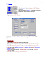
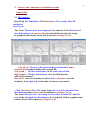
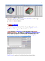
Example of 2D EB dose distributions in two-sided irradiated wedge with
film.
Curve 1 – EB dose distribution in the center line of film (in direction of
EB scanning) calculated with MC method.
Curve 2 – EB dose distribution in the center of a wedge material
calculated with Analitical method.
Curve 3 – EB dose distribution near the film boundary with wedge material
calculated with MC method.
You can “Delete selected curves” and make for all curves
“Normalization”.
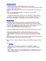
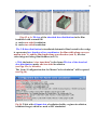
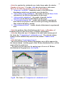
• The function of button "Compare" (right down side in the "Comparison
of calculated curves " frame) allows to make comparison of 2D dose
distributions for 2 any curves to obtain the values of differential and
integral deviations in % between compared curves. (see Fig. 20).
• For that, select the numbers of 2 compared curves and click the button
"Compare ".
• To copy the results comparison into your document, Click the button “Plot
mode 2D/3D”, if it is necessary, and then Click the button "Plot to clipboard"
and paste them to your document.
8. Dosimetry module
Block “Dosimetry” is intended for processing of dosimetric films with
experimental data and for preparing data for “Comparison” module.
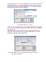
• Click the button “Dosimetry” in the Main form of the Software
ModeRTL (See Fig.1). The form of “Preparing of experimental
dosimetric data” will be opened for analysis of calculated and experimental
data of 2D absorbed dose distributions in an irradiated target
(See Fig.21.a).
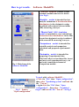
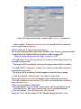
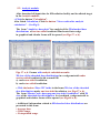
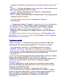
• Load a text file with experimental data from hard disk. A file may contains
three or two columns (X and Y, or X, Y1, Y2). (See Fig.21 b).
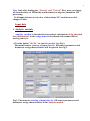
Loaded data are showing into the plot and into a grid and the buttons Move
and Invert, Cut and Scale, Convert data for Comparison appear.
(See Fig.22 a, b).
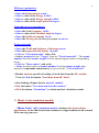
• To move selected curve to left or invert one you need to use the control
panel that will open when the button Move and Invert is pressed. To save
changes, press the button Apply.
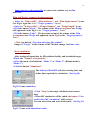
• Click the button Cut and Scale, to cut and scale curves data.
• To cut a part of curves, select by a tick the Marker 1 and move a mouse
pointer to the plot. In this point a vertical red line appears into plot. You
move it and place by left mouse clicking. It is a first limited line.
You make the same with Marker 2 and place a second red line.
(See Fig.22. a).