1
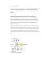
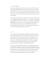
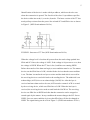
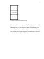
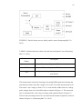
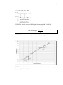
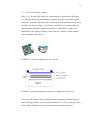
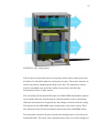
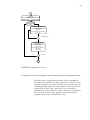
Design, construction and programming of an
air quality measurement device
LAHTI UNIVERSITY OF APPLIED
SCIENCES
Faculty of Technology
Degree Programme in Information
Technology
Software engineering
Bachelor’s Thesis
2014
Miikka Juomoja
Lahti University of Applied Sciences
Degree Programme in Information Technology
JUOMOJA, MIIKKA:
Design, construction and programming of
an air quality measurement device
Bachelor’s Thesis in Software Engineering, 45 pages
Spring 2014
ABSTRACT
The objective of this thesis was to design and build a prototype air quality
measurement device and to create a web application to support it. The main focus
in this thesis was to design and building the prototype. Another objective was to
test the compatibility of the given sensors and to determine if they are accurate
enough. The thesis was done for Aarhus University and it is meant to be a tool in
the university’s research projects.
The air quality measurement device measures temperature, humidity, particles,
carbon dioxide and other toxic gasses from the surrounding air. The device is
controlled with a microcontroller. Measurement data is sent through a mobile
communication network into a web server from where the user can analyze
measurement data with a web application.
The prototype’s circuit boards were designed and built from the scratch. The
circuit boards are manufactured by the client. The electronical sensors,
microcontroller and casing were chosen by the client before the project started.
The microcontroller was programmed with the C programming language.
The objectives were met: the prototype was built and it works as expected. Air
measurement sensors were compatible, although the measurement of the sensors
affected measurement data from other sensors. The problem was solved by
relocating the sensors. The prototype’s measurement data was accurate enough,
although calibration was not accomplished. The lifespan and replaceability of
measurement sensors were taken into account.
Key words: microcontroller, prototype, air quality, weather technology
Lahden ammattikorkeakoulu
Tietotekniikan koulutusohjelma
JUOMOJA, MIIKKA:
Ilmanlaadunmittausjärjestelmän
suunnittelu, rakentaminen ja ohjelmointi
Ohjelmistotekniikan opinnäytetyö, 45 sivua
Kevät 2014
TIIVISTELMÄ
Tämän opinnäytetyön tavoitteena oli suunnitella ja toteuttaa prototyyppi
ilmanlaadunmittausjärjestelmästä sekä siihen liittyvästä web-toteutuksesta. Työssä
keskitytään prototyyppiin, erityisesti suunnitteluun ja toteutukseen. Tavoitteena
on kartoittaa käytettävien ilmanlaatusensoreiden yhteensopivuusongelmat sekä
niiden tarkkuus. Tämä opinnäytetyö on tehty Aarhusin yliopistolle ja on
tarkoitettu työkaluksi yliopiston tutkimusprojekteja varten.
Ilmanlaadunmittausjärjestelmä mittaa ympäröivästä ilmasta lämpötilaa,
ilmankosteutta, pölyä, hiilidioksidia sekä muita haitallisia kaasuja. Laitetta
ohjataan mikrokontrollerilla ja mittaustulokset lähetään puhelinverkon välityksellä
palvelimelle, josta käyttäjä voi tutkia mittaustuloksia web-sivujen kautta.
Prototyypin piirilevy on suunniteltu ja rakennettu itse. Piirilevy on valmistettu
asiakkaan toimesta. Elektroniset sensorit, ohjainpiirit ja kotelo on valittu
asiakkaan toimesta ennen projektin alkua. Mikropiiri on ohjelmoitu Cohjelmointikielellä.
Työn tavoitteet saavutettiin; prototyyppi saatiin rakennettua ja järjestelmä toimii
oletetusti. Projektissa käytetyt ilmanlaatusensorit olivat yhteensopivia, vaikkakin
sensoreiden mittaustapa vaikutti muiden sensoreiden mittaustuloksiin. Ongelma
pystyttiin kiertämään sijoittamalla sensorit eri tavalla kuin alun perin oli
suunniteltu. Prototyypin mittaama tieto oli tarpeeksi tarkkaa vaikka kalibrointia ei
suoritettu. Suunnittelussa otettiin huomioon osien käyttöikä sekä niiden
vaihdettavuus.
Asiasanat: mikro-ohjaimet, prototyypit, ilmanlaatu, ilmastoteknologia
TABLE OF CONTENTS
1
INTRODUCTION
1
2
PROJECT GOAL
3
2.1
Used technologies
4
2.1.1
I2C
4
2.1.2
RS-232 and UART
6
3
4
5
6
7
CONTROLS AND SENSORS
8
3.1
MBED LPC1768 microcontroller
8
3.2
GSM/GPRS module
9
3.3
Anemometer
10
3.4
Temperature and humidity sensor
11
3.5
CO2 sensor
13
3.6
Particle sensor
14
3.7
CO, NO, NO2 and O3 sensors
18
HARDWARE DESIGN AND MANUFACTURING
21
4.1
MBED PCB
22
4.2
Sensor PCB
23
4.3
Casing and airflow
26
PROGRAMMING
29
5.1
Structure of the code
29
5.2
Sensor functions
31
5.2.1
Humidity and temperature functions
31
5.2.2
CO2 function
33
5.2.3
NO2, NO, O3, CO and anemometer functions
35
5.2.4
Particle sensor function
35
5.2.5
Connection through internet
37
5.3
Web application
39
TESTING
41
6.1
41
Final testing results
CONCLUSION
SOURCES
43
44
GLOSSARY
Anemometer = Wind speed sensor
Asynchronous communication = transmission of data without external clock
signal
AT Command = A set of commands to control Sim900 GPRS shield
C = Low level programming language
CO = Carbon monoxide, molecule
CO2 = Carbon dioxide, molecule
EAGLE = Cadsoft Eagle, PCB design software
GPRS = General Packet Radio Service
LED = Light emitting diode, electronic component
MBED = MBED LPC1728 microcontroller
NO = Nitric monoxide, molecule
NO2 = Natrium dioxide, molecule
O3 = Ozone, molecule
PCB = Printed Circuit Board
PPB = Parts per billion, air quality measure
PPM = Part per million, air quality measure
QSORT = Quick Sort Algorithm to sort data, C
STD = C standard function library
UART = Universal Asynchronous Receiver/Transmitter
USB = Universal Serial Bus
1
INTRODUCTION
The client of this batchelor’s thesis is Aarhus University, Herning. The
researchers want to know how well the Danish THOR modeling system applies in
campus and nearby areas:
Since 1996, the National Environmental Research Institute
(NERI), Denmark, has developed a comprehensive and unique
integrated air pollution model system, THOR. The model system
includes several meteorological and air pollution models
capable of operating for different applications and different
scales. The system is capable of accurate and high resolutions
three-days forecasting of weather and air pollution from
regional scale over urban background scale and down to
individual street canyons in cities. (Brandt 2012.)
The air quality may be influenced by a power plant located nearby, and some
concerns have been shown about the pollution which is comes from neighbor
countries with the wind. Professional accurate air quality sensors are expensive
and the nearest professional sensors are located 32 kilometers from the university.
The easiest solution is to create a small and cheap device which gives fairly
accurate measurement values. This device will be a tool to determinate if the
modeling system is working as it should. Also it will be used to determinate
University’s indoor air quality.
The objective was to create a prototype of an air quality measurement device with
the help of another exchange student. The project included a server which handles
the incoming data and a website which helps researchers in analyzing the data.
The device should measure air molecules, particles, humidity, temperature and
wind speed. Every hour data is sent into the server, from where the researchers
can receive the data as files or in linegraphic format and examine it. The main
focus is to study and test the compability, measurement accuracy and lifespan of
the sensors. This thesis addresses with only the design and production of the
prototype.
The first research problem was to create a prototype device from prechosen
sensors, microcontroller and casing. The main task was to create two printed
2
circuit boards (PCB) to control all the sensors and the mobile networking
microchip. The second research problem was collecting the data from the devices
which can be located anywhere in the campus area or nearby locations like
Herning city. The device sends data once an hour, and there has to be a server
which manages the data. The researchers can collect data into a website from
where it can be retrieved. The third research problem was the airflow and sensor
compability. How the airflow affects the sensors, and whether the other sensors
affect the measurements?
In the first section of this thesis, you are presented with the sensors used in this
project. All the theoretical background of sensors is explained. The manufacturers
have provided information in datasheets and in accurate explanations the
functionality of the sensors. The manufacturer’s datasheets are the main source of
information for this thesis. The thesis continues into circuit board design and
explaining device code structure and solutions and finally reveals the test results
and outcome.
3
2
PROJECT GOAL
The client of the project was Aarhus University. Before the project began they had
chosen and purchased all measurement sensors, MBED microcontroller and
prototype’s casing. They provided all necessary instruments, server space and
software.
The main goal was to create an air quality control device prototype, a PHP server
script and a webclient for the user. The project was built over repository
architecture. In repository architecture, devices communicate through a shared
data server and in this project air quality control devices (later referred as the
prototype) only send data into the web server. The users read the measured data
from the repository via the webclient. Figure 1 shows all entities and their
relations in this project.
The prototype was only one part of the project. The measurement data must be
stored into a unified data storage, from where it can be rerieved. The second part
of the project was to develop a PHP server script which handles data storing and
retrieving with MySQL database queries. The third part of the project was to
create the webclient, which generates tables and graphs from the sensor data to the
user.
FIGURE 1. Project topography.
4
2.1
Used technologies
The prototype’s building process can be split into two parts. The first part is the
designing and manufacturing of the device. The design of the device’s printed
circuit boards (PCB) was done with Cadsoft Eagle PCB design software. Cadsoft
Eagle is one of the most used PCB design software in the market. The project was
done with a freeware version of the software, which limited the maximum size of
the PCB board.
The second part of the project was programming. The prototype was programmed
with C programming language using Google’s C++ styling guide. The only library
needed is MBED microcontroller’s own software development kit (MBED-SDK).
MBED-SDK is an open source C/C++ library, which gives the programmer lowlevel and high-level tools to control their own MBED microcontroller, for
example an inter-intergrated circuit (I2C) or serial connection controls, which are
also used in this project. (NXP Semiconductor 2012b.)
2.1.1
I2C
I ²C is a databus originally manufactured by Philips Semiconductor (nowadays
known as NXP Semiconductor). I2C is designed to be a bidirectional 2-wire bus.
The communication is 8-bit oriented and it can make up to 100 kbit/s in the
standard mode, up to 400 kbit/s in the Fast-mode, up to 1 Mbit/s in Fast-mode
plus, or up to 3.4 Mbit/s in the High-speed mode. The databus has high noise
immunity, wide operating temperature and supply voltage range, and it has
extremely low current consumption. (NXP Semiconductor 2012a.)
One or more devices (usually microcontrollers) are working as a master device.
One I2C bus has a maximum of 128 devices because of the address range, which
is the byte’s last seven bits. The master can communicate with one slave device at
a time and its duty is to start data transfer, generate clock signal and to end data
transfer. All devices are connected by the same two wires: Serial Clock Line
(SCL) sends the clock signal and Serial Data Line (SDA) sends data.
5
Identification of the device is made with byte address, which needs to be sent
when the connection is opened. The first bit of the slave’s byte address specifies
the device either into read (1) or write (0) mode. The latest version of the I2C bus
needs pull-up resistors from the power line to both SCL and SDA wires as shown
in Figure 2. (NXP Semiconductor 2012a.)
FIGURE 2. Structure of I2C line (NXP Semiconductor 2012a).
When the voltage level is less than 80 percent from the total voltage pushed into
SDA and SCL lines, the voltage is LOW. If the voltage is 80 percent or over, then
the voltage is HIGH. When the I2C bus is free, both lines are running HIGH.
Before the transfer of the data can begin, a start condition must be set. The master
device sets the SDA line to LOW, which tells the devices that the start condition
is set. The data is transferred one byte at a time and the ninth tick is reserved for
the receiving device to send a bit back to the sending device. The ninth tick is an
acknowledge (ACK) bit or a no-acknowledge (NACK) bit. After the byte is
received and more data needs to be sent, ACK must be returned. ACK is created
by the receiving device, which sets SDA line to LOW. When the last byte is
received, the receiving device needs to send back the NACK bit. The receiving
device sets SDA line to HIGH and after that the connection can be stopped or
started again by the master. In stop condition the master changes the SCL line to
HIGH, if no new start condition is given, then SDA line will also be changed to
HIGH. The signal timing can be seen in Figure 3. (NXP Semiconductor 2012a.)
6
FIGURE 3. I2C timing chart (NXP Semiconductor 2012a).
2.1.2
RS-232 and UART
RS-232 is a full duplex serial communication standard, which allows
communication in both directions. The maximum line length should be kept
relatively short, because a longer cable would have alternating voltages on each
side of the ends, which would increase noise margin of the signal. Noise mostly
affects the data signal and might corrupt the transferred data. (Campbell 1989,
50.)
The simplest RS-232 needs only two data transmission lines, the transmit
exchange data (TxD) and the received exchange data (RxD), and a common
ground line. TxD pin sends data into the receiving device’s RxD pin. When the
voltage is between three and 15 volts, the line logic is set to zero (Space), and
when the voltage is between minus three and -15, the line logic is set to one
(Mark). The area between minus three and plus three volts is called the transition
region where the line does not know which logic level it is on. The logic levels
can be seen in Figure 4. When the line is free, it is set to logic level zero.
(Campbell 1989, 50.)
7
FIGURE 4. Logical levels (Campbell 1989, 49).
Universal asynchronous receiver/transmitter (UART) is a piece of hardware which
is used in serial communication. When sending, UART splits a byte into
individual bits and forms a bit transmission by adding a start bit and one or two
stop bits before sending the message through the communication lines. While
receiving, UART saves the data bits into a buffer and resamples the bits back into
bytes. When the buffer overloads, it discards the incoming data bits or replaces the
old data bits with the new. (Campbell 1989, 25.)
8
3
3.1
CONTROLS AND SENSORS
MBED LPC1768 microcontroller
MBED LPC 1768 was chosen to be the microcontroller of the prototype. The
main reasons for this were the amount of serial and I2C ports and the
manufacturer’s high level C/C++ API. The manufacturer is NXP Semiconductor,
which is the same company that owns the rights to I2C bus. The microcontroller is
based on a 32-bit ARM® Cortex™-M3 design. The microcontroller includes a
built-in USB programming interface, which is as simple as using a USB Flash
Drive. (NXP Semiconductor 2014b.)
The core is running at 96MHz and the microcontroller has 32KB of RAM
memory and 512KB of programmable FLASH memory. The microcontroller’s 40
pins consist of 26 digital input and output pins, three serial ports, two I2C ports
and other I/O interfaces as shown in Figure 5. The Microcontroller works within
the limits of 4.5 to 9 volts and it can give 3.3 or 5 volts out. The built-in USB
programming interface works by dragging and dropping files from the computer.
An online compiler is included with purchase of the microcontroller. (NXP
Semiconductor 2014b.)
FIGURE 5. MBED LPC1768 microcontroller’s design and features (NXP
Semiconductor 2014b).
9
3.2
GSM/GPRS module
The GMS/GPRS shield is manufactured by an open hardware facilitation studio
ElecFreaks. The shield uses a SIM900 GPRS/GSM module, manufactured by
SIMCom Wireless Solutions Co., Ltd. The SIM900 module is working with five
volts and it has low power consumption of 1.5mA in the sleep mode. The module
is using a quad-band engine, which means that the module is compatible with four
main-GSM frequencies. The module stores SMS messages and phonebook data
into a SIM card. There is a built-in implementation of the Internet protocol suite
(TCP/IP) networking model. The communication is done with serial
communication and it has a maximum buffer size of 556 bytes. The module
supports an antenna and an audio interface, which can be seen in Figure 6.
(ElecFreaks 2014.)
The SIM900 module is controlled via AT commands (based on GSM 07.07, 07.05
and EFCOM enchanced AT commands). The AT commands originate from a
Hayes command set and they are pre-programmed inside the SIM900 by the
manufacturer. The AT Commands are series of short text strings which combined
together forms commands for operations such as changing parameters,
establishing connection into internet or sending an SMS message. The commands
are created to ease the use of the microchip. (Shanghai SIMCom Wireless
Solutions 2009.)
10
FIGURE 6. GSM/GPRS module (ElecFreaks 2014).
3.3
Anemometer
Anemometer (Figure 7) is manufactured by Chinese Shaanxi Enjoy Imp & Exp
Co., Ltd. The sensor does not need any external power because the voltage is
formed by the rotation of the sensor. The direction of the rotation affects the
output of the sensor: if the sensor rotates backwards, then the voltage will be
negative.
The output voltage corresponds to the wind level (wind speed) as shown in Figure
8. The sensor outputs a maximum of five volts where one meter per second is
equal to 0.4 volts. MBED can read only the maximum of 3.3 volts so this sensor
can measure up to 8.25 meters per second. The sensor must be placed in an open
space where the wind comes straight into the sensor. The measurement value is
lower if wind is obstructed from any angle. The sensor does not require any
calibration.
11
FIGURE 7. Anemometer.
FIGURE 8. Graph for the relationship between the output voltage and wind level.
3.4
Temperature and humidity sensor
Temperature and humidity values are measured from one sensor, Honeywell
HumidIcon digital humidity/temperature sensor (HIH6130, Figure 9). The sensor
is operating with 3.3 volts, and in the sleep mode it only requires one
12
microampere of power. It can be controlled either with SPI or I2C buses. The
sensor works in the range of 5 to 50 degrees of Celsius and from 10 to 90 percent
of relative humidity (%RH). The true accuracy level of humidity and temperature
can be seen in Table 1. The accuracy of the humidity changes at the maximum of
±1.2 %RH in five years. The accuracy of the temperature changes at ±0.05
degrees of Celsius per year in five years. (Honeywell International 2013.)
FIGURE 9. Humidity and temperature sensor (SparkFun Electronics 2014).
TABLE 1. Total error band of temperature/humidity sensor (Honeywell
International 2013).
13
The sensor uses a laser trimmed, thermoset polymer capacitive sensing element,
which provides resistance to most application hazards such as condensation, dust,
dirt, oil, and common environmental chemicals. The polymer helps to provide
stability and reliability, and it works well in indoor and outdoor environments.
Every sensor goes through a 12-hour rehydration process at 75 %RH and a fivehour rehydration process in conditions of 50 %RH, to correct the temperature
offset. This process provides long term stability and removes the need of
recalibration of the sensor. (Honeywell International 2013.)
3.5
CO2 sensor
The CO2 sensor is called K-30 (Figure 10) and it is manufactured by CO2Meter
Inc. The Sensor measures CO2 values with infrared light. CO2 absorbs the infrared
light and the sensor measures the amount of light which is passes through the gas.
The sensor is works with five volts and it communicates either through I2C or
serial communication. The maximum measurement range is 10 000 ppm of CO2,
it needs one minute to warm up, it stabilizes itself after the first hour. (CO2Meter
Inc. 2014.)
FIGURE 10. CO2 sensor (CO2Meter Inc. 2014).
The sensor includes a built-in self-correcting algorithm, which tracks the lowest
reading for the last seven days and corrects it comparing to an expected fresh air
14
value of zero or 400 ppm of CO2. The calibration is useful when the sensor is used
outdoors. The tuning speed is limited for 30 ppm per week by the manufacturer.
The automatic calibration can be added by adding a jumper wire in Din1 (400
ppm) or Din2 (0 ppm) as shown in Figure 11. Indoors, the calibration must be
disabled. (CO2Meter Inc. 2014.)
FIGURE 11. Schematics of CO2 Sensor (CO2Meter Inc. 2014).
3.6
Particle sensor
The particle sensor module is called DSM 501 (Figure 12) and it is manufactured
by Samyoung S&C Co., Ltd. The sensor is designed for rooms or casings smaller
than 30m3 to measure particles bigger than one micrometer. The sensor is a costefficient solution to measure a quantity of floating particles which can cause
15
allergy or respiratory disease. The sensor doesn’t need calibration and it is
accurate after one minute from the startup. The sensor must undergo maintenance
every six months: lens must be wiped clean to prevent measurement errors.
(Samyoung S&C Co. 2012.)
FIGURE 12. Particle sensor (Samyoung S&C Co. 2012).
The particle sensor uses a resistor to heat air for 30 seconds. The heat creates an
updraft, which draws outside air into the sensor while a light emiditing diode
(LED) blinks. A built-in detector measures particles from the amount of light
passing through the air. The detector sends data about the amount of particles
through an amplifier circuit into two output circuits as shown in Figure 13. Output
circuit two is factory calibrated and always gives a pulse-width modulation
(PWM) output from all particles which are over one micrometer. Output circuit
one’s PWM signal can be selected. This pin can send the amount of particles
which are bigger than 2.5 or 1.75 micrometer. The measurement size is controlled
with a resistor between control and ground pins. Table 2 shows the relation
between the resistor size and measured particle size. (Samyoung S&C Co. 2012.)
16
FIGURE 13. Particle detect process inside particle sensor (Samyoung S&C Co.
2012).
TABLE 2. Relation between resistor size and measured particle size (Samyoung
S&C Co. 2012).
Resistor value
(Ohms)
Description
Open (no resistor)
Preset sensitivity (over 2.5 micrometer)
100K
Half sensitivity (over 1.75 micrometer)
27K
Equal sensitivity of Output circuit two (over one
micrometer)
The measurement is done by listening to incoming PWM signal and counting the
total amount of time when the voltage is low in the 30-second measurement cycle.
The sensor’s low voltage is from 0.7 to 1.0 volts and the width of the low voltage
pulse changes from 10 to 90 milliseconds, as shown in Figure 14. The measured
time is translated into a low ratio percentage with equation shown in Figure 15.
The low time percentage has to be converted into the amount of particles, which is
shown in Figure 16. (Samyoung S&C Co. 2012.)
17
FIGURE 14. Particle sensor’s PWM signal (Samyoung S&C Co. 2012).
FIGURE 15. Low time percentage calculation (Samyoung S&C Co. 2012).
10
9,2
9
8
8,0
Low Ratio [%]
7
6,8
6
5,6
5
4
4,0
3
2,4
2
1
0,8
0
0
0,2
0,4
0,6
0,8
1
1,2
1,4
1,6
Particle [mg/m3]
FIGURE 16. Relation between the amount of particles and low ratio percentage
(Samyoung S&C Co. 2012).
18
3.7
CO, NO, NO2 and O3 sensors
The CO, O3, NO and NO2 sensors are manufactured by Alphasense Ltd (Figure
17). All four sensors are electrochemical and they have three electrodes in them,
which are connected to the three pins coming out from the porcelain casing. These
electrodes are shown in Figure 18. All three electrodes are in contact with each
other through hydrophilic separators (labeled as wetting filters in Figure 18),
which allows the capillary transport of the electrolyte, which is usually sulfuric
acid. (Alphasense Ltd. 2012 c.)
FIGURE 17. NO sensor (Alphasense Ltd. 2012 d).
FIGURE 18. Schematic diagram of the sensors (Alphasense Ltd. 2012 c).
Gas comes into contact with a working electrode through a gas diffusion barrier.
In the working electrode, electrochemical oxidation (CO, NO) or reduction (NO2)
occurs. The working electrode is directly exposed to all gases in the air.
19
Therefore, the electrode may absorb wrong gases from the air and become
poisoned, which breaks the sensor. The sensor might be recovered if it is infused
with other gases like sulfur to reverse the poisoning. (Alphasense Ltd. 2012 c.)
Alphasense Ltd (2012) describes the functioning of the counter electrode in this
way: “The counter electrode balances the reaction of the working electrode – if
the working electrode oxidises the gas, then the counter electrode must reduce
some other molecule to generate an equivalent current, in the opposite sense.” The
counter electrode must keep up with the working electrode. The amount of current
is equal to the amount of reactions balanced by the counter electrode. The most
common reaction is the reduction of oxyden, if the counter electrode cannot get
enough of oxygen, then the whole sensor stops sending valid data until there is
enough oxygen again. (Alphasense Ltd. 2012 c.)
The reference electrode ensures that the working electrode is always in the correct
region of the current voltage curve. This affects the constant sensitivity, linearity
and the minimum sensitivity of the sensors to interfering gases. There is also a
stabilation time until sensors start to send valid data. These times are shown in
Table 3. Because of the way that the sensors work, their lifespan is short. They
need to be replaced after the original signal drops under 50 percent. The
measurement accuracy also deteriorates over time. Deteriorating and lifespan
information is shown in Table 4. (Alphasense Ltd. 2012 c.)
TABLE 3. Stabilation time of Alphasense sensors (Alphasense Ltd. 2012 b).
New sensor or after long
After brief removal e.g.
period of removal
for replacement
(Hours)
(Minutes)
CO
2
10
NO
12
12 Hours
NO2
2
10
O3
2
10
Sensor
20
TABLE 4. Deteriorating and lifespan of the Alphasense sensors (Alphasense Ltd.
2012 b).
ppb change in year
months until 50% of the
(lab environments)
original signal
CO
±100
36
NO
0 - 50
24
NO2
0 - 20
18
O3
0 – 50
18
Sensor
21
4
HARDWARE DESIGN AND MANUFACTURING
The prototype was designed with a freeware version of Eagle. The freeware
version limits the useable board size into 100 x 80 mm. One board was too small
to hold all electronic components so design was changed from one PCB to two
PCBs. The first board has only a MBED microcontroller, screw terminals and
powerjacks. The second board contains all measurement sensors except the CO2
sensor and the anemometer. The anemometer was placed outside the casing with
screws and its wires are connected into the sensor PCB. The overall design can be
seen in Figure 19. Sensors were not soldered straight into the board. Headers are
soldered into the PCB’s, and sensors are attached to them so the sensors and
microcontroller can be removed or replaced easily. The device gets its power from
two power adapters, which are connected to the electrical grid.
The CO2 sensor and the GSM/GPRS shield already had existing PCB layouts so
they are not built into the MBED or the sensor PCBs. Two small PCBs were
needed, to enable connection between the CO2 sensor and the GSM/GPRS shield
with MBED PCB. These two PCBs hold headers for the sensor pins, the headers
lead into screw terminals from where they are connected into the two main PCBs.
This way the CO2 sensor and GSM/GPRS shield are repleacable and both are
connected into MBED PCB with wires. The anemometer is connected into the
Sensor PCB’s screw terminals.
22
FIGURE 19. Prototypes overall design.
4.1
MBED PCB
The MBED board is simple. It holds a MBED microcontroller, 24 screw terminals
and two powerjacks. The communications between PCBs are done with screw
terminals and wires.
The powerjacks are connected with five and six-volt adapters. Five-volt
powerjack is connected with a screw terminal where the line continues into the
GSM/GPRS shield, the CO2 sensor and the sensor PCB. Six-volt powerjack is
connected with the MBED voltage input to provide power to the MBED. The line
continues into the sensor board through screw terminals. The third voltage comes
out from the MBED: a 3.3-volt line is connected with the sensor PCB through
screw terminals. One side of the PCB is a ground plate, covered with copper. All
ground pins are connected to this copper layer.
23
The MBED is connected to the board through a 40-pin header so it can be
replaced easily. Most of the MBED pins are connected into a screw terminal from
where they continue into corresponding sensors or into the sensor PCB. All pins
are not needed and they are not connected. The main purpose was to add pins,
which would also be useful in the future. All I2C and serial ports, analog inputs
and a few digital outputs are connected. In addition, the pulse-width modulation
output pins are connected, because they can control fans or work as digital
outputs. The PCB design can be seen in Figure 20.
FIGURE 20. MBED PCB.
4.2
Sensor PCB
There are three different voltage inputs coming from the MBED PCB, five-volt
for the particle sensor, six-volt for the Alphasense sensors and 3.3-volt for the
humidity and temperature sensor. The backside of the sensor PCB works as a
ground layer similar to the MBED PCB. The sensor PCB holds all the
measurement sensors except the CO2 sensor. The board size limitations of Eagle
forces the Alphasense sensors to be placed on the edge of the board. All sensor
pins are attached to screw terminals. The design is seen in Figure 21. There are
also two screw terminals reserved for the anemometer which is attached outside
the casing.
24
FIGURE 21. Sensor PCB design.
Figure 22 shows the electric design of the humidity and temperature sensor. The
SDA and SCL lines are powered from the same power source as the humidity and
temperature sensor. Two 3.3kΩ pull-up resistors are connected between the SDA
and SCL lines and the power source. The alarm output high (AL_H) and alarm
output low (AL_L) pins are not connected because they are not used.
FIGURE 22. Humidity and temperature sensor design.
25
Figure 23 shows how the circuit boards of the Alphasense sensors are built. All
four sensors were pre-assembled into circuit boards by the manufacturer. The
Alphasense PCBs have six pins where three are ground pins. The voltage input
(six volts) is common and the measurement signal (measurement value) comes
from the IC1 pin (Vout1). The IC2 pin (Vout2) is reserved for calibration and
normally it will not be needed. When the sensor is old enough, it will be replaced.
FIGURE 23. Alphasense sensor design (Alphasense Ltd. 2012 a).
The biggest problem with the design was the placement of the humidity and
temperature sensor. The sensor is placed next to the particle sensor, and when it is
measuring, it heats the air next to it and the heated air affects the humidity and
temperature sensor values. The Alphasense sensors measure air quality by burning
reaction and they also affect the humidity and temperature sensor. A simple fix for
this is presented in Chapter 4.3. There is also a problem with the anemometer. A
26
negative voltage breaks up the MBED microcontroller and it must be changed into
apositive voltage with an operational amplifier.
4.3
Casing and airflow
A plastic casing was provided at the beginning of the project. It needed to work
only as testing environment before the final layout was confirmed. The original
idea was to assemble all sensors inside, drill holes on two sides of the casing and
let air flow naturally. The sensors were assembled into the casing, and a set of
problems were noticed.
The particle sensor heats the air for half of the one-minute measurement cycle and
the Alphasense sensors use burning reaction to measure toxic gasses. The air is
not changing inside the casing. When the casing’s cover was closed, the CO2
values rose slowly and the temperature and the humidity values were different
from the values measured outside the casing. The device needs airflow and this
problem can be solved by creating an underpreasure with fans. The airflow affects
the measurement of the Alphasense and the particle sensors and it must be
considered in the design. The solution for the casing problem is to split the device
into two sections. The new casing layout is presented in Figure 24.
27
FIGURE 24. New casing layout.
The first part (I) has all the sensors (except the particle sensor) coming out from
the holes of a wall which splits the casing into two parts. The sensors measure air,
which is just barely changing by the help of two fans. The Alphasense sensors
must be assembled to the end of the airflow because they will affect the
measurement values of other sensors.
The second part (II) has both PCB boards, the GSM/GPRS shield and the particle
sensor. Both of the fans stop blowing air when the particle sensor is measuring.
When the measurement is completed, the fans change air slowly from the casing.
The antenna of the GSM/GPRS sensor should come out from the casing. There
also should be a hole for the two buttons which control the GSM/GPRS shield.
The anemometer needs to be placed outside the casing because it is too big to be
assembled inside. The sensor can be attached easily to the cover with a magnet or
28
screws. The cord of the sensor is attached to sensor PCB’s screw terminal and it
needs a small hole on the side of the casing. Figure 21 shows that the screw
terminals of anemometer are located on the opposite side of PCB’s other screw
terminals. The reason for this layout is the length of the anemometers’s cord,
which is only ten centimeters long. This is not a problem in the final device
because the casing will be smaller.
The last thing which needs to be considered is the attaching of the board. The
boards can be located in places where normal people cannot reach, and the
persons attaching the boards might not be familiar with the technology. There has
to be one or two LEDs attached into the casing. The LEDs inform startup errors to
the attacher. If the errors are not solved automatically by the program, then a spare
device must be attached and the malfunctioning device must be returned to the
maintenance department. Mostly these errors will occur with the GSM/GPRS
shield and they usually consist of a bad connection or a simcard malfunctioning.
29
5
5.1
PROGRAMMING
Structure of the code
In the beginning of the program, the device generates arrays for every
measurement value and three test calibration values for CO, NO and NO2. There
are a total of 13 arrays. Once a minute the program runs all the measurement
functions and saves the returned measurement data into a corresponding array.
The main loop runs once an hour. One loop runs through all sensor functions 59
times and sorts all arrays from the lowest value to the highest using the Qsort
function of the C standard library. After the sorting, the program sends median
values (29th value) to the server. The median values are used because
occasionally there will be incorrect measurement values. The measurement values
can differ from the normal measurements, and those error values should be
filtered from the true data.
In the background, a timer object is measuring how long it takes to run all the
functions in microseconds. The timer value is reduced from one minute and the
outcome is the value which the program needs to wait until the next loop can start.
The sensor functions are never coherent and this way the sensor loop of the
application runs exactly one minute. The last loop runs for two minutes, and in
that time window, the last data is retrieved, data is sorted and sent into the web
server. The structure of C code is presented in Figure 25.
30
Power on
Create 13 Arrays
Establishe connection to the web server
Start hour loop
Infinite
Start minute loop
Wait X Microseconds
Start Timer
Run all 13 Measurement functions
Stop Timer
No
59th Minute Loop?
Yes
End minute loop
Start Timer
QSort 13 Arrays
Send data into the web server
Stop Timer
End Hour Loop
Yes
Power on?
No
FIGURE 25. Structure of C code.
To add more speed to the program, some functions are done by doing them inline.
Inline function is a small function whose code is expanded in
line rather than called. Every time a function is called, a series
of instructions must be executed, both to set up the function call,
including pushing arguments onto the stack, and to return from
the function. In some cases, many CPU cycles are used to
perform these actions. However, when a function is expanded in
line, no such overhead exists, and the overall speed of your
program will increase. (Schildt 2003, 264)
31
5.2
5.2.1
Sensor functions
Humidity and temperature functions
The temperature and humidity sensor is connected through an I2C bus. The device
returns four bytes of data, which contains both humidity and temperature. The
process can be seen in Figure 26. After receiving both values, they must be
converted into float values and calculated through equations provided by the
manufacturer. These calculations are presented in Figure 27 for humidity and
Figure 28 for temperature. (Honeywell International 2011.)
FIGURE 26. Humidity and temperature data communication through I2C
(Honeywell International 2011).
FIGURE 27. Equation for the percentage of relative humidity (Honeywell
International 2011).
FIGURE 28. Equation for temperature (Honeywell International 2011).
32
The humidity and temperature measurement values are read from the same sensor.
The master device (MBED) needs to wake up its slave device (humidity and
temperature sensor) so the device understands that the MBED is listening to the
I2C line and the humidity and temperature sensor can start to send measurement
values. This waking up process is done by starting the I2C line and sending one
byte to the line. The byte’s first seven bits contain the slave’s address (0x27) and
the last bit will be a write bit (0), which tells the slave to be on writing mode.
Lastly, the I2C line needs to be closed.
When the sensor is woken, the program requests humidity and temperature
readings. This is done by opening the I2C line and sending the address byte again.
This time the first seven bits are the address of the slave but the last bit needs to
be changed into the read bit (1). This is done by changing the address with a
bitwise OR operator. After the request is sent, the MBED starts to listen. There are
a total of four bytes to receive. The first two bytes are the humidity value’s high
and low bytes which must be acknowledged with an acknowledge bit (1). The
third byte sent by the slave is the temperature value’s high byte which also needs
to be acknowledged. The last byte is the temperature value’s low byte which must
be no acknowledged by sending a zero bit and closing the I2C line. This whole
process can be seen in Figure 29. The bytes are loaded directly into unsigned char
values, and acknowledgements are handled with MBED SDK’s read functions
parameters.
FIGURE 29. Reading data using I2C.
The received four bytes need to be edited that they will present the correct 14-bit
data. The two highest bits of the humidity’s high byte are command bits, and
33
those bits are not part of the calculation. They need to be changed into zero before
thehigh and low bytes are combined. This is done by using a bitwise operator
AND with the hexadecimal value 0x3F. The last two bits of the temperature’s low
byte are zeroes and those are not part of the calculation either. After combining
temperatures high and low bytes, the formed value is shifted to the right by two
bits, which corrects the value. The data is calculated and returned out from the
function by using pointer values given as formal parameters in the function call.
The data transfer and the assignment code can be seen in Figure 30. Calculation in
lines seven and eight are compressed calculations from Figures 27 and 28.
FIGURE 30. Changing humidity and temperature data into correct values.
5.2.2
CO2 function
The CO2 sensor uses a serial port to communicate with the MBED. At the
beginning of the function, a list of command bytes are sent into the sensor.
Command bytes inform the sensor which setup it has to use. The bytes are
explained in Table 5. After sending the command bytes, the program needs to wait
for 15 seconds for the sensor to measure the amount of CO2. The CO2 value
request can be seen in Figure 31.
34
TABLE 5. CO2 command bytes.
Serial Address
Command
I2C Address
How many
Checksum
(1 Byte)
(1 Byte)
(2 Bytes)
bytes to read
(2 Bytes)
(1 Byte)
0xFE
0x44*
0x00
0x08
0x02
*Command Bytes: 0x46 – EEPROM Read, 0x44 – RAM Read
Figure 31. Request CO2 value.
When the CO2 is measured, the program starts to read the data from the serial
buffer. The CO2 sensor returns a set of bytes where the fourth and fifth bytes are
the ones holding the measurement data. Other bytes are not needed in this project.
The high and the low bytes are combined and returned into the main loop.
Reading CO2 data is shown in Figure 32.
FIGURE 32. Read CO2 data from buffer.
35
5.2.3
NO2, NO, O3, CO and anemometer functions
The NO2, NO, O3, CO and wind speed values are received as analog inputs. The
analog inputs are pins that read the amount of voltage coming into the MBED
microcontroller. The MBED can only read voltages from 0.0 to 3.3 volts and the
value can be read from the pin with two different MBED-SDK’s built-in
functions. The normal read function changes the voltage difference into a float
value from zero to one. A more accurate way is to use function read_u16. This
function changes the voltage into an unsigned integer from zero to 65535. The
program uses a basic read function because it makes calculations more readable
and there is no need for accuracy that the read_u16 function provides.
The analog input works with one function call so all the sensor functions are small
and simple. The functions return voltage values, which need to be multiplied by
3.3 volts and to be calculated by correct calculations found in Chapters 3.3 and
calculations which Alphasense Ltd provided. These calculations can be seen in
Figure 33. The Alphasense sensor functions are compressed to increase the speed
of the program. This solution makes the calculations smaller, faster and more
readable. All the measurement functions are built as inline functions to increase
speed.
FIGURE 33. Inline functions.
5.2.4
Particle sensor function
The particle sensor is also connected through an analog input and it measures half
of the one-minute measurement cycle. The calculation of the voltage low time is
36
done with an interrupt class. Two timer classes are needed from the MBED-SDK,
one for measuring the total time and the second to measure the low time.
The interrupt class detects when a voltage is on a falling edge (line 14) and it
starts a function startTimer, which counts the amount of milliseconds of the
downtime. When interrupt is on the rising edge (line 15), class runs a pauseTimer
function which adds counted milliseconds into a total measurement variable
(tempSeconds) and resets the timer. The second timer (measurementTimer) runs
inside a while loop. The while loop does not do anything else but wait until 30
seconds has passed. 30 second is the time needed the sensor to measure the true
amount of particles in the air. Measuring process is show in the lines 1 – 19 in
Figure 34.
FIGURE 34. Calculation of particles from particle sensor.
The measured milliseconds are changed into a low ratio percentage and
calculated. This is shown in lines 21 to 25 of Figure 34. There are two different
calculations because the slope changes at the value of 5.6. In line 21, the amount
37
of seconds is changed into a low time percentage, and the amount of particles are
calculated in lines 23 and 25. The calculations are done from Figure 16 and they
are presented in Figures 35 and 36.
FIGURE 35. Calculation when low ratio percentage is equal or under 5.6.
FIGURE 36. Calcultion when low ratio percentage is over 5.6.
5.2.5
Connection through internet
The connection between the server and the devices is done through the SIM900
GSM/GPRS shield. The shield opens a connection to the server’s PHP script and
it is controlled with AT commands. The AT commands are passed as a printf
function through a serial connection.
When all settings are established, connection through HTTP protocol is
initialized. After establishing the start commands shown in Figure 37, the
connection is working until the GSM/GRPS shield is rebooted. After every
command, the GSM/GPRS shield generates return statements, which are read with
a getc function so the buffer does not overload. There are a set of commands
which block return statements, but they are not used because return statements are
needed in the final product to confirm that the connection is established.
38
FIGURE 37. Waking up GRPS module.
The communication is done with the AT+HTTPPARA and AT+HTTPACTION
commands. The first command needs the URL of the server with the measurement
data at the end of the URL. The data is sent using a HTTP GET request, so all
parameters are included in the URL. The GET request is used instead of a HTTP
POST request because the GET request makes thecode shorter, faster and
readable. There are two different cases where there is a need to send data. When
the device is powered, it informs the server that the device is online, and after
every hour the device sends measurement data. The AT+HTTPPARA command
fills the buffer and the AT+HTTPACTION sends the created request to the web
server. In Figure 38, the device’s ID is sent into the server, so the server knows
that the prototype is connected and will send measurement data every hour.
FIGURE 38. Sending data using HTTP GET request.
39
5.3
Web application
The prototype was only one part of the project. The data needs to be presented for
the user through a web application. The web server holds a small PHP script,
which receives data from the prototype and adds it into a MySQL database. The
web application requests measurement data from the PHP script and presents it for
the user.
The website is built from two sections. The first section includes a data table,
where the user can see accurate measurement data from each hour. This was done
by using DataTables javascript library. DataTables creates automatic table pages
from the HTML table data. DataTables add table pages, sorting and searching,
which makes the table versatile. The DataTables output can be seen in Figure 39.
The user needs to retreive data from the website, so they can reference to them
when needed. This is done by using TableTools which is a plugin for DataTables.
TableTools is an Adobe Flash element which is added above the search field in
Figure 39. This button toolbar allows the user to copy selected data into the
clipboard, print or download data as a PDF, XLSX or CVS file. DataTables and
TableTools are jQuery plugins.
FIGURE 39. Datatable in the website.
The second section of the website is a page which represents data as a graph. This
is done with Flot javascript library. Flot is a jQuery plugin which creates
40
automatic graphs from the given data. The graphs can be retrieved from the
webpage as pictures. Additional tools are added so the user does not need to create
graphs by hand. The additional tools are overview and zoom, which allows the
user to retrieve only small parts of the graph. Figure 40 shows the web solution
and zooming.
FIGURE 40. Website’s automatic graphs.
41
6
TESTING
Testing was done several times over the production time of the device. All the
values except temperature and humidity were compared with default air pollution
values from the European Environment Agency’s website. There were not any
existing sensors to test values except humidity and temperature, so both values
were tested with normal electronic household sensors.
At the beginning all sensors were assembled into a breadboard with MBED.
Sensors were programmed and they were tested for the first time. Measurement
values were compared to corresponding normal air pollution values. The next test
was conducted after all sensors were assembled into the PCB’s. The purpose of
this test was to try getting sensors to work all together and to give reasonable air
pollution values.
The last test was run after both PCB’s were assembled into the casing. This test
was the most important one because it showed what went wrong in the design and
if there was something affecting the test results. The main goal was to get the code
as ready as possible. Calibrations of the the three sensors were only a test. Other
calibrations were not done because the device was only a prototype. The device
was measured for a long period of time. Secondary focus was on MBED’s
memory control and the amount of data sent to the server. With this test the
amount of data sent through the GSM/GPRS shield was measured. The last test
took place in varied locations, indoors and outdoors.
6.1
Final testing results
The last test was done in a controlled indoor environment where the environment
was stabile. After 14 hours of testing, no memory leaks were found and all sensors
measured air quality. Nine hours of measurement data can be seen in Table 6.
From the first five hours values humidity and the amount of particles were
realistic. Humidity was compared to thereadings from a household humidity meter
42
and the amount of particles was compared to graph provided by manufacturer
(Figure 16). Temperature was a bit higher than the real room temperature, because
of the airflow problem in the casing.
The anemometer was not attached to the device, and therefore it gave random
values from the analog input. When the sensor is attached, it gives 0 – 8.25 meters
per second as it should measure. The CO2 value was bigger than normal. Normal
CO2 value indoors is 1500ppm. The CO2 values are high because inside the casing
the air did not move in or out. The Alphasense and particle sensors increase the
amount of CO2 inside the casing. In the end, the value is near the normal values so
with changes to the layout, this should be fixed.
The Alphasense sensor values were incorrect. The calculations provided by the
manufacturer gave false values which were lethal for living persons. The sensors
were decided to leave untouched until the first realease version of the device was
completed.
TABLE 6: Nine hours of preasure test results.
Hum
%
51.95
51.08
53.97
51.96
50.09
51.12
50.48
50.92
51.17
Tem
°C
25.6
25.7
25.8
25.9
25.7
25.6
25.5
25.5
25.5
wind
m/s
1.353
1.083
0.930
1.156
0.977
1.023
1.005
1.359
0.934
dust
mg/m3
0.741
0.740
0.745
0.73
0.73
0.728
0.725
0.725
0.723
CO2
ppm
1980
1831
1842
1780
1606
1719
1748
1820
2000
CO
ppm
0.834
0.836
0.834
0.838
0.836
0.834
0.836
0.834
0.836
COf
ppm
0.815
0.813
0.817
0.815
0.813
0.813
0.815
0.813
0.813
NO
ppm
0.688
0.684
0.688
0.686
0.686
0.688
0.685
0.686
0.685
NOf
ppm
0.718
0.716
0.718
0.718
0.718
0.718
0.718
0.718
0.718
NO2
ppm
-0.455
-0.451
-0.453
-0.453
-0.453
-0.453
-0.451
-0.451
-0.451
NO2f
ppm
-0.408
-0.406
-0.408
-0.408
-0.406
-0.408
-0.406
-0.408
-0.408
O3
ppm
-0.714
-0.712
-0.712
-0.714
-0.712
-0.714
-0.712
-0.712
-0.712
O3f
ppm
-0.663
-0.661
-0.663
-0.663
-0.663
-0.663
-0.663
-0.663
-0.663
43
7
CONCLUSION
The objective was to create a prototype of an air quality measurement device. The
project included a server, which handles incoming data, and a website which helps
researchers in data analyzation. The device should measure air molecules,
particles, humidity, temperature and wind speed and send the data into the
webserver every hour. The main focus was to study and test compatibility of the
sensors, and to study and test the measurement accuracy and lifespan.
The sensors were different and their measurement methods were different. Some
sensors needed airflow but the particle sensor gave faulty readings if there was
airflow. The burning reaction of the Alphasense sensors and the heating of the
particle sensor affect the measurement values of the humidity and temperature and
the CO2 sensors. These problems can be solved with the design explained in
Chapter 4.3.
The lifespan of some sensors is short. The Alphasense sensors needs to be
changed frequently and the lens of the particle sensor must be cleaned once in six
months. This is not a problem, if the sensor is located in a place which is easy to
access.
The GSM/GPRS shield was able to connect to the internet from every
measurement site, outdoors and indoors. The program sent an average of 200
bytes of data every hour, so one sensor sends 1.7 megabytes of data in a year. So,
an ordinary prepaid mobile card could be used for several years. In the future, if
the device is set up indoors, the device should make a connection to the web
server through a WLAN network.
The project continues in Aarhus University. The device was only a prototype, and
the next step is to create a fully working device and to distribute it to nearby areas.
The next version will have a fixed layout of the sensors and a smaller casing. The
fans will be attached and the code will support proper fan control. The sensors
will be calibrated and the overall code will try to fix itself if a communication
error occurs. If the device is taken outdoors, it must draw its power from a
different power source, for example from solar panels.
44
SOURCES
Alphasense Ltd. 2014a. Designing a potentiostatic circuit. Alphasense Ltd,
[referred 23 April 2014]. Available at: http://www.alphasense.com/WEB1213/wpcontent/uploads/2013/07/AAN_105-03.pdf
Alphasense Ltd. 2014b. Frequently asked quations. Alphasense Ltd, [referred 23
April 2014]. Available at: http://www.alphasense.com/index.php/air/faqs/
Alphasense Ltd. 2014c. How Electrochemical Gas Sensors Work. Alphasense Ltd,
[referred 23 April 2014]. Available at: http://www.alphasense.com/WEB1213/wpcontent/uploads/2013/07/AAN_104.pdf
Alphasense Ltd. 2014d. NO-B4 Nitric Oxide Sensor. Alphasense Ltd, [referred 23
April 2014]. Available at: http://www.alphasense.com/WEB1213/wpcontent/uploads/2014/04/NOB4.pdf
Brandt, J. 2012. THOR – an Intergrated Air Pollution Forecasting and Scenario
Management System. Aarhus University, [referred 23 April 2014]. Available at:
http://www2.dmu.dk/1_Viden/2_Miljoetilstand/3_luft/4_spredningsmodeller/5_Thor/default_en.asp
Campbell, J. 1989. The RS-232 solution. 2. edition. Hoboken: Sybex, inc.
CO2Meter Inc. 2014. Datasheet: K-30 Sensor. CO2Meter Inc, [referred 23 April
2014]. Available at: http://co2meters.com/Documentation/Datasheets/DS3001%20-%20K30.pdf
ElecFreaks. 2014. EFCom Pro GPRS/GSM Module. ElecFreaks, [referred 23
April 2014]. Available at:
http://www.elecfreaks.com/wiki/index.php?title=EFCom_Pro_GPRS/GSM_Modu
le
45
Schildt, H. 2003. C++ from the Ground Up. 3. edition. Berkeley: McGrawHill/Osborne.
Honeywell International. 2013. Honeywell HumidIconTM Digital
Humidity/Temperature Sensors. Honeywell International, [referred 23 April
2014]. Available at: http://sensing.honeywell.com/honeywell-sensing-humidiconhih6100-series-product-sheet-009059-6-en.pdf?name=HIH6130-021-001
Honeywell International. 2011. I²C Communication with the Honeywell
HumidIconTM Digital Humidity/Temperature Sensor: HIH-6130/6131 Series
Honeywell International, [referred 23 April 2014]. Available at:
http://www.phanderson.com/arduino/I2CCommunications.pdf
NXP Semiconductors. 2014a. I²C-bus specification and user manual. NXP
Semiconductors, [referred 23 April 2014]. Available at:
http://www.nxp.com/documents/user_manual/UM10204.pdf
NXP Semiconductors. 2014b. LPC1769/68/67/66/65/64/63. NXP
Semiconductors, [referred 23 April 2014]. Available at:
http://www.nxp.com/documents/data_sheet/LPC1769_68_67_66_65_64_63.pdf
Samyoung S&C Co. 2012. Dust Sensor Module P/N : DSM501. Samyoung S&C
Co, [referred 23 April 2014]. Available at:
http://www.samyoungsnc.com/products/3-1%20Specification%20DSM501.pdf
Shanghai SIMCom Wireless Solutions. 2009. SIM900 Hardware Design.
Shanghai SIMCom Wireless Solutions, [referred referred 23 April 2014].
Available at:
http://www.simcom.us/act_admin/supportfile/SIM900_HD_V1.01(091226).pdf
SparkFun Electronics. 2014. Humidity and Temperature Sensor-HIH6130
Breakout. SparkFun Electronics, [referred 23 April 2014]. Available at:
https://www.sparkfun.com/products/11295