Download HP 1660CS-Series Logic Analyzers User`s Guide

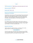
User’s Guide
Publication Number 01660-97017
First Edition, November 1995
For Safety Information, Warranties, and Regulatory Information, see the
pages at the end of this manual.
 Copyright Hewlett-Packard Company 1991 - 1995
All Rights Reserved.
HP 1660CS-Series
Logic Analyzers
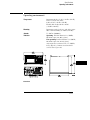
HP 1660CS-Series Logic Analyzers
The HP 1660CS-series logic analyzers are 100-MHz state/500-MHz
timing logic analyzers and 1 GSa/s digitizing oscilloscopes.
Logic Analyzer Features
• 130 data channels and 6 clock/data channels in the HP 1660CS
• 96 data channels and 6 clock/data channels in the HP 1661CS
• 64 data channels and 4 clock/data channels in the HP 1662CS
• 32 data channels and 2 clock/data channels in the HP 1663CS
• 3.5-inch flexible disk drive and 540 MB hard disk drive
• HP-IB, RS-232-C, and Centronics interfaces
• Variable setup/hold time
• 4 K memory on all channels with 8 K in half-channel mode
• Marker measurements
• 12 levels of trigger sequencing for state and 10 levels of trigger
sequencing for timing
• 100 MHz time tagging and number-of-states tagging
• Full programmability
• DIN mouse and keyboard support
Oscilloscope Features
• 8000 samples per channel
• Automatic pulse parameters
displays time between markers, acquires until specified time
between markers is captured, performs statistical analysis on
time between markers
• Lightweight miniprobes
Options include Ethernet LAN Interface, Programmer’s Guide, and
Service Guide
ii
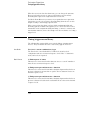
In This Book
This User’s Guide shows you how to
use the HP 1660CS-series logic
analyzer. It contains measurement
examples, field and feature
definitions, and a basic service guide.
Refer to this manual for information
on what the menu fields do and how
they are used. This manual covers all
HP 1660CS-series analyzers.
The User’s Guide is divided into four
parts. The first part, chapters 1
through 4, covers general product
information you need to use the logic
analyzer. The second part, chapters
5 and 6, contains detailed examples
to help you use your analyzer in
performing complex measurements.
The third part, chapters 7 through 9,
contains reference information on the
hardware and software, including the
analyzer menus and how they are
used. There are sections for each
analyzer menu and a separate
chapter on System Performance
Analysis. The fourth part, chapters 10
through 12, provides a basic service
guide.
1
The Logic Analyzer at a Glance
2
Connecting Peripherals
3
Using the Logic Analyzer
4
Using the Trigger Menu
5
Triggering Examples
6
File Management
7
Reference
8
System Performance Analysis
(SPA) Software
9
Concepts
10
Troubleshooting
11
Specifications
12
Operator’s Service
Glossary
Index
iii
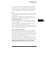
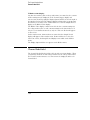
Introduction
iv
Contents
1 Logic Analyzer Overview
To make a measurement 1–4
2 Connecting Peripherals
To connect a mouse 2–3
To connect a keyboard 2–4
To connect to an HP-IB printer 2–5
To connect to an RS-232-C printer 2–7
To connect to a parallel printer 2–8
To connect to a controller 2–9
3 Using the Logic Analyzer
Accessing the Menus 3–3
To access the System menus 3–4
To access the Analyzer menus 3–6
To access the Scope menus 3–8
Using the Analyzer Menus 3–10
To label channel groups 3–10
To create a symbol 3–12
To examine an analyzer waveform 3–14
To examine an analyzer listing 3–16
To compare two listings 3–18
The Inverse Assembler 3–20
To use an inverse assembler
3–20
v
Contents
4 Using the Trigger Menu
Specifying a Basic Trigger 4–3
To assign terms to an analyzer 4–4
To define a term 4–5
To change the trigger specification 4–6
Changing the Trigger Sequence 4–7
To add sequence levels 4–8
To change macros 4–9
Setting Up Time Correlation between Analyzers 4–10
To set up time correlation between two state analyzers 4–11
To set up time correlation between a timing and a state analyzer 4–11
Arming and Additional Instruments 4–12
To arm another instrument 4–12
To arm the oscilloscope with the analyzer 4–13
To receive an arm signal from another instrument 4–15
Managing Memory 4–16
To selectively store branch conditions (State only) 4–17
To place the trigger in memory 4–18
To set the sampling rates (Timing only) 4–19
vi
Contents
5 Triggering Examples
Single-Machine Trigger Examples 5–3
To store and time the execution of a subroutine 5–4
To trigger on the nth iteration of a loop 5–6
To trigger on the nth recursive call of a recursive function 5–8
To trigger on entry to a function 5–10
To capture a write of known bad data to a particular variable 5–11
To trigger on a loop that occasionally runs too long 5–12
To verify correct return from a function call 5–13
To trigger after all status bus lines finish transitioning 5–14
To find the nth assertion of a chip select line 5–15
To verify that the chip select line is strobed after the address is stable 5–16
To trigger when expected data does not appear when requested 5–17
To test minimum and maximum pulse limits 5–18
To detect a handshake violation 5–20
To detect bus contention 5–21
Cross-Arming Trigger Examples 5–22
To examine software execution when a timing violation occurs 5–23
To look at control and status signals during execution of a routine 5–24
To detect a glitch 5–25
To capture the waveform of a glitch 5–26
To view your target system processing an interrupt 5–27
To trigger timing analysis of a count-down on a set of data lines 5–28
To monitor two coprocessors in a target system 5–29
Special displays 5–30
To interleave trace lists 5–31
To view trace lists and waveforms on the same display 5–32
vii
Contents
6 File Management
Transferring Files Using the Flexible Disk Drive 6–3
To save a configuration 6–4
To load a configuration 6–6
To save a listing in ASCII format 6–7
To save a screen’s image 6–8
To load additional software 6–9
7 Reference
Configuration Capabilities 7–3
Probing 7–5
General-purpose probing system description 7–8
Oscilloscope probes 7–11
Assembling the probing system 7–12
Keyboard Shortcuts 7–16
Moving the cursor 7–16
Entering data into a menu 7–17
Using the keyboard overlays 7–17
Common Menu Fields 7–18
Print field 7–19
Run/Stop field 7–20
Roll fields 7–21
Disk Drive Operations 7–22
Disk operations 7–22
Autoload 7–24
Format 7–24
Pack 7–24
Load and Store 7–25
viii
Contents
The RS-232-C, HP-IB, and Centronics Interfaces 7–26
The HP-IB interface 7–27
The RS-232-C interface 7–27
The Centronics interface 7–28
System Utilities 7–29
Real Time Clock Adjustments field 7–29
Update FLASH ROM field 7–29
Shade adjustments 7–30
The Analyzer Configuration Menu 7–31
Type field 7–31
Illegal configuration 7–31
The Analyzer Format Menu 7–32
Pod threshold field 7–32
State. acquisition modes (state only) 7–32
Timing acquisition modes (timing only) 7–33
Clock Inputs display 7–34
Pod clock field (State only) 7–34
Master and Slave Clock fields (State only) 7–37
Symbols field 7–40
Label fields 7–41
Label polarity fields 7–42
The Analyzer Trigger Menu 7–43
Trigger sequence levels 7–43
Modify trigger field 7–43
Timing trigger macro library 7–44
State trigger macro library 7–46
Modifying the user macro 7–48
Resource terms 7–51
Arming Control field 7–54
Acquisition Control field 7–56
Count field (State only) 7–57
ix
Contents
The Analyzer Listing Menu 7–58
Markers 7–58
The Analyzer Waveform Menu 7–60
sec/Div field 7–60
Accumulate field 7–60
Delay field 7–60
Waveform label field 7–61
Waveform display 7–62
The Analyzer Mixed Display Menu 7–63
Interleaving state listings 7–63
Time-correlated displays 7–64
Markers 7–64
The Analyzer Chart Menu 7–65
Min and Max scaling fields 7–66
Markers/Range field 7–66
The Analyzer Compare Menu 7–67
Reference Listing field 7–68
Difference Listing field 7–68
Copy Listing to Reference field 7–69
Find Error field 7–69
Compare Full/Compare Partial field 7–69
Mask field 7–70
Bit Editing field 7–70
Oscilloscope Common Menus 7–71
Run/Stop options 7–71
Autoscale 7–72
Time base 7–73
x
Contents
The Scope Channel Menu 7–74
Offset field 7–74
Probe field 7–75
Coupling field 7–75
Preset field 7–75
The Scope Display Menu 7–76
Mode field 7–76
Connect Dots field 7–77
Grid field 7–77
Display Options field 7–78
The Scope Trigger Menu 7–79
Trigger marker 7–79
Mode/Arm menu 7–79
Level field 7–81
Source field 7–82
Slope field 7–83
Count field 7–83
Auto-Trig field 7–84
When field 7–85
Count field 7–87
The Scope Marker Menu 7–88
Manual time markers options 7–88
Automatic time markers options 7–90
Manual/Automatic Time Markers option 7–94
Voltage Markers options 7–94
Channel Label field 7–96
The Scope Auto Measure Menu 7–97
Input field 7–97
Automatic measurements display 7–97
Automatic measurement algorithms 7–99
xi
Contents
8 System Performance Analysis (SPA) Software
System Performance Analysis Software 8–2
What is System Performance Analysis? 8–4
Getting started 8–6
SPA measurement processes 8–8
Using State Overview, State Histogram, and Time Interval 8–21
Using SPA with other features 8–30
9 Concepts
The File System 9–3
Directories 9–4
File types 9–5
Transitional Mode Theory 9–7
125-MHz transitional mode 9–7
250-MHz transitional mode 9–8
Other transitional timing considerations 9–11
The Trigger Sequence 9–12
Trigger sequence specification 9–13
Analyzer resources 9–15
Timing analyzer 9–18
State analyzer 9–18
Configuration Translation Between HP Logic Analyzers
The Analyzer Hardware 9–21
HP 1660CS-series analyzer theory 9–22
Logic acquisition board theory 9–25
Oscilloscope board theory 9–28
Self-tests description 9–32
xii
9–19
Contents
10 Troubleshooting
Analyzer Problems 10–3
Intermittent data errors 10–3
Unwanted triggers 10–3
No activity on activity indicators 10–4
Capacitive loading 10–4
No trace list display 10–4
Preprocessor Problems 10–5
Target system will not boot up 10–5
Slow clock 10–6
Erratic trace measurements 10–7
Inverse Assembler Problems 10–8
No inverse assembly or incorrect inverse assembly 10–8
Inverse assembler will not load or run 10–9
Error Messages 10–10
". . . Inverse Assembler Not Found" 10–10
"No Configuration File Loaded" 10–10
"Selected File is Incompatible" 10–10
"Slow or Missing Clock" 10–11
"Waiting for Trigger" 10–11
"Must have at least 1 edge specified" 10–12
"Time correlation of data is not possible" 10–12
"Maximum of 32 channels per label" 10–12
"Timer is off in sequence level n where it is used" 10–13
"Timer is specified in sequence, but never started" 10–13
"Inverse assembler not loaded - bad object code." 10–13
"Measurement Initialization Error" 10–14
"Warning: Run HALTED due to variable change" 10–14
xiii
Contents
11 Specifications
Accessories 11–2
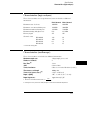
Specifications (logic analyzer) 11–3
Specifications (oscilloscope) 11–4
Characteristics (logic analyzer) 11–5
Characteristics (oscilloscope) 11–5
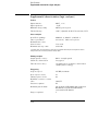
Supplemental characteristics (logic analyzer) 11–6
Supplemental characteristics (oscilloscope) 11–9
Operating environment 11–13
12 Operator’s Service
Preparing For Use 12–3
To inspect the logic analyzer 12–4
To apply power 12–4
To set the line voltage 12–5
To degauss the display 12–6
To clean the logic analyzer 12–6
To test the logic analyzer 12–6
Calibrating the oscilloscope 12–7
Set up the equipment 12–7
Load the default calibration factors 12–8
Self Cal menu calibrations 12–9
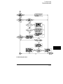
Troubleshooting 12–11
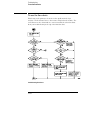
To use the flowcharts 12–12
To check the power-up tests 12–14
To run the self-tests 12–15
To test the auxiliary power 12–22
xiv
1
Logic Analyzer Overview
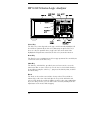
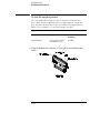
HP 1660CS-Series Logic Analyzer
Select Key
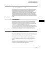
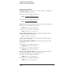
The Select key action depends on the type of field currently highlighted. If
the field is an option field, the Select key brings up an option menu or, if
there are only two possible values, toggles the value in the field. If the
highlighted field performs a function, the Select key starts the function.
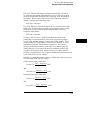
Done Key
The Done key saves assignments and closes pop-up menus. In some fields, its
action is the same as the Select key.
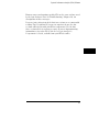
Shift Key
The shift key, which is blue, provides lowercase letters and access to the
functions in blue on some of the keys. You do not need to hold the shift key
down while pressing the other key — just press the shift key first, and then
the function key.
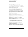
Knob
The knob can be used in some fields to change values. These fields are
indicated by a side view of the knob placed on top of the field when it is
selected. The knob also scrolls the display and moves the cursor within lists.
If you are using a mouse, you can do the same actions by holding down the
right button of the mouse while dragging.
1-2
Logic Analyzer Overview
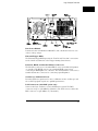
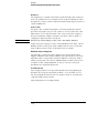
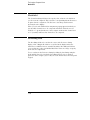
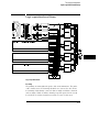
Line Power Module
Permits selection of 110-120 or 220-240 Vac and contains the fuses for each
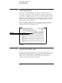
of these voltage ranges.
External Trigger BNCs
The External Trigger BNCs provide the "Port In" and "Port Out" connections
for the Arm In and Arm Out of the Trigger Arming Control menu.
RS-232-C, HP-IB, and Parallel Printer Connectors
The RS-232-C connector is a standard DB-25 connector for RS-232-C printer
or controller. The HP-IB connector is a standard HP-IB connector for
connecting an HP-IB printer or controller. The Parallel Printer connector is a
standard Centronics connector for connecting a parallel printer.
Oscilloscope Calibration Ports
Provides signals for operational accuracy calibration for the oscilloscope and
the oscilloscope/probe together to optimize performance.
LAN Connectors (with LAN option only)
Connects the logic analyzer to your local Ethernet network. The BNC
connector on top accepts 10Base2 ("thinlan"). The UTP connector below the
BNC connector accepts 10Base-T ("ethertwist").
1-3
Logic Analyzer Overview
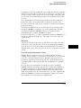
To make a measurement
To make a measurement
For more detail on any of the information below, see the referenced chapters
or the Logic Analyzer Training Kit. If you are using a preprocessor with the
logic analyzer, some of these steps may not apply.
Map to target
Connect probes Connect probes from the target system to the logic
analyzer to physically map the target system to the channels in the logic
analyzer. Attach probes to a pod in a way that keeps logically-related
channels together. Remember to ground the pod.
See Also
"Probing" in Chapter 7 for more detail on grounding and constructing probes.
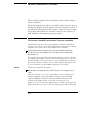
Set type* When the logic analyzer is turned on, Analyzer 1 is named
Machine 1 and is configured as a timing analyzer, and Analyzer 2 is off.
To use state analysis or software profiling, you must set the type of the
analyzer in the Analyzer Configuration menu. You can only use one
timing analyzer at a time.
Assign pods* In the Analyzer Configuration menu, assign the
connected pods to the analyzer you want to use. The number of pods on
your logic analyzer depends on the model. Pods are paired and always
assigned as a pair to a particular analyzer.
* If you load a configuration file, this step is not necessary.
1-4
Logic Analyzer Overview
To make a measurement
Set up analyzers*
Set modes and clocks Set the state and timing analyzers using the
Analyzer Format menu. In general, these modes trade channel count for
speed or storage. The state analyzer also provides for complicated
clocking. If your state clock is set incorrectly, the data gathered by the
logic analyzer might indicate an error where none exists.
See Also
"The Format Menu" in Chapter 7 for more information on modes and clocks.
Group bits under labels The Analyzer Format menu indicates active
pod bits. You can create groups of bits across pods or subgroups within
pods and name the groups or subgroups using labels.
* If you load a configuration file, this step is not necessary.
1-5
Logic Analyzer Overview
To make a measurement
Set up trigger*
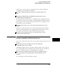
Define terms In the Analyzer Trigger menu, define trigger variables
called terms to match specific conditions in your target system. Terms
can match patterns, ranges, or edges across multiple labels.
Configure Arming Control Use Arming Control if
• you want to correlate the triggers and data of both analyzers
• you want to use the logic analyzer to trigger an external instrument or
the built-in oscilloscope, or
• you want to use an external instrument or the built-in oscilloscope to
trigger the logic analyzer.
Set up trigger sequence Create a sequence of steps that control when
the logic analyzer starts and stops storing data and filters which data it
will store. For common tasks, you can use a trigger macro to simplify the
process or use the user-defined macros to loop and jump in sequence.
You can also set the oscilloscope to trigger on a complex pattern.
See Also
Chapter 4,"Using the Trigger Menu" and Chapter 5, "Triggering Examples" for
more information on setting up a trigger.
"The Trigger Sequencer" in Chapter 9 for more information about the trigger
sequence mechanism.
"To save a configuration" and "To load a configuration" in Chapter 6 for
instructions on saving and loading the setup so you don’t have to repeat
setting up the analyzer and trigger.
* If you load a configuration file, this step is not necessary.
1-6
Logic Analyzer Overview
To make a measurement
Run measurement
Select single or repetitive From any Analyzer or Scope menu, select
the field labeled Run in the upper right corner to start measuring, or
press the Run key. A single run will run once, until memory is full; a
repetitive run will go until you select Stop or until a stop measurement
condition that you set in the markers menu is fulfilled.
See Also
"Markers Field" and "Scope Markers" in Chapter 7 for more information on
markers and stop measurement conditions.
If nothing happens, see Troubleshooting. When you start a run,
your analyzer menu changes to one of the display menus or a status
message pops up. If nothing happens, press the Stop key or select
Cancel. If the analyzer still does not display any measurements, see
Chapter 10, "Troubleshooting."
Gather data You can gather statistics automatically by going to a
Waveform or Listing menu, turning on markers, and setting patterns for
the X and O markers. You can set the logic analyzer to stop if certain
conditions are exceeded, or just use the markers to count valid runs.
See Also
"Markers Field," "Scope Markers," and "Scope Auto-measure" in Chapter 7 for
more information on markers.
1-7
Logic Analyzer Overview
To make a measurement
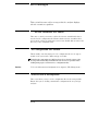
View data
Search for patterns In both the Waveform and Listing menus you can
use symbols and markers to search for patterns in your data. In the
Analyzer Waveform or Analyzer Listing menu, toggle the Markers field to
turn the pattern markers on and then specify the pattern. When you
switch views, the markers keep their settings.
Correlate data You can correlate data by setting Count Time in your
state analyzer’s Trigger menu and then using interleaving and mixed
display. Interleaving correlates the listings of two state analyzers. Mixed
display correlates a timing analyzer waveform and a state analyzer listing,
or a state analyzer and an oscilloscope waveform, or a state analyzer and
both timing and oscilloscope waveforms. To correlate oscilloscope data,
the oscilloscope arm mode must be set to Immediate. The System
Performance Analysis (SPA) Software does not save a record of actual
activity, so it cannot be correlated with either timing or state mode.
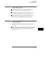
Make measurements The markers can count occurrences of events,
measure durations, and collect statistics, and SPA provides high-level
summaries to help you identify bottlenecks. To use the markers, select
the appropriate marker type in the display menu and specify the data
patterns for the marker. To use SPA, go to the SPA menu, select the
most appropriate mode, fill in the parameters, and press Run.
See Also
Chapter 8, "System Performance Analysis (SPA) Software" for more
information on using SPA.
"The Waveform Menu" and "The Listing Menu" in Chapter 7 for additional
information on the menu features.
1-8
2
Connecting Peripherals
Connecting Peripherals
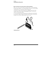
Your HP 1660CS-series logic analyzer comes with a PS2 mouse. It also
provides connectors for a keyboard, Centronics (parallel) printer, and
HP-IB and RS-232-C devices. This chapter tells you how to connect
peripheral equipment such as the mouse or a printer to the logic
analyzer.
Mouse and Keyboard
You can use either the supplied mouse and optional keyboard, or
another PS2 mouse and keyboard with standard DIN connector. The
DIN connector is the type commonly used by personal computer
accessories.
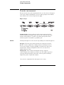
Printers
The logic analyzer communicates directly with HP PCL printers
supporting the printer control language or with other printers
supporting the Epson standard command set. Many non-Epson
printers have an Epson-emulation mode. HP PCL printers include the
following:
•
•
•
•
•
HP ThinkJet
HP LaserJet
HP PaintJet
HP DeskJet
HP QuietJet
You can connect your printer to the logic analyzer using HP-IB,
RS-232-C, or the parallel printer port. The logic analyzer can only
print to printers directly connected to it. It cannot print to a
networked printer.
2-2
Connecting Peripherals
To connect a mouse
To connect a mouse
Hewlett-Packard supplies a mouse with the logic analyzer. If you prefer a
different style of mouse you can use any PS2 mouse with a standard PS2 DIN
interface.
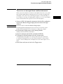
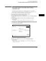
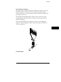
1 Plug the mouse into the mouse connector on the back panel. Make
sure the plug shows the arrow on top.
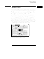
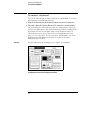
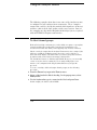
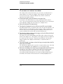
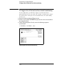
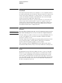
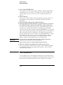
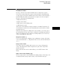
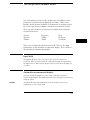
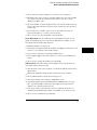
2 To verify connection, check the System External I/O menu for a
mouse box.
The mouse box is on the right side above the Settings fields. If the logic
analyzer was displaying the System External I/O menu when you plugged in
the mouse, the menu won’t update until you exit and then return to it.
The mouse pointer looks like a plus sign (+). To select a field, move the
pointer over it and press the left button. To duplicate the front-panel knob,
hold down the right button while moving the mouse. Moving the mouse up or
to the right duplicates turning the knob clockwise. Moving the mouse down
or to the left duplicates turning the knob counterclockwise.
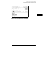
System External I/O menu showing mouse installed
2-3
Connecting Peripherals
To connect a keyboard
To connect a keyboard
You can use either the HP-recommended keyboard, HP E2427B, or any other
keyboard with a standard DIN connector.
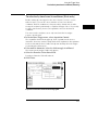
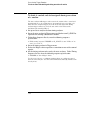
1 Plug the keyboard into the keyboard connector on the back panel.
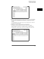
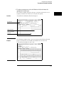
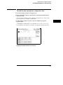
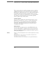
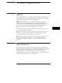
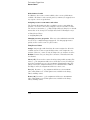
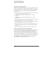
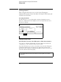
2 To verify, check the System External I/O menu for a keyboard box.
The keyboard box is on the right side, above the Settings fields. If the logic
analyzer was displaying the System External I/O menu while you plugged the
keyboard in, the menu won’t update until you exit and then return to it.
The keyboard cursor is the location on the screen highlighted in inverse
video. To move the cursor, use the arrow keys. Pressing Enter selects the
highlighted field. The primary keyboard keys act like the analyzer’s
front-panel data entry keys.
See Also
"Keyboard Shortcuts" in the Chapter 7 for complete key mappings.
System External I/O menu showing keyboard installed
2-4
Connecting Peripherals
To connect to an HP-IB printer
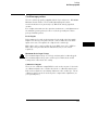
To connect to an HP-IB printer
Printers connected to the logic analyzer over HP-IB must support HP-IB and
Listen Always. When controlling a printer, the analyzer’s HP-IB port does not
respond to service requests (SRQ), so the SRQ enable setting does not have
any effect on printer operation.
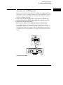
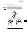
1 Turn off the analyzer and the printer, and connect an HP-IB cable
from the printer to the HP-IB connector on the analyzer rear panel.
2 Turn on the analyzer and printer.
3 Make sure the printer is set to Listen Always or Listen Only.
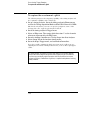
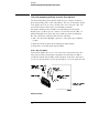
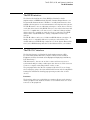
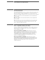
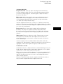
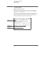
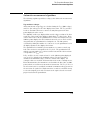
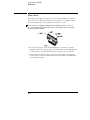
For example, the figure below shows the HP-IB configuration switches for an
HP-IB ThinkJet printer. For the Listen Always mode, move the second
switch from the left to the 1 position. Since the instrument doesn’t respond
to SRQ EN (Service Request Enable), the position of the first switch doesn’t
matter.
Listen Always switch setting
2-5
Connecting Peripherals
To connect to an HP-IB printer
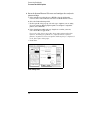
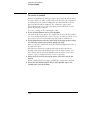
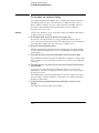
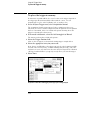
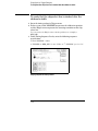
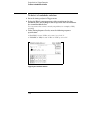
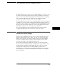
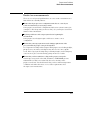
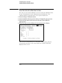
4 Go to the System External I/O menu and configure the analyzer’s
printer settings.
a If the analyzer is not already set to HP-IB, select the field under
b
c
d
e
Connected To: in the Printer box and choose HP-IB from the menu.
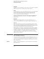
Select the Printer Settings field.
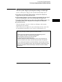
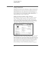
In the top field of the pop-up, select the type of printer you are using.
If you are using an Epson graphics printer or an Epson-compatible
printer, select Alternate.
If the default print width and page length are not what you want,
select the fields to toggle them.
If you select 132 characters per line when using a printer other than
QuietJet, the listings are printed in a compressed mode. QuietJet
printers can print 132 characters per line without going to compressed
mode, but require wider paper.
Press Done.
Printer Settings menu
2-6
Connecting Peripherals
To connect to an RS-232-C printer
To connect to an RS-232-C printer
1 Turn off the analyzer and the printer, and connect a null-modem
RS-232-C cable from the printer to the RS-232-C connector on the
analyzer rear panel.
2 Before turning on the printer, locate the mode configuration switches
on the printer and set them as follows:
• For the HP QuietJet series printers, there are two banks of mode function
switches inside the front cover. Push all the switches down to the 0
position.
• For the HP ThinkJet printer, the mode switches are on the rear panel of
the printer. Push all the switches down to the 0 position.
• For the HP LaserJet printer, the factory default switch settings are okay.
3 Turn on the analyzer and printer.
4 Go to the System External I/O menu and configure the analyzer’s
printer settings.
a If the analyzer is not already set to RS-232-C, select the field under
Connected To: in the Printer box and choose RS-232C from the menu.
b Select the Printer Settings field.
c In the top field of the pop-up, select the type of printer you are using.
If you are using an Epson graphics printer or an Epson-compatible
printer, select Alternate.
d If the default print width and page length are not what you want,
select the fields to toggle them.
If you select 132 characters per line when using a printer other than
QuietJet, the listings are printed in a compressed mode. QuietJet
printers can print 132 characters per line without going to compressed
mode, but require wider paper.
e Press Done.
5 Select the RS232 Settings field and check that the current settings are
compatible with your printer.
See Also
"The RS-232-C Interface" section in Chapter 7 for more information on
RS-232-C settings.
2-7
Connecting Peripherals
To connect to a parallel printer
To connect to a parallel printer
1 Turn off the analyzer and the printer, and connect a parallel printer
cable from the printer to the parallel printer connector on the
analyzer rear panel.
2 Before turning on the printer, configure the printer for parallel
operation.
The printer’s documentation will tell you what switches or menus need to be
configured.
3 Turn on the analyzer and printer.
4 Go to the System External I/O menu and configure the analyzer’s
printer settings.
a If the analyzer is not already set to Parallel, select the field under
b
c
d
e
Connected To: in the Printer box and choose Parallel from the menu.
Select the Printer Settings field.
In the top field of the pop-up, select the type of printer you are using.
If you are using an Epson graphics printer or an Epson-compatible
printer, select Alternate.
If the default print width and page length are not what you want,
select the fields to toggle them.
If you select 132 characters per line when using a printer other than
QuietJet, the listings are printed in a compressed mode. QuietJet
printers can print 132 characters per line without going to compressed
mode, but require wider paper.
Press Done.
There are no settings specific to the parallel printer connector.
2-8
Connecting Peripherals
To connect to a controller
To connect to a controller
You can control the HP 1660CS-series logic analyzer with another
instrument, such as a computer running a program with embedded analyzer
commands. The steps below outline the general procedure for connecting to
a controller using HP-IB or RS-232-C.
1 Turn off both instruments, and connect the cable.
If you are using RS-232-C, the cable must be a null-modem cable. If you do
not have a null-modem cable, you can purchase an adapter at any electronics
supply store.
2 Turn on the logic analyzer and then the controller.
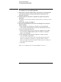
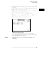
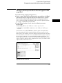
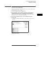
3 In the System External I/O menu, select the field under Connected
To: in the Controller box and set it appropriately.
The figure below is for HP-IB.
4 Select the appropriate Settings field and configure the values in the
pop-up menu to be compatible with the controller.
See Also
HP 1660C/CS-Series Logic Analyzers Programmer’s Guide and the LAN
User’s Guide for more information on connecting controllers.
2-9
2-10
3
Using the Logic Analyzer
Using the Logic Analyzer
This chapter shows you how to perform the basic tasks necessary to
make a measurement. Each section uses an example to show how the
task fits into the overall goal of making a measurement.
3–2
Accessing the Menus
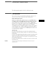
When you power up the logic analyzer, the first screen after the
system tests is the Analyzer Configuration menu. Menus are identified
by two fields in the upper left corner. The leftmost field shows
Analyzer. This field is sometimes referred to as the "mode field" or the
"module field" because it controls which other set of menus you can
access. The second field, just to the right of the mode field, accesses
menus within the mode and so is called the "menu field". Menus are
referred to by the titles that appear in the mode and menu fields, for
example, the Analyzer Configuration menu.
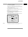
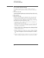
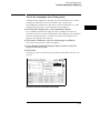
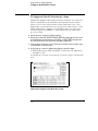
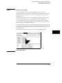
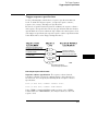
The figure below shows the top of the first screen. The mode field,
item 1, displays "Analyzer." The menu field, item 2, displays
"Configuration." Because menus are identified by the titles in these
two fields, this menu is referred to as the Analyzer Configuration
menu. When there is no risk of confusion, the menu is sometimes
referred to just by the title showing in the second field, for example,
the Configuration menu.
3–3
Using the Logic Analyzer
To access the System menus
To access the System menus
The System menus allow you to perform operations that affect the entire
logic analyzer, such as load configurations, change colors, and perform
system diagnostics.
1 Select the mode field.
Use the arrow keys to highlight the mode field, then press the Select key. Or,
if you are using the mouse, click on the field. This operation is referred to as
"select".
A pop-up menu appears with the choices System, Analyzer, and Scope. (If
you have installed any optional software, there may be other choices as well.)
2 Select System.
3 Select the menu field.
The pop-up lists five menus: Hard Disk, Flexible Disk, External I/O, Utilities,
and Test.
3–4
Using the Logic Analyzer
To access the System menus
• Hard Disk allows you to perform file operations on the hard disk
• Flexible Disk allows you to perform file operations on the flexible disk.
• External I/O allows you to configure your HP-IB, RS-232-C, and LAN
interfaces and connect to a printer and controller.
• Utilities allows you to set the clock, update the operating system software,
and adjust the display.
• Test displays the installed software version number and loads the self
tests.
See Also
For more information on operations available in the Disk menus, "File
Management" chapter and "Disk Drive Operations" in Chapter 7.
For more information on the External I/O, "Connecting Peripherals" chapter
and "The RS-232-C, HP-IB, and Centronics Interfaces" in Chapter 7.
For more information on the system utilities, "System Utilities" in Chapter 7.
For information on running the self-tests, "Operator’s Service" chapter.
3–5
Using the Logic Analyzer
To access the Analyzer menus
To access the Analyzer menus
The Analyzer menus allow you to control the analyzer to make your
measurement, perform operations on the data, and view the results on the
display.
1 Select the mode field.
A pop-up menu appears with the choices System, Analyzer, and Scope. (If
you have installed any optional software, there may be other choices as well.)
2 Select Analyzer.
3 Select the menu field.
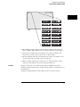
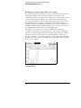
The figure on the next page shows all possible menus. Your analyzer will
never have all of them available at once, because certain menus are only
accessible with the analyzer configured in a particular mode. For instance,
the Compare menu is only available when you set an analyzer to state mode,
and the SPA menu requires an analyzer set to SPA.
• Configuration is always available in Analyzer mode. Use Configuration to
assign pods and set the analyzer type.
• Format is available whenever an analyzer is set to a type other than "Off."
Use Format to create data labels and symbols, adjust the pod threshold
level, and set modes and clocks.
• Trigger is available when an analyzer is set to State or Timing. Use Trigger
to specify a trigger sequence which will filter the raw information into the
measurement you want to see.
• Listing is available when an analyzer is set to State or Timing. Use Listing
to view your measurement as a list of states. Using an inverse assembler, a
state analyzer can display the measurement as though it were assembly
code.
• Compare is available only when an analyzer is set to State. Use Compare to
compare two listings and quickly scroll to the sections where they differ.
3–6
Using the Logic Analyzer
To access the Analyzer menus
• Mixed Display always appears in the menu list when an analyzer is set to
State or Timing, but it requires a State analyzer with time tags enabled.
• Waveform is available when an analyzer is set to State or Timing. Use
Waveform to view the data as logic levels on discrete lines.
• Chart is available only when an analyzer is set to State. Use Chart to view
your measurement as a graph of states versus time.
• SPA is available only when an analyzer is set to SPA. Use SPA to gather
and view overall statistics about your system performance.
See Also
Chapter 7, "Reference" for details on the State and Timing menus and
Chapter 8, "System Performance Analysis (SPA) Software" for information on
the SPA menu.
"Using the Analyzer Menus" in this chapter for how to use the menus.
3–7
Using the Logic Analyzer
To access the Scope menus
To access the Scope menus
The Scope menus allow you to control the analyzer to make your
measurement, perform operations on the data, and view the results on the
display.
1 Select the mode field.
A pop-up menu appears with the choices System, Analyzer, and Scope. (If
you have installed any optional software, there may be other choices as well.)
2 Select Scope.
3 Select the menu field.
The pop-up lists six menus: Scope Channel, Scope Display, Scope Trigger,
Scope Marker, Scope Auto Measure, and Scope Calibration.
• Scope Channel lets you select the channel input. It lets you set values that
control the vertical sensitivity, offset, probe attenuation factor, input
impedance, and coupling of the input channel currently shown in the Input
field. The Channel menu also gives you preset vertical sensitivity, offset,
and trigger level values for ECL and TTL logic levels.
• Scope Display controls how the oscilloscope acquires and displays
waveforms. You can acquire and display the waveforms in one of the
following modes: Normal, Average, or Accumulate. The Display options
also control the connect-the-dots display and grid display features.
3–8
Using the Logic Analyzer
To access the Scope menus
• Scope Trigger allows you to choose the method you want to use to trigger
the oscilloscope for a particular application. The three trigger modes are
Edge, Pattern, and Immediate.
• Scope Markers has two sets of markers that allow you to make time and
voltage measurements. These measurements can be made either manually
(voltage and time markers) or automatically (time markers only).
• Scope Auto Measure provides nine automatic measurements to fit the
acquired waveform to the display. These measurements are Period,
Risetime, Falltime, Frequency, +Width, −Width, Vp_p, Preshoot, and
Overshoot.
• Scope Calibration allows you to calibrate the oscilloscope or the
oscilloscope/probe system.
See Also
Chapter 12, "Operator’s Service," for details on calibrating the oscilloscope.
3–9
Using the Analyzer Menus
The following examples show how to use some of the Analyzer menus
to configure the logic analyzer for measurements. These examples
assume that you have already determined which signals are of interest
and have connected the logic analyzer to the target system. Some of
the examples use data from a Motorola 68360 target system, acquired
with an HP E2456A Preprocessor Interface.
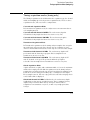
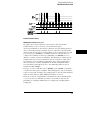
To label channel groups
Hewlett-Packard logic analyzers give you the ability to separate or group data
channels and label the groups with a name that is meaningful to your
measurement. Labels also assist you in triggering only on states of interest.
Labels can only be assigned in the Analyzer Format menu. Once assigned, the
labels are available in all display menus, where they can be added to or
deleted from the display. Use labels when you want to group data channels
by function with a name that has meaning to that function.
The default label names are Lab1 through Lab126. However, you can modify
a name to any six-character string. If you are using an HP preprocessor
interface, the configuration file has predefined labels for your specific
processor.
To create or modify a label and assign channel groups, use the following
procedure.
1 Press the Format key to go to the Format menu.
2 Select a label under the Labels heading. In the pop-up menu, select
Modify Label.
3 Use the keyboard to type in a name for the label and press Done.
In this example, the label is called CYCLE.
3–10
Using the Logic Analyzer
To label channel groups
4 Select the pod containing the channels for the label. Use the knob or
the arrow keys to position the selector over a channel you want to
change.
An asterisk indicates the channel is selected; a dot indicates the channel is
not part of the current group.
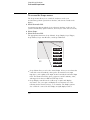
5 Toggle the channel’s group status by pressing Select.
The indicator changes and the selector moves to the next channel.
In this example, the channels 3, 1, and 0 (Pod A1) are assigned to label
CYCLE and the channels 6 and 3 (Pod A2) are assigned to the label Lab2.
3–11
Using the Logic Analyzer
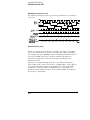
To create a symbol
To create a symbol
Symbols are alphanumeric mnemonics that represent specific data patterns
or ranges. When you define a symbol and set the the base type to Symbol in
the Listing menu, the symbol is displayed in the data listing where the bit
pattern would normally be displayed. The symbols also appear in the
Waveform menu when you view a label in bus form. Symbols allow you to
quickly identify data of interest.
To create a symbol, use the following procedure.
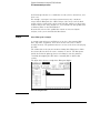
1 In the Analyzer Format menu, select Symbols.
The symbol table menu appears. The symbol table is where all user symbols
are created and maintained. If you get a message, "No labels specified," check
that you have at least one label turned on with channels assigned to it.
2 In the Symbol menu select the Label field. In the pop-up menu select
the label that contains the channel groups you want.
When you open the symbol table menu, the Label field displays the name of
the first active label.
If the label you want does not appear in the pop-up menu, the label is
probably off. Return to the Format menu, select the label you want, and
select Turn Label On. Another possibility is that the label is on the other
analyzer. The two analyzers manage resources separately.
3 Select the Base field. In the pop-up menu, select the base for the
pattern.
In this example, binary is used since CYCLE only contains three channels.
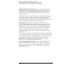
4 Select the field below Symbol. Select Add a Symbol, type in the
symbol name, then press Done.
3–12
Using the Logic Analyzer
To create a symbol
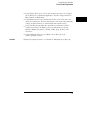
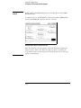
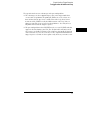
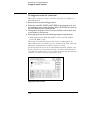
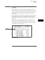
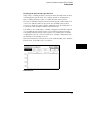
5 If additional Symbols are needed, repeat step 4 until you have added
all symbols.
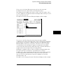
In this example three symbols are added: MEM RD, MEM WR, and DATA RD.
6 Toggle the Type field to "range" or "pattern".
When Type is range, a third field appears under the Stop column. To fully
specify a range, you need to enter a value for it, too.
7 Select the Pattern/Start field and use the keypad to enter an
appropriate value in the selected base. Use X for "don’t care."
8 When the pattern is specified, press Done. If you created additional
Symbols, repeat steps 6 and 7 until all symbols are specified.
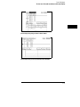
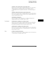
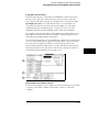
9 To close the symbol table menu, select Done.
Symbol table menu showing three symbols
You can also download symbol tables created by your programming
environment using HP E2450A Symbol Utility. The Symbol Utility is shipped
with the HP 1660CS-series logic analyzers.
See Also
HP E2450A Symbol Utility User’s Guide for more information on the
Symbol Utility.
3–13
Using the Logic Analyzer
To examine an analyzer waveform
To examine an analyzer waveform
The Analyzer Waveform menu allows you to view state or timing data in a
format similar to an oscilloscope display. The horizontal axis represents
states (in state mode) or time (in timing mode) and the vertical axis
represents logic highs and lows.
1 In Analyzer mode, press the Run key to acquire data.
In any mode other than Analyzer or Scope, pressing the Run key has no
effect. The menus which ignore Run lack the Run field onscreen. In Analyzer
mode with Run available, the menu changes to a display menu.
2 Go to the Analyzer Waveform menu.
3 To adjust the horizontal axis (sec/Div or states/Div) use the knob.
If nothing happens when you turn the knob, make sure the Div field has a roll
indicator above it, as in the figures on the next page. When you first enter
the Waveform menu, the knob adjusts the horizontal axis but if you select
another rollable field, the knob will control that field instead.
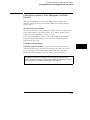
4 To adjust the display relative to the trigger, select the Delay field and
enter a value or use the knob.
The portion of memory being displayed is indicated by a white bar along the
bottom of the display area. The position of the trigger in memory is indicated
by a white dot on the same line. When the bar includes the dot, then the
trigger is visible on the display as indicated by a vertical line with a "t"
underneath.
5 To scroll through waveforms, select the large rectangle below the Div
field and use the knob.
The roll indicator appears at the top of the rectangle and the name of the first
waveform is highlighted. The highlight moves as you turn the knob.
6 To insert waveforms, select the large rectangle under the Div field. In
the pop-up, select Insert, and then select the labels and channels.
The Sequential field inserts all the channels of the label as individual
waveforms; the Bus field groups the waveforms; the Bit N field inserts just
the Nth bit. Waveforms are inserted after the currently highlighted one.
3–14
Using the Logic Analyzer
To examine an analyzer waveform
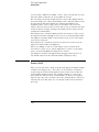
7 To take measurements, select the Markers field and choose the
appropriate marker type.
The markers available depend on the type of analyzer and whether or not
tagging is enabled. Use markers to locate patterns quickly.
See Also
"Count Field" and "Markers Field" in Chapter 7.
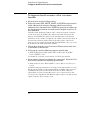
roll indicator
trigger indicator
memory displayed
indicator
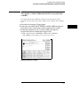
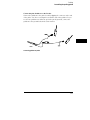
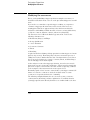
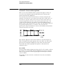
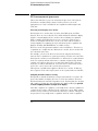
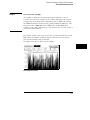
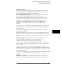
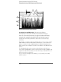
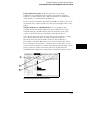
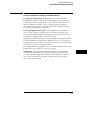
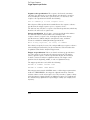
Example
The following example shows a state waveform from the Hewlett-Packard
preprocessor interface for the Motorola 68360. Notice how the bus
waveforms insert symbols or state data.
3–15
Using the Logic Analyzer
To examine an analyzer listing
To examine an analyzer listing
The Analyzer Listing menu displays state or timing data as patterns (states).
The Listing menu uses any of several formats to display the data such as
binary, ASCII, or symbols. If you are using an inverse assembler and select
Invasm, the data is displayed in mnemonics that closely resemble the
microprocessor source code.
See Also
"The Inverse Assembler" at the end of this chapter for additional information
on using an inverse assembler.
1 In Analyzer mode, press the Run key to acquire data.
In any mode other than Analyzer or Scope, pressing the Run key has no
effect. The menus which ignore Run lack the Run field onscreen. In Analyzer
mode with Run available, the menu changes to a display menu.
2 Go to the Analyzer Listing menu.
All labels defined in the Analyzer Format menu appear in the listing. If there
are more labels than will fit on the screen, the Label/Base field is shaded like
a normal field.
3 To scroll the labels, select the Label/Base field and use the knob.
If the Label/Base field is selectable, the roll indicator appears over the field as
in the example. To move the labels one full screen at a time, press Shift and
a Page key.
4 To scroll the data, use the Page keys or select the data roll field and
use the knob.
If you select the data roll field, the roll indicator moves to it. No matter
which field is currently controlled by the knob, however, the Page keys page
the data up or down.
The numbers in the data roll column indicate how many samples the data is
from the trigger. Negative numbers occurred before the trigger and positive
numbers occurred after.
5 If the labels have symbols associated with them, set the base to
Symbol.
The symbols you defined appear in the listing.
3–16
Using the Logic Analyzer
To examine an analyzer listing
6 To insert a label, select one of the label fields, then select Insert from
the pop-up and the label you want to insert.
The last label cannot be deleted, so there is always at least one label. You can
insert the same label multiple times and display it in different bases.
7 To take measurements, select the Markers field and choose the
appropriate marker type.
The markers available depend on the type of analyzer and whether or not
tagging is enabled. Use markers to locate states quickly.
See Also
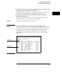
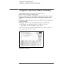
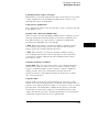
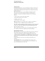
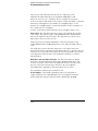
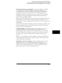
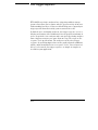
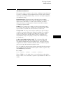
Example
"Count Field" and "Markers Field" in Chapter 7.
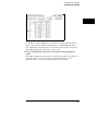
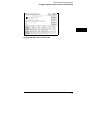
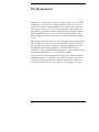
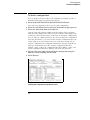
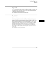
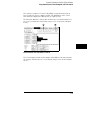
The following illustration shows a listing from the Hewlett-Packard
preprocessor interface for the Motorola 68360. The ADDR label has the base
set to Hex to conserve space on the display. The DATA label has the base set
to Invasm for inverse assembly. The FC label has the base set to Symbol.
Additional labels are located to the right of FC, and can be viewed by
highlighting and selecting Label, then using the knob to scroll the display
horizontally.
roll indicator
data roll field
3–17
Using the Logic Analyzer
To compare two listings
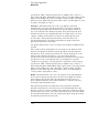
To compare two listings
The Compare menu allows you to take two state analyzer acquisitions and
compare them to find the differences. You can use this function to quickly
find all the effects after changing the target system or to quickly compare the
results of quality tests with results from a working system.
1 In Analyzer mode, press the Run key to acquire data.
In any mode other than Analyzer or Scope, pressing the Run key has no
effect. The menus which ignore Run lack the Run field onscreen. In Analyzer
mode with Run available, the menu changes to a display menu.
2 Go to the Analyzer Compare menu, select Copy Listing to Reference,
and then select Execute.
The Compare menu initially is empty, but when you select Execute the data
appears.
3 Set up the other test that you want to compare to the first.
This can be a change to the hardware, or a different system. Do not change
the trigger, however, or all the states will be different.
4 Run the test again, then select the Reference listing field to toggle to
Difference listing.
The Difference listing is displayed on the next page.
3–18
Using the Logic Analyzer
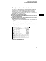
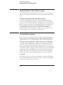
To compare two listings
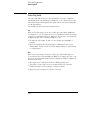
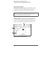
The Difference listing displays the states that are identical in dark typeface,
and the states that are different in light typeface (indistinguishable in the
above illustration). The light typeface shows the data from the compare file
that is different from the data in the reference file.
5 Select the Find Error field and use the knob to scroll through the
errors.
The display jumps past all states that are identical, and shows the number of
errors through the current state in the Find Error field. In the above
illustration, there are 37 errors through state 44 of the listing.
3–19
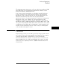
The Inverse Assembler
When the analyzer captures a trace, it captures binary information.
The analyzer can then present this information in symbol, binary,
octal, decimal, hexadecimal, or ASCII. Or, if given information about
the meaning of the data captured, the analyzer can inverse assemble
the trace. The inverse assembler makes the trace list more readable
by presenting the trace results in terms of processor opcodes and data
transactions.
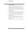
To use an inverse assembler
Most preprocessors include an inverse assembler in their software. Loading
the configuration file for the preprocessor sets up the logic analyzer to
provide certain types of information for the inverse assembler. This section
is provided in case you ever have to set up an analyzer for inverse assembly
yourself.
The inverse assembly software needs at least these five pieces of information:
• Address bus. The inverse assembler expects to see the label ADDR, with
bits ordered in a particular sequence.
• Data bus. The inverse assembler expects to see the label DATA, with bits
ordered in a particular sequence.
• Status. The inverse assembler expects to see the label STAT, with bits
ordered in a particular sequence.
• Start state for disassembly. This is the first displayed state in the trace list,
not the cursor position. See the figure on the next page.
• Tables indicating the meaning of particular status and data combinations.
The particular sequences that each label requires depends on the type of
chip the inverse assembler was designed for. Because of this, inverse
assemblers cannot generally be transferred between platforms.
To run the inverse assembler, you must be sure the labels are spelled
correctly as shown here, or as directed in your inverse assembler
documentation. Even a minor difference such as not capitalizing each letter
will cause the inverse assembler to not work.
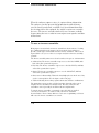
3–20
Using the Logic Analyzer
To use an inverse assembler
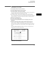
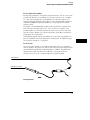
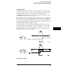
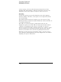
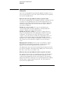
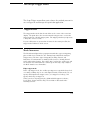
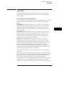
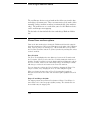
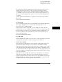
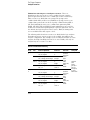
The inverse assembler
synchronizes at the
first line in the trace
list...
not at the cursor
position
Inverse assembly synchronization
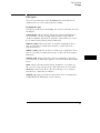
When you press the Invasm key to begin inverse assembly of a trace, the
inverse assembler begins with the first displayed state in the trace list. This is
called synchronization. It looks at the status bits (STAT) and determines
the type of processor operation, which is then displayed under the STAT
label. If the operation is an opcode fetch, the inverse assembler uses the
information on the data bus to look up the corresponding opcode in a table,
which is displayed under the DATA label. If the operation is a data transfer,
the data and corresponding operation are displayed under the DATA label.
This continues for all subsequent states in the trace list.
If you roll the trace list to a new position and press Invasm again, the inverse
assembler repeats the above process. However, it does not work backward in
the trace list from the starting position. This may cause differences in the
trace list above and below the point where you synchronized inverse
assembly. The best way to ensure correct inverse assembly is to synchronize
using the first state you know to be the first byte of an opcode fetch.
See Also
The Preprocessor User’s Guide for more information on controlling inverse
assembly.
"Troubleshooting," Chapter 10, if you have problems using the inverse
assembler.
3–21
3–22
4
Using the Trigger Menu
Using the Trigger Menu
To use the logic analyzer efficiently, you need to be able to set up your
own triggers. This book provides examples of triggering in the next
chapter. Those examples assume you already know where to find
fields in the trigger menu. This chapter explains how to use those
fields.
This chapter shows you how to:
•
•
•
•
•
Specify a basic trigger
Change a trigger sequence
Set up time correlation between analyzers
Arm from another instrument, or arm another instrument
Manage memory
Much of the information here is also covered in the Logic Analyzer
Training Kit, but this chapter presents the information in a more
general form.
4–2
Specifying a Basic Trigger
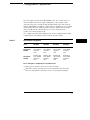
The default analyzer triggers are
While storing "anystate" TRIGGER on "a" 1 time
Store "anystate"
for state analyzers and
TRIGGER on "a" > 8 ns
for timing analyzers. The oscilloscope triggers separately from the
logic analyzers. If you want to simply record data, these will get you
started. They can quickly be tailored by specifying a particular pattern
to look for instead of the general case.
Customizing a trigger generally requires these steps:
• Assign terms to both analyzers
• Define the terms
• Change the trigger to use the new terms
The oscilloscope can be used in complex triggering sequences
managed by the logic analyzer, but its inherent trigger mechanism is
much simpler. Using the oscilloscope in conjunction with one or both
of the analyzers is covered in "Arming and Additional Instruments" in
this chapter. The different modes of triggering the oscilloscope are
covered in "The Scope Trigger Menu" in Chapter 7.
4–3
Using the Trigger Menu
To assign terms to an analyzer
To assign terms to an analyzer
When you turn the logic analyzer on, Analyzer 1 is named Machine 1 and
Analyzer 2 is off. Trigger terms can only be used by one analyzer at a time,
so all the terms are assigned to Analyzer 1. If you plan to use both analyzers
in your measurement, you need to assign some of the terms to Analyzer 2.
1 Go to the Trigger Machine 1 menu.
If you have renamed Machine 1 in the Analyzer Configuration menu, the
name you changed it to will appear in the menu instead of Machine 1.
2 Select a term.
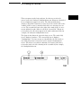
The terms are the fields below the roll field "Terms". See the figure below.
Terms
3 Select Assign from the list that appears.
The Resource Term Assignment menu appears. It is divided into two
sections, one for each analyzer. All the terms are listed.
4 To change a term assignment, select the term field.
The term fields toggle from one section to the other. You can get all your
terms assigned at once, or just change a few to meet immediate needs.
5 To exit the term assignment menu, select Done.
4–4
Using the Trigger Menu
To define a term
To define a term
Both default triggers trigger on term "a". If you only need to look for the
occurrence of a certain state, such as a write to protected memory, then you
only need to define term "a" to make the measurement you want.
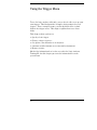
1 In the Trigger menu, select the field at the intersection of the term
and the label whose value you want to trigger on.
You set labels in the Analyzer Format menu. If the channels you want to
monitor are not attached to a label, they will not appear in the trigger menu.
2 Enter the value or pattern you want to trigger on.
If the label’s base is Symbol, a pop-up menu appears offering a choice of
symbols. For other bases, use the keypad. An "X" stands for "don’t care".
If there are two conditions that need to be present at the same time, for
example a protected address on the address bus and a write on the read/
write line, define both values on the same term. See the figure below.
3 Press Done.
Term "a" defined as a data write to read-only memory
4–5
Using the Trigger Menu
To change the trigger specification
To change the trigger specification
Most triggers use terms other than "a." Even a simple trigger might use
additional terms to set conditions on the actual trigger. To use these terms,
you must include them in the trigger sequence specification.
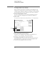
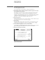
1 In the Trigger menu, select the number beside the specific level you
want to modify.
A Sequence Level menu pops up. It shows the current specification for that
trigger level.
2 Select the field you want to change.
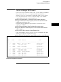
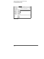
In the top row of the pop-up are three action fields: Insert Level, Select New
Macro, and Delete Level. The next section goes into detail on them. The
fields after "While storing," "TRIGGER on," and "Else on" are completed with
trigger terms. Selecting these fields pops up a menu of terms(see below).
3 Select the term you want to use from the pop-up, or enter a new
value, as appropriate to the field.
Selecting "Combination" pops up a menu to define a term combination. The
combination mechanism is discussed in "Resource Terms" in Chapter 7 and
"The Trigger Sequencer" in Chapter 9.
If you have renamed a term, that name is automatically used everywhere the
term would appear.
4 Select Done until you are back at the Trigger menu.
Term selection pop-up menu
4–6
Changing the Trigger Sequence
Most measurements require more complicated triggers to better filter
information. From the basic trigger, you can
• Add sequence levels
• Change macros
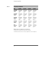
Your logic analyzer provides a macro library to make setting up the
trigger easier. There are 12 state macros and 13 timing macros. Most
macros take more than one level internally to implement, and can be
broken down into their separate levels. Once broken down, the levels
can be used to design your own trigger sequences.
4–7
Using the Trigger Menu
To add sequence levels
To add sequence levels
You can add sequence levels anywhere except after the final one.
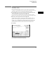
1 In the Trigger menu, select the number beside the sequence level just
after where you want to insert.
For example, if you want to insert a sequence level between levels 1 and 2,
you would select level 2. To insert levels at the beginning, select level 1.
A Sequence Level pop-up appears. Its exact contents depend on the analyzer
configuration and the level specification. However, all Sequence Level
pop-ups have an Insert Level field in the upper left corner.
2 Select Insert Level.
Another pop-up offers the choices of Cancel, Before, or After. If the level you
started from was the last level, After will not appear.
3 Select Before.
The Trigger Macro pop-up replaces the Sequence Level pop-up. The macros
available depend on whether the analyzer is configured as state or timing.
4 Use the knob to highlight a macro, and select Done.
A new Sequence level pop-up appears. Its contents reflect the macro you just
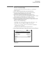
selected. The figure below shows a user macro for a state analyzer.
5 Fill in the fields and select Done.
Sequence Level pop-up menu
4–8
Using the Trigger Menu
To change macros
To change macros
You do not need to add and delete levels just to change a level’s macro. This
can be done from within the Sequence Level pop-up.
1 From the Trigger menu, select the sequence level number of the
sequence level you want to modify.
A Sequence Level pop-up appears. Its contents reflect the current macro.
2 Select Select New Macro.
The Trigger Macro pop-up replaces the Sequence Level pop-up. The macros
available depend on whether the analyzer is configured as state or timing.
3 Use the knob to highlight the macro you want, and select Done.
A new Sequence Level pop-up appears. Its contents reflect the macro you
just selected. The wording of this screen is very similar to the macro
description, and the line drawing demonstrates what the macro is measuring.
4 Select the appropriate assignment fields and insert the desired
pre-defined terms, numeric values, and other parameter fields
required by the macro. Select Done.
See Also
"Timing Trigger Macro Library" and "State Trigger Macro Library" in
Chapter 7 for a complete listing of macros.
4–9
Setting Up Time Correlation between Analyzers
There are two possible combinations of analyzers: state and state, and
state and timing. Timing and timing is not possible because the
Analyzer Configuration menu only permits one analyzer at a time to
be configured as a timing analyzer. For either combination, time
correlation is necessary for interleaving and mixed display.
Time correlation is useful when you want to store different sorts of
data for each trace, but see how they are related. For instance, you
could set up a timing and a correlated state analyzer and see if setup
and hold times are being met. Or, you could set up two state analyzers
and have one watch normal program execution and the other watch
the control and status lines.
Time correlation requires that state analyzers store time tags. You set
the state analyzer to store time tags by turning on Count Time in the
Analyzer Trigger menu. The timing analyzer already stores time tags
when it samples data.
See Also
"Special Displays" in Chapter 5 for more information on interleaving
and mixed display.
4–10
Using the Trigger Menu
To set up time correlation between two state analyzers
To set up time correlation between two state analyzers
To correlate the data between two state analyzers, both must have Count
Time turned on in their Trigger menus. Although both have Count State
available, it is not possible to correlate data based on states even when they
are identically defined.
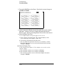
1 In the Analyzer Trigger menu, select Count.
Count may be Count Off, Count Time, or Count States. Selecting the field
causes a pop-up to appear.
2 Select the field after Count: and select Time.
A warning may appear about reduced memory. It will not prevent you from
changing Count to Count Time.
3 Select Done.
4 Repeat steps 1 through 3 for the other state analyzer.
Now when you acquire data you will be able to interleave the listings.
To set up time correlation between a timing and a
state analyzer
To set up time correlation between a timing and a state analyzer, only the
state analyzer needs to have Count Time turned on. The timing analyzer
automatically keeps track of time.
1 In the state Analyzer Trigger menu, select Count.
Count may be Count Off, Count Time, or Count States. Selecting the field
causes a pop-up to appear.
2 Select the field after Count: and select Time.
A warning may appear about reduced memory. It will not prevent you from
changing Count to Count Time.
3 Select Done.
Now when you acquire data you will be able to set up a mixed display.
4–11
Arming and Additional Instruments
Occasionally you may need to start the analyzer acquiring data when
another instrument detects a problem. Or, you may want to have the
analyzer itself arm another measuring tool. This is accomplished from
the Arming Control field of the Analyzer Trigger menu.
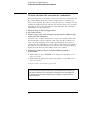
To arm another instrument
1 Attach a BNC cable from the External Trigger Output port on the
back of the logic analyzer to the instrument you want to trigger.
The External Trigger Output port is also referred to as "Port Out." It uses
standard TTL logic signal levels, and will generate a rising edge when trigger
conditions are met.
2 In the Analyzer Trigger menu, select Arming Control.
Arming Control is below the Run button.
3 Select the Port Out field, and choose Analyzer from the list.
4 If you are using both analyzers, set the Arm Out Sent From field in
the upper right corner.
This field does not appear if only one analyzer is configured.
The selected analyzer will send the arm signal when it finds its trigger.
5 Select Done.
When you make a measurement, the analyzer will send an arm signal through
the External Trigger Output when the analyzer finds its trigger.
4–12
Using the Trigger Menu
To arm the oscilloscope with the analyzer
To arm the oscilloscope with the analyzer
If both analyzers and the oscilloscope are turned on, you can configure one
analyzer to arm the other analyzer and the oscilloscope. An example of this
is when a state analyzer triggers on a bit pattern, then arms a timing analyzer
and the oscilloscope which capture and display the waveform after they
trigger.
1 In the Analyzer Trigger menu, select Arming Control.
2 Select the Analyzer Arm Out Sent From field, and choose from the
list the Analyzer that will generate the arm.
3 Select the Analyzer Arm In field, and choose Group Run.
This allows you to time-correlate the data from the analyzers and the scope.
The Scope Trigger Mode must be Immediate for correlation.
4 Select the field of the instrument which will arm the others, and in
the pop-up set it to run from Group Run.
The Scope field is not selectable. To set how the scope is run, select the field
under Scope Arm In.
5 Select the other instrument fields and choose the mechanism which
will arm them.
The Analyzer Arm Out field determines which analyzer sends the arming
signal to Port Out and to the oscilloscope if the oscilloscope is being armed
by an analyzer.
As you set each machine, the arrows connecting the fields in the Arming
Control menu change. The arrows show the order in which the instruments
are armed.
See the example on the next page.
6 Select Done until you are back at the Trigger menu.
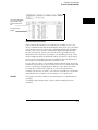
4–13
Using the Trigger Menu
To arm the oscilloscope with the analyzer
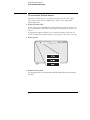
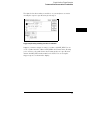
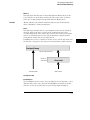
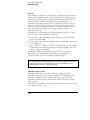
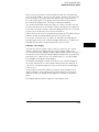
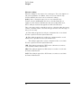
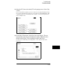
Example
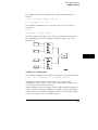
In this example STATE MACH triggers from Group Run, then arms TIME
MACH and Scope.
To duplicate this, set STATE MACH to run from Group Run, TIME MACH to
run from STATE MACH, and Scope Arm In to Analyzer.
Arming with two analyzers and an oscillscope
When the run starts, the state analyzer automatically begins evaluating its
trigger sequence instruction. When the trigger sequence is satisfied, the
state analyzer sends an "Arm" signal to the timing analyzer, the oscilloscope,
and the external trigger.
4–14
Using the Trigger Menu
To receive an arm signal from another instrument
To receive an arm signal from another instrument
When you set the analyzer to wait for an arm signal, it does not react to data
that would normally trigger it until after it has received the arm signal. The
arm signal can be sent to any of the Trigger Sequence levels, but will go to
level 1 unless you change it. Setting up the analyzer to receive an arm signal
is more efficient when the sequence levels are already in place.
1 Connect a BNC cable from the instrument which will be sending the
signal to the External Trigger Input port on the back of the logic
analyzer.
CAUTION
Do not exceed 5.5 volts on the External Trigger Input.
The External Trigger Input port is also referred to as "Port In." It uses
standard TTL logic signal levels, and expects a rising edge as input.
2 In the Analyzer Trigger menu, select Arming Control.
Arming Control is below the Run button.
3 Select the Analyzer Arm In field, and choose PORT IN.
4 To change the default settings, select the analyzer field.
A small pop-up menu appears. To change which device the analyzer is
receiving its arm signal from, select the Run from field. To change which
sequence level is waiting for the arm signal, select the Arm sequence level
field.
5 Select Done until you are back at the Trigger menu.
4–15
Managing Memory
Sometimes you will need every last bit of memory you can get on the
logic analyzer. There are three simple ways to maximize memory
when specifying your trigger:
• Selectively store branch conditions (State only)
• Place the trigger relative to memory
• Set the sampling rates (Timing only)
4–16
Using the Trigger Menu
To selectively store branch conditions (State only)
To selectively store branch conditions (State only)
Besides setting up your trigger levels to store anystate, no state, or some
subset of states, you can also choose whether or not to store branch
conditions. Branch conditions are always stored by default, and can make
tracing the analyzer’s path through a complicated trigger easier. If you really
need the extra memory, however, it is possible to not store the branch
conditions.
You cannot set the analyzer to store only some branches in a trigger
sequence specification.
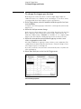
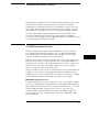
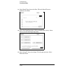
1 In the Analyzer Trigger menu, select Acquisition Control.
The Acquisition Control menu pops up. If the acquisition mode is set to
Automatic, the menu contains a single field and an explanation. If Acquisition
has been customized, it has 3 fields and a picture showing where the trigger
is currently placed in memory.
2 If the mode is Automatic, select the field to toggle it to Manual.
The menu now shows three fields and a picture.
3 Select the Branches Taken Stored field.
It toggles to Branches Taken Not Stored.
4 Select Done.
Acquisition Control menu with branches field highlighted
4–17
Using the Trigger Menu
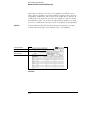
To place the trigger in memory
To place the trigger in memory
In Automatic Acquisition Mode, the exact location of the trigger depends on
the trigger specification but usually falls around the center. You can
manually place it to be at the beginning, end, or anywhere else.
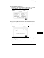
1 In the Analyzer Trigger menu, select Acquisition Control.
The Acquisition Control menu pops up. If the acquisition mode is set to
Automatic, the menu contains a single field and an explanation. If Acquisition
has been customized, it has 3 or 4 fields and a picture showing where the
trigger is currently placed in memory.
2 If the mode is Automatic, select the field to toggle it to Manual.
The menu now shows three fields and a picture.
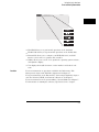
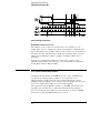
3 Select the Trigger Position field.
A list of choices appears, as shown in the timing trigger example below.
4 Select the appropriate entry for your needs.
Start, Center, and End place the trigger respectively at the beginning, middle,
and end of the memory. Delay, available in timing analyzers only, causes the
analyzer to not save any data before the time delay has elapsed. User Defined
calls up a fourth field where you specify exactly where you want the trigger.
5 Select Done.
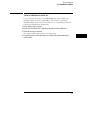
Acquisition Control menu with trigger position pop-up for a timing analyzer
4–18
Using the Trigger Menu
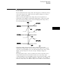
To set the sampling rates (Timing only)
To set the sampling rates (Timing only)
A timing analyzer samples the data based on its own internal clock. A short
sample period provides more detail about the device under test; a
long sample period allows more time before memory is full. However, if the
sample period is too large, some information may be missed.
1 In the Analyzer Trigger menu, select Acquisition Control.
The Acquisition Control menu pops up. If the acquisition mode is set to
Automatic, the menu contains a single field and an explanation. If Acquisition
has been customized, it has 3 or 4 fields and a picture showing where the
trigger is currently placed in memory.
2 If the mode is Automatic, select the field to toggle it to Manual.
The menu now shows three fields and a picture.
3 Set the Sample Period field using the knob, or select it to use the
keypad to enter the period.
4 Select Done.
Next time you take a measurement, the analyzer will sample at the rate you
entered.
Acquisition Control menu with Sample Period selected
4–19
4–20
5
Triggering Examples
Triggering Examples
As you begin to understand a problem in your system, you may realize
that certain conditions must occur before the problem occurs. You
can use sequential triggering to ensure that those conditions have
occurred before the analyzer recognizes its trigger and captures
information.
If you are not familiar with the trigger menus, read through the
previous chapter, "Using the Trigger Menu," and try working through
the examples in the Logic Analyzer Training Kit manual.
5-2
Single-Machine Trigger Examples
The following examples require only a single analyzer to make
measurements. Sequence specifications are given in the form you see
within the sequence levels, but the illustrations show the complete,
multi-level sequence specification.
Although all the examples are case-specific, terms are named in a way
that highlights their role in solving the trigger problem. You can easily
apply the examples to your specific instance by changing the specific
values assigned to the trigger terms.
5-3
Single-Machine Trigger Examples
To store and time the execution of a subroutine
To store and time the execution of a subroutine
Most system software of any kind is composed of a hierarchy of functions and
procedures. During integration, testing, and performance evaluation, you
want to look at specific procedures to verify that they are executing correctly
and that the implementation is efficient. The analyzer allows you to do this by
triggering on entry to the address range of the subroutine and counting the
elapsed time since the trigger state.
1 Go to the state analyzer’s Trigger menu.
2 Set Count to Time.
3 Define a range term, such as Range1, to represent the address range
of the particular subroutine.
You may need to examine the structure of your code to help determine this.
If your subroutine calls are really procedure calls, then there is likely to be
some code at the beginning of the routine that adjusts the stack for local
variable allocation. This will precede the address of the first statement in the
procedure. If your subroutine has no local storage and is called by a jump or
branch, then the first statement will also be the entry address.
4 Under State Sequence Levels, enter the following sequence
specification:
• While storing "no state" TRIGGER on "In_Range1" Occurs 1 Else on "no
state" go to level 1
• While storing "In_Range1" Then find "Out_Range1" Occurs 1 Else on "no
state" go to level 2
• Store "no state" on "no state" go to level 1
For processors that prefetch instructions or have pipelined architectures, you
may want to add part or all of the depth of the pipeline to the start address for
In_Range1 to ensure that the analyzer does not trigger on a prefetched but
unexecuted state.
5-4
Single-Machine Trigger Examples
To store and time the execution of a subroutine
The figure below shows what you would see on your analyzer screen after
entering the sequence specification given in step 4.
Trigger setup for storing and timing execution of a subroutine
Suppose you want to trigger on entry to a routine called MY_SUB. You can
create a symbol from the address of MY_SUB in the Format menu, allowing
you to reference the symbol name when setting up the trace specification.
Assume that MY_SUB extends for 0A hex locations. You can set up the
trigger sequence as shown in the display.
5-5
Single-Machine Trigger Examples
To trigger on the nth iteration of a loop
To trigger on the nth iteration of a loop
Traditional debugging requires print statements around the area of interest.
This is not possible in most embedded systems designs, but the analyzer
allows you to view the system’s behavior when a particular event occurs.
Suppose that your system behaves incorrectly on the last iteration of a loop,
which, in this instance, happens to be the 10th iteration. You can use the
analyzer’s triggering capabilities to capture that iteration and subsequent
processor activity.
1 Go to the state analyzer’s Trigger menu.
2 Define the terms LP_START and LP_END to represent the start and
end addresses of statements in the loop, and LP_EXIT to represent
the first statement executed after the loop terminates.
3 Change State Sequence Level 1’s macro to "Find event2 n times after
event1 before event3 occurs."
4 In the pop-up, enter the following sequence specification:
• While storing anystate Find "LP_START" "9" times after "LP_END" before
"LP_EXIT" occurs.
You should use your value for n-1 instead of "9" in the sequence specification
above.
Trigger setup for triggering on the 10th iteration of a loop
5-6
Single-Machine Trigger Examples
To trigger on the nth iteration of a loop
The specification has some advantages and a potential problem.
• The advantages are that a pipelined processor won’t trigger until it has
executed the loop 10 times. Requiring LP_END to be seen at least once
first ensures that the processor actually entered the loop; then, 9 more
iterations of LP_START is really the 10th iteration of the loop. Also, no
trigger occurs if the loop executes less than 10 times – the analyzer sees
LP_EXIT and restarts the trigger sequence.
• The potential problem is that LP_EXIT may be too near LP_END and thus
appear on the bus during a prefetch. The analyzer will constantly restart
the sequence and will never trigger. The solution to this problem depends
on the structure of your code. You may need to experiment with different
trigger sequences to find one that captures only the data you want to view.
5-7
Single-Machine Trigger Examples
To trigger on the nth recursive call of a recursive function
To trigger on the nth recursive call of a recursive
function
1 Go to the state analyzer’s Trigger menu.
2 Define the terms CALL_ADD, F_START, and F_END to represent the
called address of the recursive function, and the start and end
addresses of the function. Define F_EXIT to represent the address of
the first program statement executed after the original recursive call
has terminated.
Typically, CALL_ADD is the address of the code that sets up the activation
record on the stack, F_START is the address of the first statement in the
function, and F_END is the address of the last instruction of the function,
which does not necessarily correspond to the address of the last statement. If
the start of the function and the address called by recursive calls are the
same, or you are not interested in the function initialization code, you can use
F_START for both CALL_ADD and F_START.
3 Change State Sequence Level 1’s macro to "Find event2 n times after
event1 before event3 occurs."
4 In the pop-up, enter the following sequence specification:
• While storing anystate Find "CALL_ADD" "9" times after "F_START"
before "F_EXIT" occurs.
You should use your value for n-1 instead of "9" in the specification.
5 Insert another sequence level before the current one. Select the User
Level macro and enter the following specification:
• While storing "no state" Find "F_END" occurs "1" Else on "no state" go to
level 1.
As with the trigger specification for "To trigger on the nth iteration of a loop,"
this specification helps avoid potential problems on pipelined processors by
requiring that the processor already be in the first recursive call before
advancing the sequencer. Depending on the exact code used for the calls,
you may need to experiment with different trigger sequences to find one that
captures only the data you want to view.
5-8
Single-Machine Trigger Examples
To trigger on the nth recursive call of a recursive function
Triggering on the 10th call of a recursive function
5-9
Single-Machine Trigger Examples
To trigger on entry to a function
To trigger on entry to a function
This sequence triggers on entry to a function only when it is called by one
particular function.
1 Go to the state analyzer’s Trigger menu.
2 Define the terms F1_START and F1_END to represent the start and
end addresses of the calling function. Define F2_START to represent
the start address of the called function.
3 Change State Sequence Level 1’s macro to "Find event2 n times after
event1 before event3 occurs."
4 In the pop-up menu, enter the following sequence specification:
• While storing anystate Find "F2_START" "1" times after "F1_START"
before "F1_END" occurs.
This sequence specification assumes there is some conditional logic in
function F1 that chooses whether or not to call function F2. Thus, if F1 ends
without the analyzer having seen F2, the sequence restarts.
The specification also stores all execution inside function F1, whether or not
F2 was called. If you are interested only in the execution of F1, without the
code that led to its invocation, you can change the storage specification from
"anystate" to "nostate" for the second sequence term.
Triggering on entry to a function
5-10
Single-Machine Trigger Examples
To capture a write of known bad data to a particular variable
To capture a write of known bad data to a particular
variable
The trigger specification ANDs the bad data on the data bus, the write
transaction on the status bus, and the address of the variable on the address
bus.
1 Go to the state analyzer’s Trigger menu.
2 Define the terms BAD_DATA, WRITE, and VAR_ADDR to represent
the bad data value, write status, and the address of the variable.
3 Under State Sequence Level 1, enter the following sequence
specification (use the Combination trigger term):
• While storing "anystate" TRIGGER on "BAD_DATA • WRITE •
VAR_ADDR" Occurs "1" Else on "no state" go to level "1"
Capturing a bad write to a variable
5-11
Single-Machine Trigger Examples
To trigger on a loop that occasionally runs too long
To trigger on a loop that occasionally runs too long
This example assumes the loop normally executes in 14 µs.
1 Go to the state analyzer’s Trigger menu.
2 Define terms LP_START and LP_END to represent the start and end
addresses of the loop, and set Timer1 to the normal duration of the
loop.
3 Change State Sequence Level 1’s macro to "Find event2 occurring too
late after event1."
4 In the pop-up menu, enter the following sequence specification:
• While storing anystate Find "LP_END" occurring too late after
"LP_START" Use Timer: "Timer1"
Time="14 µs"
Of course, you use your normal loop duration in place of "14 µs." The macro
will automatically start Timer1 for you.
Triggering on a loop overrun
5-12
Single-Machine Trigger Examples
To verify correct return from a function call
To verify correct return from a function call
The exit code for a function will often contain instructions for deallocating
stack storage for local variables and restoring registers that were saved
during the function call. Some language implementations vary on these
points, with the calling function doing some of this work, so you may need to
adapt the procedure to suit your system.
1 Go to the state analyzer’s Trigger menu.
2 Define terms SR_START and SR_END to represent the start and end
addresses of the subroutine.
3 Under State Sequence Levels, insert 2 more sequence levels and enter
the following sequence specification:
• While storing "anystate" Find "SR_START" Occurs "1" Else on "no state" go
to level "1"
• While storing "anystate" Then find "SR_END" Occurs "1" Else on "no state"
go to level "2"
• While storing "anystate" TRIGGER on "≠ SR_START" Occurs "1" Else on
"SR_START" go to level "2"
Verifying correct return from a function call
5-13
Single-Machine Trigger Examples
To trigger after all status bus lines finish transitioning
To trigger after all status bus lines finish transitioning
In some applications, you will want to trigger a measurement when a
particular pattern has become stable. For example, you might want to trigger
the analyzer when a microprocessor’s status bus has become stable during
the bus cycle.
1 Go to the timing analyzer’s Trigger menu.
2 Define a term called PATTERN to represent the value to be found on
the status bus lines.
3 Under Timing Sequence Levels, enter the following sequence
specification:
• TRIGGER on "PATTERN" > 40 ns
Triggering after lines have finished transitioning
5-14
Single-Machine Trigger Examples
To find the nth assertion of a chip select line
To find the nth assertion of a chip select line
1 Go to the timing analyzer’s Trigger menu.
2 Define the Edge1 term to represent the asserting transition on the
chip select line.
You can rename the Edge1 term to make it correspond more closely to the
problem domain, for example, to CHIP_SEL.
3 Under Timing Sequence Levels, enter the following sequence
specification:
• TRIGGER on "CHIP_SEL" Occurs "10" Else on "no state" go to level "1"
You should use your value for "n" in place of "10" in the specification above.
Triggering on the 10th assertion of a chip select line
5-15
Single-Machine Trigger Examples
To verify that the chip select line is strobed after the address is stable
To verify that the chip select line is strobed after the
address is stable
1 Go to the timing analyzer’s Trigger menu.
2 Define a term called ADDRESS to represent the address in question
and the Edge1 term to represent the asserting transition on the chip
select line.
You can rename the Edge1 term to suit the problem, for example, to
MEM_SEL.
3 Under Timing Sequence Levels, enter the following sequence
specification:
• Find "ADDRESS" > 80 ns
• TRIGGER on "MEM_SEL" Occurs "1" Else on "≠ ADDRESS" go to level "1"
Verifying setup time for memory address
5-16
Single-Machine Trigger Examples
To trigger when expected data does not appear when requested
To trigger when expected data does not appear when
requested
1 Go to the timing analyzer’s Trigger menu.
2 Define a term called DATA to represent the expected data, the Edge1
term to represent the chip select line of the remote device, and the
Timer1 term to identify the time limit for receiving expected data.
You can rename the Edge1 and Timer1 terms to match the problem domain,
for example, to REM_SEL and ACK_TIME.
3 Under Timing Sequence Levels, enter the following sequence
specification:
• Find "REM_SEL" Occurs "1" Else on "no state" go to level "1"
• TRIGGER on "ACK_TIME > 16.00 µs" Occurs "1" Else on "DATA" go to
level "1"
You will need to start ACK_TIME timer (Timer1) upon entering this state.
You do this using the Timer Control field in the menu for sequence level 2.
This sequence specification causes the analyzer to trigger when the data does
not occur in 16 µs or less. If it does occur within 16 µs, the sequence restarts.
Specifications of this type are useful in finding intermittent problems. You
can set up and run the trace, then cycle the system through temperature and
voltage variations, using automatic equipment if necessary. The failure will be
captured and saved for later review.
Triggering when data not returned
5-17
Single-Machine Trigger Examples
To test minimum and maximum pulse limits
To test minimum and maximum pulse limits
1 Go to the timing analyzer’s Trigger menu.
2 Define the Edge1 term to represent the positive-going transition, and
define the Edge2 term to represent the negative-going transition on
the line with the pulse to be tested.
You can rename these terms to POS_EDGE and NEG_EDGE.
3 Define the Timer1 term to represent the minimum pulse width, and
the Timer2 term to represent the maximum pulse width.
You can rename these terms to MIN_WID and MAX_WID. In this example,
Timer1 was set to 496 ns and Timer2 was set to 1 µs. Both timers start when
sequence level 2 is active.
4 Under Timing Sequence Levels, enter the following sequence
specification:
• Find "POS_EDGE" Occurs "1" Else on "no state" go to level "1"
• Then find "NEG_EDGE" Occurs "1" Else on "no state" go to level "2"
You will need to start both timers upon entering this second state. You do
this using the Timer Control field in the menu for sequence level 2.
• TRIGGER on "MIN_WID 496 ns + MAX_WID 1.00 µs" Occurs "1" Else on
"anystate" go to level "1"
Because both timers start when entering sequence level 2, they start as soon
as the positive edge of the pulse occurs. Once the negative edge occurs, the
sequencer transitions to level 3. If at that point, the MIN_WID timer is less
than 496 ns or the MAX_WID timer is greater than 1 µs, the pulse width has
been violated and the analyzer triggers. Otherwise, the sequence is restarted.
Measurement of minimum and maximum pulse width limits
5-18
Single-Machine Trigger Examples
To test minimum and maximum pulse limits
Triggering when a pulse exceeds minimum or maximum limits
5-19
Single-Machine Trigger Examples
To detect a handshake violation
To detect a handshake violation
1 Go to the timing analyzer’s Trigger menu.
2 Define the Edge1 term to represent either transition on the first
handshake line, and the Edge2 term to represent either transition on
the second handshake line.
You can rename these terms to match your problem, for example, to REQ
and ACK.
3 Under Timing Sequence Levels, enter the following sequence
specification:
• Find "REQ" Occurs "1" Else on "no state" go to level "1"
• TRIGGER on "REQ" Occurs "1" Else on "ACK" go to level "1"
Triggering on a handshake violation
5-20
Single-Machine Trigger Examples
To detect bus contention
To detect bus contention
In this setup, the trigger occurs only if both devices assert their bus transfer
acknowledge lines at the same time.
1 Go to the timing analyzer’s Trigger menu.
2 Define the Edge1 term to represent assertion of the bus transfer
acknowledge line of one device, and Edge2 term to represent
assertion of the bus transfer acknowledge line of the other device.
You can rename these to BTACK1 and BTACK2.
3 Under Timing Sequence Levels, enter the following sequence
specification:
• TRIGGER on "BTACK1 • BTACK2" Occurs "1" Else on "no state" go to
level "1"
Triggering on bus contention
5-21
Cross-Arming Trigger Examples
The following examples use cross arming to coordinate measurements
between two separate analyzers within the logic analyzer or between
analyzers and the oscilloscope. The analyzers can be configured as
either a state analyzer and timing analyzer, or two state analyzers. It
is not possible to set both to timing.
You set up cross arming in the Arming Control menu (obtained by
selecting Arming Control in the Trigger menu). When coordinating
measurements between two instruments, you need to select Count
Time to correlate the measurements. When correlating
measurements between an analyzer and the scope you also need to
set the oscilloscope Trigger Mode to Immediate.
See also
"Arming and Additional Instruments" in Chapter 4 for more
information on cross arming.
5-22
Cross-Arming Trigger Examples
To examine software execution when a timing violation occurs
To examine software execution when a timing
violation occurs
The timing analyzer triggers when the timing violation occurs. When it
triggers, it also sets its "arm" level to true. When the state analyzer receives
the arm signal, it triggers immediately on the present state.
1 Set up one state analyzer and one timing analyzer.
2 Go to the timing analyzer’s Trigger menu.
3 Define Edge1 to represent the control line where the timing violation
occurs.
4 Under Timing Sequence Levels, enter the following sequence
specification:
• TRIGGER on "Edge1" Occurs "1" Else on "no state" go to level "1"
5 Go to the state analyzer’s Trigger menu and check that term "a" is set
to "don’t care". In the Arming Control menu set the state analyzer to
be run by the timing analyzer.
Arming the state analyzer from the timing analyzer
6 Under State Sequence Levels, enter the following sequence
specification:
• While storing "anystate" TRIGGER on "arm • a" Occurs "1" Else on "no
state" go to level "1"
5-23
Cross-Arming Trigger Examples
To look at control and status signals during execution of a routine
To look at control and status signals during execution
of a routine
The state analyzer will trigger on the start of the routine whose control and
status signals are to be examined more frequently than once per bus cycle.
When the state analyzer triggers, it sends out an arm signal. The timing
analyzer triggers when it receives the true arm level and detects the
transition represented by Edge1.
1 Set up one state analyzer and one timing analyzer.
2 Go to the state analyzer’s Trigger menu and define term R_START to
represent the starting address of the routine.
3 Under State Sequence Levels, enter the following sequence
specification:
• While storing "anystate" TRIGGER on "R_START" Occurs "1" Else on "no
state" go to level "1"
4 Go to the timing analyzer’s Trigger menu.
5 Define the Edge1 term to represent a transition on one of the control
signals.
6 Set the timing analyzer to be run by the state analyzer. Under Timing
Sequence Levels, enter the following sequence specification:
• TRIGGER on "arm • Edge1" 1 time
You do not need to use a combination trigger when one analyzer is armed
from the other analyzer - the arm term is ANDed automatically with the term
already in use.
5-24
Cross-Arming Trigger Examples
To detect a glitch
To detect a glitch
The following setup uses a state analyzer to capture state flow occurring at
the time of the glitch. This can be useful in troubleshooting. For example, you
might find that the glitch is ground bounce caused by a number of
simultaneous signal transitions.
1 Set up a timing analyzer and a state analyzer.
2 Go to the timing analyzer’s Format menu and set the Timing
Acquisition Mode to Glitch Half Channel 125 MHz.
Glitch mode only allows you to use one pod of a pod pair at a time. If the
wrong pod is active, toggle by selecting the Pod button.
3 Go to the timing analyzer’s Trigger menu.
4 Select an Edge term. Then assign glitch detection "*" to the channels
of interest represented by the Edge term.
5 Go to the state analyzer’s Trigger menu.
6 Set the analyzer to be armed by the timing analyzer. Leave the trigger
set to trigger on any state.
If you don’t see the activity of interest in the state trace, try changing the
trigger position using the Acquisition Control field in the Trigger menu of the
state analyzer. By changing the Acquisition mode to manual, you can position
the trigger at any state relative to analyzer memory.
The timing analyzer can detect glitch activity on a waveform. A glitch is defined
as two or more transitions across the logic threshold between adjacent timing
analyzer samples.
5-25
Cross-Arming Trigger Examples
To capture the waveform of a glitch
To capture the waveform of a glitch
The following setup uses the triggering capability of the timing analyzer and
the acquisition capability of the oscilloscope.
1 Set up a timing analyzer. Go to the timing analyzer’s Format menu
and set the Timing Acquisition Mode to Glitch Half Channel 125 MHz.
Glitch mode only allows you to use one pod of a pod pair at a time. If the
wrong pod is active, toggle by selecting the Pod field.
2 Go to the timing analyzer’s Trigger menu.
3 Select an Edge term. Then assign glitch detection "*" to the channels
of interest represented by the Edge term.
4 Go to the Arming Control menu. Set the Scope Arm In to Analyzer.
5 Select Group Run in the Analyzer Arm In menu.
6 Go to the Scope Trigger menu, and set Mode to Immediate.
If you have trouble capturing the glitch waveform on the oscilloscope, try
adjusting the skew in the Arming Control menu, so the oscilloscope triggers
earlier.
A timing analyzer can trigger on a glitch and capture it, but a timing analyzer
doesn’t have the voltage or timing resolution to display the glitch in detail. An
oscilloscope can display a glitch waveform with fine resolution, but cannot
trigger on glitches, combinations of glitches, or sophisticated patterns involving
many channels.
5-26
Cross-Arming Trigger Examples
To view your target system processing an interrupt
To view your target system processing an interrupt
Use the oscilloscope to trigger on the asynchronous interrupt request.
1 Go to the state analyzer’s Trigger menu, and set the analyzer to
trigger on any state and store any state.
2 Select Arming Control. Set the analyzer to respond to the arm signal
from the oscilloscope, and set the oscilloscope to Group Run.
3 Go to the Scope Trigger menu, and set the mode to Edge trigger. Set
the Source field to C1, and probe the interrupt with Channel 1.
4 Press the Run key.
When the interrupt occurs, the oscilloscope will trigger, subsequently
triggering the state analyzer.
If the analyzer doesn’t capture the expected interrupt activity, ensure that
the interrupt isn’t masked due to the actions of other program code.
This setup can help you answer questions like the following:
•
•
•
•
•
Does the processor branch to the proper interrupt handling routine?
Are registers and status information saved properly?
How long does it take to service the interrupt?
Is the interrupt acknowledged properly?
After the interrupt is serviced, does the processor restore registers and
status information and continue with the interrupted routine as expected?
You can use the state analyzer to check the address of the interrupt routine as
well as to see if interrupt processing is done as expected. Using a preprocessor
and inverse assembler with the state analyzer will make it easier to read the
program flow.
5-27
Cross-Arming Trigger Examples
To trigger timing analysis of a count-down on a set of data lines
To trigger timing analysis of a count-down on a set of
data lines
Your target system may include various state machines that are started by
system events such as interrupt processing or I/O activity. The state analyzer
is ideal for recognizing the system events; the timing analyzer is ideal for
examining the step-by-step operation of the state machines.
Set up a timing analyzer and a state analyzer.
Go to the state analyzer’s Trigger menu.
Set the timing analyzer to be run from the state analyzer.
Set the state analyzer to trigger on the label and term that identify the
start of the count-down routine.
5 Go to the timing analyzer’s Trigger Menu.
6 Set the timing analyzer to trigger on any state and store any state.
1
2
3
4
5-28
Cross-Arming Trigger Examples
To monitor two coprocessors in a target system
To monitor two coprocessors in a target system
Debugging coprocessor systems can be a complex task. Replicated systems
and contention for shared resources increase the potential problems. Using
two state analyzers with preprocessors can make it much easier to discover
the source of such problems. For example, you may want to set up one
analyzer to trigger only when a certain problem occurs, and set up the other
analyzer to be armed by the first analyzer so that it takes its trace only when
the first analyzer recognizes its trigger. This will let you observe the behavior
of both coprocessors during the occurrence of a problem
1
2
3
4
5
Set up both analyzers as state analyzers.
Go to the first analyzer’s Trigger menu.
Set the second analyzer to be run from the first analyzer.
Turn on "Count Time".
Set the first analyzer to trigger on the problem condition.
Some problems may involve complex sequences of conditions. See earlier
examples in this chapter for more information on defining a trigger sequence.
6 Go to the Trigger menu of the second analyzer.
7 Check that the second analyzer is triggering on arm and that Count
Time is set.
After the measurement is complete, you can interleave the trace lists of both
state analyzers to see the activity executed by both coprocessors during
related clock cycles.
You can use a similar procedure if you have only one processor, but want to
monitor its activity with that of other system nodes, such as chip-select lines,
I/O activity, or behavior of a watchdog timer. In some instances it may be
easier to look at related activity with a timing analyzer.
See Also
"Special Displays" in this chapter.
"To trigger timing analysis of a count-down on a set of data lines" in this
chapter.
5-29
Special displays
Interleaved trace lists
Interleaved trace lists allow you to view data captured by two
analyzers in a single display. When you interleave the traces, you see
each state that was captured by each analyzer. These states are
shown on consecutive lines.
You can interleave state listings from state analyzers when two are
used together in a run. Interleaved state listings are useful when you
are using multiple analyzers to look at interaction between two or
more processors. They are also useful when you need more analysis
width than is available in one analyzer.
Mixed Display mode
The Mixed Display mode allows you to show state listings and timing
waveforms together on screen. State listings are shown at the top of
the screen and waveform displays are shown at the bottom. You can
interleave state listings from two analyzers at the top of the screen, if
desired. You can display waveforms from the timing analyzer at the
bottom of the screen.
5-30
Special displays
To interleave trace lists
To interleave trace lists
1 Set up both analyzers as state analyzers.
2 Go to the Trigger menu of the first analyzer.
3 Set Count to Time, and set up the trigger.
The logic analyzer uses the time tags stored with each state to determine the
ordering of states shown in an interleaved trace list.
4 Set Count to Time, and set up the trigger on the second analyzer.
The second analyzer does not need to be run from the first analyzer, but both
analyzers must have "Count Time" turned on in order to correlate the data.
5 Make the measurement run.
6 Go to one of the Listing menus.
7 Select one of the label fields in the trace list display, then select
Interleave.
8 Select the name of the other analyzer and the label to interleave.
Interleaved data is displayed in a light shade. Trace list line numbers of
interleaved data are indented. The labels identifying the interleaved data are
shown above the labels for the current analyzer, and are displayed in a light
shade.
If you have problems with the procedure, check that each analyzer has an
independent clock from the target system.
Interleaved trace lists on the HP 1661CS
5-31
Special displays
To view trace lists and waveforms on the same display
To view trace lists and waveforms on the same display
1 Set up a timing and a state analyzer, or a state analyzer and the
oscilloscope.
2 Go to the state analyzer’s Trigger menu.
3 Set Count to Time, and set up the trigger as appropriate.
You do not need to have one instrument arming the other to display the
information jointly, but you do need to turn on Count Time so that the
information may be correlated.
4 Set up the timing analyzer trigger, if you are using the timing analyzer.
Timing analyzers implicitly count time because their sampling is driven by an
internal clock, rather than an external state clock.
5 Set the oscilloscope mode to Immediate, if you are using the
oscilloscope.
6 Make a measurement run.
7 Go to the Mixed Display menu.
8 To insert state listings, select any label field from the state listing.
From the pop-up that appears, select the desired label to insert.
You cannot view timing data in the listing area.
9 To insert timing or oscilloscope waveforms, double-select the label
field to the left of the waveform display area. From the pop-up that
appears, select insert, and then the appropriate label.
You cannot view state analyzer data in the waveform display. However, you
can view timing analyzer data and oscilloscope data simultaneously.
You can also position X and O Time markers on the waveform display. Once
set, the time markers will be displayed in both the listing and the waveform
display areas. Note that even if you set X and O Time markers in another
display, you must also set the Time markers in the Mixed Display if Time
markers are desired.
You can use the Mixed Display feature in the analyzer menu to show both
waveforms and trace lists in the same display, making it easier to correlate the
events of interest.
5-32
Special displays
To view trace lists and waveforms on the same display
Mixed display using timing and state in the HP 1661CS
Mixed display using oscilloscope and state in the HP 1661CS
5-33
5-34
6
File Management
File Management
Being able to transfer data to a host computer, such as a PC or UNIX
workstation, can enhance the logic analyzer in many ways. You can
use the host to store configuration files or measurement results for
later review. You can save screen images from the logic analyzer in
bitmap files to include in reports developed using word processors or
desktop publishing tools. Or, you can develop programs on the PC
that manipulate measurement results to satisfy your problem-solving
needs.
This chapter shows you how to save the different types of information.
The examples store files on the flexible disk drive, but you can move
the same files to your host computer using a network interface. The
HP 1660CS family of logic analyzers have HP-IB and RS-232-C
capabilities, and an optional Ethernet interface. If you need help using
the optional LAN interface, see the LAN User’s Guide.
You can also use a host computer to send the logic analyzer complex
command sequences—allowing you to automate your measurement
tasks. If you want to program the analyzer using a host computer, see
the HP 1660C/CS-Series Logic Analyzers Programmer’s Guide.
6-2
Transferring Files Using the Flexible Disk Drive
Because the flexible disk drive on the HP 1660CS-series logic analyzer
will read and write double-sided, double-density or high-density disks
in MS-DOS format, it is a useful tool for transferring data to and from
IBM PC-compatible computers as well as transferring data to and from
other systems that can read and write MS-DOS format. You can save
configuration files, measurement results, and even menu and
measurement images from the screen.
This section shows you how to use the flexible disk drive to:
•
•
•
•
•
Save a configuration
Load a configuration
Save a trace list in ASCII format
Save a screen image (such as a display or menu)
Load system software
6-3
File Management
To save a configuration
To save a configuration
You can save configurations on a 3.5-inch disk or on the internal hard disk for
later use. This is especially useful for automating repetitive measurements for
production testing.
1 Go to the System Hard Disk or System Flexible Disk menu.
2 Set the field under System to Store.
3 Select the type of configuration you want to save in the field to the
right of Store.
You can save the analyzer configuration, the scope configuration, the system
configuration, or all three at the same time.
See Also
Scope, Analyzer, and System subheads of "Load and Store" in Chapter 7 for
details of what is stored in a configuration file.
4 Specify a file name into which to save the configuration using the to
file field.
5 Enter a description for the file using the file description field.
6 Select Execute.
If you want to save your file in a directory other than the root, you can select
Change Directory from the disk operations field, then type the name of the
desired directory in the directory name field or select it from the list of visible
directories using the knob.
6-4
File Management
To save a configuration
Saving the system configuration for programmatic control
6-5
File Management
To load a configuration
To load a configuration
You can quickly load a previously saved configuration, saving the trouble of
manually setting up the measurement parameters.
1 Go to the System Hard Disk or System Flexible Disk menu.
Your choice here depends on where you saved the configuration.
2 Select the field below System and select Load from the pop-up menu.
3 Select the destination from the module list.
"System" loads only settings available under the System menus. "Analyzer"
loads data and settings for the analyzer. Scope loads data and settings for the
oscilloscope. "All" loads the system, oscilloscope, and analyzer configurations.
You can only load configuration files to the area from which the configuration
was taken. For instance, you cannot load an analyzer configuration file to the
system. Thus, if you select System, then select a file that contains only an
analyzer configuration, the configuration will fail. The file type field tells you
what type of information is in a file. Analyzer configuration files show
"166xan_config", oscilloscope configuration files show "166Xsc_config", and
system configuration files show "16[6/7]x_cnfg" in the file type field.
4 Specify a file name from which to load the configuration using the
from file field or scrolling with the knob.
5 Select Execute.
Loading system configuration for programmatic control
6-6
File Management
To save a listing in ASCII format
To save a listing in ASCII format
Some screens, such as file lists and trace lists, contain columns of ASCII data
that you may want to move to a computer for further manipulation or
analysis. You can save these displays as ASCII files. While a screen capture
saves only the data shown on screen, saving the display as an ASCII file
captures all data in the list, even if it is offscreen.
1 Insert a DOS-formatted 3.5-inch disk in the flexible disk drive.
2 Set up the menu you want to capture, or run a measurement from
which you want to save data.
Remember that only displays that present lists of textual data can be
captured as ASCII files.
3 Select Print and choose Print Disk from the pop-up menu.
4 Select the Filename field and specify a file name to which the data
will be saved.
5 Select ASCII (ALL) from the Output Format field.
If the current display contents can not be saved as an ASCII file, this option
will not be present in the Output Format field.
6 Select Flexible Disk from the Output Disk menu, then select Execute.
68332EVS
-
State Listing
Label
ADDR
CPU32 Mnemonic
STAT
__________ _____ ______________________________________ _________________
0
1
2
3
4
5
6
7
8
9
10
406F4
ANDI.L
0FF7A
0004
0FF7C
06F6
40992
BSR.B
40994 nu MOVE.B
0FF76
0004
0FF78
0994
4093E
MOVE.W
40940
03FF
40942
00FF
40944
FA46
#********,(A6)+
data write
data write
0004093E
********,(****,A7)
data write
data write
#03FF,00FFFA46
pgm read
pgm read
pgm read
Opcode Fetch
Data Write
Data Write
Opcode Fetch
Opcode Fetch
Data Write
Data Write
Opcode Fetch
Opcode Fetch
Opcode Fetch
Opcode Fetch
Part of a trace listing saved as an ASCII file
6-7
File Management
To save a screen’s image
To save a screen’s image
You can save menus and measurements to disk in one of four different
graphical formats.
1 Insert a formatted flexible disk in the flexible disk drive.
2 Set up the menu whose image you want to capture, or run a
measurement from which you want to save data.
3 Select Print and choose Print Disk from the pop-up menu.
If the screen contains a pop-up menu, the Print field is not available. Pop-up
menus cannot be saved to file unless you are using a controller.
4 Select the Filename field and specify a file name to save to.
5 Select the Output Format field and choose the output format for the
graphics file from the pop-up menu.
Choose one of the following formats:
• B/W TIF is a black-and-white TIFF (Tagged Image File Format), v 5.0.
• GRAY TIF is a grayscale TIFF file in TIFF version 5.0 format.
• PCX is a grayscale PCX file (PCX is the PC Paintbrush and Publisher’s
Paintbrush format from ZSoft).
• EPS is a black-and-white Encapsulated PostScript file.
6 Select Flexible Disk from the Output Disk menu, then select Execute.
Print Disk menu
6-8
File Management
To load additional software
To load additional software
You can enhance the power of your HP 1660CS-series logic analyzer by
installing software such as symbol utilities. The software comes with
installation instructions. In general, however, you can install logic analyzer
software by following these instructions.
1 Turn off the logic analyzer.
2 Insert the first disk of the software into the flexible disk drive.
3 Turn on the logic analyzer.
The analyzer will load the software as it powers up.
4 To permanently install the software, follow the instructions that
come with it.
6-9
6-10
7
Reference
Logic Analyzer Description
The HP 1660CS-series logic analyzers are part of a family of generalpurpose logic analyzers. The HP 1660CS-series consists of four models
ranging in channel width from 34 channels to 136 channels, with
100-MHz state and 500-MHz timing speeds and 1 GSa/s oscilloscope
sampling rate. The HP 1660CS-series logic analyzers are designed as
full-featured standalone or network-configurable instruments for use
by digital and microprocessor hardware and software designers. All
models have HP-IB, RS-232-C, and Centronics interfaces for hard
copy printouts and control by a host computer, and have optional
Ethernet LAN interfaces.
Analyzer memory depth is 4 K per channel in all pod pair groupings,
or 8 K per channel on one pod of a pod pair (half-channel mode).
Oscilloscope memory is 8000 samples per channel.
Measurement data is displayed as data listings and waveforms, and
can also be plotted on a chart or compared to a reference image.
Profiled data is displayed as histograms of activity by time, state, or
address range.
The 100-MHz state analyzer has master, master/slave, and
demultiplexed clocking modes available. Measurement data can be
stamped with state or time tags. For triggering and data storage, the
state analyzer uses 12 sequence levels with two-way branching,
10 pattern resource terms, 2 range terms, and 2 timers.
The 500-MHz timing analyzer has conventional, transitional, and glitch
timing modes with variable width, depth, and speed selections.
Sequential triggering uses 10 sequence levels with two-way branching,
10 pattern resource terms, 2 range terms, 2 edge terms and 2 timers.
The 1 GSa/s oscilloscope has immediate, edge, and pattern trigger
modes. The pattern trigger mode uses both channels, an occurrence
counter, and a timer for specifying complex patterns. The
oscilloscope also provides statistics and nine automatic measurements.
7-2
Configuration Capabilities
The four analyzer models in the HP 1660CS-series offer a wide variety of
channel widths and memory depth combinations. The number of data
channels range from 34 channels with the HP 1663CS, up to 136 channels
with the HP 1660CS. In addition, a half-channel acquisition mode is available
which doubles memory depth from 4 K to 8 K per channel while reducing
channel width by half. All models have two scope channels and an
oscilloscope memory depth of 8 K.
The configuration guide below illustrates the memory depth/channel width
combinations in all acquisition modes with all analyzer models.
Table 7-1
State Analyzer Configurations
Mode
HP 1660CS
HP 1661CS
HP 1662CS
HP 1663CS
half-channel
100 MHz
8K-deep / 68
chan. 65 data
+ 3 data or
clock
8K-deep / 51
chan. 48 data
+ 3 data or
clock
8K-deep / 34
chan. 32 data
+ 2 data or
clock
8K-deep / 17
chan. 16 data
+ 1 data or
clock
full-channel
100 MHz
4K-deep / 136
chan. 130 data
+ 6 data or
clock
4K-deep / 102
chan. 96 data
+ 6 data or
clock
4K-deep / 68
chan. 64 data
+4 data or
clock
4K-deep / 34
chan. 32 data
+ 2 data or
clock
State Analyzer Configuration Considerations
• Unused clock channels can be used as data channels.
• With Time or State tags turned on, memory depth is reduced by half.
However, full depth is retained if you leave one pod pair unassigned.
7-3
Configuration Capabilities
Table 7-2
Timing Analyzer Configurations
Mode
HP 1660CS
HP 1661CS
HP 1662CS
HP 1663CS
Conventional
half-channel
500 MHz
8K-deep / 68
chan. 65 data
+ 3 data or
clock
8K-deep / 51
chan. 48 data
+ 3 data or
clock
8K-deep / 34
chan. 32 data
+ 2 data or
clock
8K-deep / 17
chan. 16 data
+ 1 data or
clock
Conventional
full-channel
250 MHz
4K-deep / 136
chan. 130 data
+ 6 data or
clock
4K-deep / 102
chan. 96 data
+ 6 data or
clock
4K-deep / 68
chan. 64 data
+ 4 data or
clock
4K-deep / 34
chan. 32 data
+ 2 data or
clock
Transitional
half-channel
250 MHz
8K-deep / 68
chan. 65 data
+ 3 data or
clock
8K-deep / 51
chan. 48 data
+ 3 data or
clock
8K-deep / 34
chan. 32 data
+ 2 data or
clock
8K-deep / 17
chan. 16 data
+ 1 data or
clock
Transitional
full-channel
125 MHz
4K-deep / 136
chan. 130 data
+ 6 data or
clock
4K-deep / 102
chan. 96 data
+ 6 data or
clock
4K-deep / 68
chan. 64 data
+ 4 data or
clock
4K-deep / 34
chan. 32 data
+ 2 data or
clock
Glitch
half-channel
125 MHz
4K-deep / 68
chan. 65 data
+ 3 data or
clock
4K-deep / 51
chan. 48 data
+ 3 data or
clock
4K-deep / 34
chan. 32 data
+ 2 data or
clock
4K-deep / 17
chan. 16 data
+ 1 data or
clock
Timing Analyzer Configuration Considerations
• Unused clock channels can be used as data channels.
• In Glitch half-channel mode, memory is split between data and glitches.
7-4
Probing
This section discusses the probing system for the logic analyzer. It
also contains the information you need for connecting the probe
system components to each other, to the logic analyzer and
oscilloscope, and to the system under test.
Probing Options
You can connect the logic analyzer to your system under test in one of
the following ways:
• Microprocessor- and bus-specific interfaces (optional).
• Standard general-purpose probing (provided).
• Direct connection to a 20-pin, 3M-Series type header connector
using the optional termination adapter.
See Also
Accessories for HP Logic Analyzers for additional information about
the microprocessor interface kits and for any new probing solutions.
7-5
Probing
Microprocessor and Bus-Specific Interfaces
There are a number of microprocessor- and bus-specific interfaces
available as optional accessories. Microprocessors are supported by
Universal Interfaces or Preprocessor Interfaces, or in some cases, both.
Universal Interfaces are manufactured by other vendors. Universal
Interfaces are aimed at initial hardware turn-on, and provide fast,
reliable, and convenient connections to the microprocessor system.
Many use passive probing and do not support inverse assembly.
Preprocessor interfaces are aimed at hardware turn-on and
hardware/software integration, and provide the following:
• All clocking and demultiplexing circuits needed to capture the
system’s operation.
• Additional status lines to further decode the operation of the CPU.
• Inverse assembly software to translate logic levels captured by the
logic analyzer into microprocessor mnemonics.
Bus interfaces will support bus analysis for the following:
• Bus support for HP-IB, RS-232-C, RS-449, SCSI, VME, and VXI.
General-Purpose Probing
General-purpose probing connects the logic analyzer probes directly
to your target system without using any interface. General-purpose
probing does not limit you to specific hookup schemes.
General-purpose probing uses grabbers that connect to both
through-hole and surface-mount components. General-purpose
probing comes as the standard probing option. You will find a full
description of its components and use later in this section.
7-6
Probing
The Termination Adapter
The logic analyzer must be properly terminated to operate correctly.
Most HP preprocessor interfaces have properly terminated state
connectors; however, many of them require termination adapters for
the timing connectors.
The optional termination adapter allows you to connect the logic
analyzer probe cables directly to test ports on your target system
without the probes.
The termination adapter is designed to connect to a 20-position
(2x10), 4-wall, low-profile, header connector which is a 3M-Series
3592 or equivalent.
Termination adapter
7-7
Probing
General-purpose probing system description
General-purpose probing system description
The standard probing system provided with the logic analyzer consists of a
probe tip assembly, probe cable, and grabbers. Because of the passive design
of the probes, there are no active circuits at the outer end of the cable. The
rest of this chapter is dedicated to general-purpose probing.
The passive probing system is similar to the probing system used with
high-frequency oscilloscopes. It consists of a series RC network (90 kΩ in
parallel with 8 pF) at the probe tip, and a shielded, resistive transmission
line. The advantages of this system include the following:
• 250 Ω in series with 8-pF input capacitance at the probe tip for minimal
loading
• Signal ground at the probe tip for high-speed timing signals
• Inexpensive, removable probe tip assemblies
Probe Tip Assemblies
Probe tip assemblies allow you to connect the logic analyzer directly to the
target system. This general-purpose probing is useful for discrete digital
circuits. Each probe tip assembly contains 16 probe leads (data channels), 1
clock lead, a pod ground lead, and a ground tap for each of the 16 probe leads.
Probe tip assembly
7-8
Probing
General-purpose probing system description
Probe and Pod Grounding
Each pod is grounded by a long, black, pod ground lead. You can connect the
ground lead directly to a ground pin on your target system or use a grabber.
To connect the ground lead to grounded pins on your target system, you
must use 0.63-mm (0.025-in) square pins, or use round pins with a diameter
of 0.66 mm (0.026 in) to 0.84 mm (0.033 in). The pod ground lead must
always be used.
Each probe can be individually grounded with a short black extension lead
that connects to the probe tip socket. You can then use a grabber or the
grounded pins on your target system in the same way you connect the data
lines. For extra confidence in your measurements, grounding every third or
fourth probe is recommended.
When probing signals with rise and fall times of 1 ns or less, grounding each
probe lead with the 2-inch ground lead is recommended. In addition, always
use the probe ground on a clock probe.
Probe Leads
The probe leads consists of one 12-inch twisted-pair cable, one ground tap,
and one grabber. The probe lead, which connects to the target system, has an
integrated RC network with an input impedance of 100 kΩ in parallel with
approximately 8 pF, and all in series with 250 Ω. The probe lead has a
two-pin connector on one end that snaps into the probe housing.
Probe ground
Probe lead connector
Probe ground lead
7-9
Probing
General-purpose probing system description
Grabbers
The grabbers have a small hook that fits around the IC pins and component
leads. The grabbers have been designed to fit on adjacent IC pins on either
through-hole or surface-mount components with lead spacing greater than or
equal to 0.050 inches.
Probe Cable
The probe cable contains 18 signal lines, 17 chassis ground lines and two
power lines for preprocessor use. The cables are woven together into a flat
ribbon that is 4.5 feet long. The probe cable connects the logic analyzer to
the pods, termination adapter, or preprocessor. Each cable is capable of
carrying 0.33 amps for preprocessor power.
CAUTION
DO NOT exceed 0.33 amps per cable, or the cable will be damaged.
Preprocessor power is protected by a current limiting circuit. If the current
limiting circuit is activated, the fault condition must be removed. After the
fault condition is removed, the circuit will reset in one minute.
Minimum Signal Amplitude
Any signal line you intend to probe with the logic analyzer probes must
supply a minimum voltage swing of 500 mV to the probe tip. If you measure
signal lines with a voltage swing of less than 500 mV, you may not obtain a
reliable measurement. Because the minimum input overdrive is the greater
of 250 mV or 30% of input amplitude, be sure to correctly set the pod
threshold in the Analyzer Format menu.
Pod Thresholds
Logic analyzer pods have two preset thresholds and a user-definable pod
threshold. The two preset thresholds are ECL (−1.3 V) and TTL (+1.5 V).
The user-definable threshold can be set anywhere between −6.0 volts and
+6.0 volts in 0.05 volt increments.
All pod thresholds are set independently.
7-10
Probing
Oscilloscope probes
Oscilloscope probes
The two oscilloscope probes supplied with the logic analyzer are HP 10430A
Miniature Passive Probes. These small, lightweight probes allow
measurements that were previously very difficult in densely populated
circuits.
For complete information on the operation, maintenance, and adjustments of
the miniature passive probes, be sure to read the operating note that is
packaged with the probes.
Probe Inputs
Probe inputs are located on the front panel to the right of the line switch.
Input 1 is on the left. The probes may be connected directly to the BNC
input connectors. The signal is dc-coupled to the oscilloscope.
BNC cables can be connected directly to the BNC connectors. A BNC-to
BNC cable is not provided with the instrument, but you can order it
separately.
Maximum Probe Input Voltage
The maximum input voltage of each logic analyzer probe is ±40 volts peak.
The maximum input voltage of the oscilloscope is ±250 volts dc at 1MΩ
setting and ±5 volts rms at 50Ω setting.
Calibration Outputs
There are two calibration output BNCs located on the rear panel. One is the
dc calibration signal source and the other is the ac calibration signal source.
Both of these signals are used during calibration of the oscilloscope. The dc
calibration signal can also be used for probe compensation adjustment (see
your operating note).
7-11
Probing
Assembling the probing system
Assembling the probing system
The general-purpose probing system components are assembled as shown to
make a connection between the measured signal line and the pods displayed
in the Analyzer Format menu.
Connecting probe cables to the logic analyzer
7-12
Probing
Assembling the probing system
Connecting Probe Cables to the Logic Analyzer
All probe cables are installed at Hewlett-Packard. If you need to replace a
probe cable, refer to the HP 1660CS/CS-Series Logic Analyzers Service
Guide, available from your HP sales office.
Connecting the Probe Tip Assembly to the Probe Cable
To connect a probe tip assembly to a cable, align the key on the cable
connector with the slot on the probe housing and press them together.
Probe tip assembly
Probe cable
key
Connecting probe tip assembly
7-13
Probing
Assembling the probing system
Disconnecting Probe Leads from Probe Tip Assemblies
When you receive the logic analyzer, the probe leads are already installed in
the probe tip assemblies. To keep unused probe leads out of your way during
a measurement, you can disconnect them from the pod.
To disconnect a probe lead, insert the tip of a ballpoint pen into the latch
opening. Push on the latch while gently pulling the probe out of the pod
connector as shown in the figure.
To connect the probes into the pods, insert the double pin end of the probe
into the probe housing. Both the double pin end of the probe and the probe
housing are keyed so they will fit together only one way.
Installing probe leads
7-14
Probing
Assembling the probing system
Connecting the Grabbers to the Probes
Connect the grabbers to the probe leads by slipping the connector at the end
of the probe onto the recessed pin located in the side of the grabber. If you
need to use grabbers for either the pod or the probe grounds, connect the
grabbers to the ground leads in the same manner.
Connecting grabbers to probes
7-15
Keyboard Shortcuts
This section explains how to use the optional keyboard interface
(HP E2427B Keyboard Kit). You can use the keyboard
interchangeably with the knob and front-panel keypad for all menu
applications. The keyboard functions fall into the two basic categories
of cursor movement and data entry.
Moving the cursor
The keyboard cursor is the location on the screen highlighted in inverse
video. Move the cursor using one of the methods described below.
Keyboard cursor movement
The four cursor keys marked with arrows on the keyboard act as follows:
•
•
•
•
Up-pointing arrow moves the cursor up.
Down-pointing arrow moves the cursor down.
Right-pointing arrow moves the cursor to the right.
Left-pointing arrow moves the cursor to the left.
The cursor keys do not wrap. This means that pressing the right-pointing
arrow when the cursor is already at the rightmost point in a menu will have
no effect. The cursor keys do repeat, so holding the key down is the fastest
way to continue keyboard cursor movement in a given direction.
Page Up and Page Down keys The Page Up and Page Down keys page
through listings. The Page Up key displays the previous page of data. The
Page Down key displays the next page of data.
Duplicating front panel knob Shift-up arrow and shift-down arrow
act like the front panel knob, and are easier to use than the mouse for
small movement.
Selecting a menu item
To select a menu item with the keyboard, position the cursor ( highlighted in
inverse video) on the menu item and press the Return or Enter key.
7-16
Keyboard Shortcuts
Entering data into a menu
Entering data into a menu
Keyboard data entry
When an assignment field is selected, the cursor is displayed under the
leftmost character in the field. When you type a character, it is displayed in
the cursor position, and the cursor is advanced. Cursor keys move the cursor
within the assignment field. Pressing either the Return key or the Enter key
will terminate data entry for that item.
Using the keyboard overlays
A keyboard overlay is included in the HP E2427B Keyboard Kit. The table
below represents the key mappings.
Key
Functions Like
Key
Functions Like
F1
System Key
S
Select "seconds"
F2
Config Key
M
Select "milliseconds" or "millivolts"
F3
Format Key
U
Select "microseconds"
F4
Trigger Key
N
Select "nanoseconds"
F5
Listing Key
V
Select "volts"
F6
Waveform Key
B
Select "any (both) edge"
F7
Print All Key
R
Select "rising edge"
F8
Run Rep. Key
F
Select "falling edge"
F9
Stop
*
Assign glitch
F10
Done
.
Assign Don’t Care (X)
F12
Assign Don’t Care (X)
7-17
Common Menu Fields
There are a number of fields that appear throughout the different
menus that have similar operation. These common fields are listed
below:
•
•
•
•
•
•
•
Mode (System/Analyzer/Scope) field
Menu field
Print field
Run field
Base field
Label field
Roll fields
Because most of these fields are self-explanatory, only the fields with
less obvious features are described here.
7-18
Common Menu Fields
Print field
Print field
The Print field prints what is displayed on the screen at the time you initiate
the printout. When you select the Print field, a print selection pop-up appears
showing you one or more of the following options:
•
•
•
•
•
Print Screen
Print Disk
Print All
Print Partial
Cancel
While printing, the Print field changes to Cancel and the user interface is not
active except for Cancel. When the printout is complete, the user interface
becomes active again. The Print field is not available with pop-up menus. The
only way to print a pop-up menu to disk is with a controller.
Print Screen
The Print Screen option sends the screen immediately to the specified
printer. The option does not create a file; to do that, use Print Disk.
Print Disk
The Print Disk option copies the screen in graphical form or ASCII, if
available, to a file on either drive. Possible output formats are
•
•
•
•
•
ASCII
8-bit standard ASCII text file
B/W TIF
Black-and-white image in TIFF version 5.0 format
GRAY TIF
Grayscale image in TIFF version 5.0 format
PCX
Grayscale image in standard PCX format
EPS
Line image in standard encapsulated PostScript format
7-19
Common Menu Fields
Run/Stop field
Print All
The Print All option prints not only what is displayed on the screen, but data
that is below the screen. This option is only available when an ASCII form of
the screen is possible. For example, Print All is never available in Waveform.
When you select Print All with a Listing menu, make sure the first line you
wish to print is in the state location box (data row field) at the center of the
listing area. Lines above this box will not print.
Print Partial
The Print Partial option is identical to the Print All option, except the start
and end states are specified. The screen settings and specified data are
printed in ASCII form.
Run/Stop field
The Run field starts the analyzer measurement. When you select Run, the
screen switches to the display menu last viewed and displays the acquired
data. If Stop is selected during a single run, the data acquisition is aborted. If
Stop is selected during a repetitive run, the current run cycle is completed
before data is displayed.
Repetitive
The Repetitive option runs the data acquisition cycle repeatedly until you
select Stop or until a pre-assigned stop measurement condition is met. The
stop measurement condition is set in the Analyzer Listing or Analyzer
Waveform menus when pattern markers are turned on.
7-20
Common Menu Fields
Roll fields
Roll fields
Some data may not fit on screen when there are many pods or labels to
display. When this happens, it is indicated by the Label/Base field becoming
selectable and its color changing to the common field color. To move through
the hidden data, select the field, wait for the roll indicator to appear, and
then use the knob to move through the data. The figure below shows an
active roll field.
If there is more than one rollable field, the roll indicator remains with the last
rollable field activated. For example, the Listing menu shown below has both
the Label/Base field and the state location field, which are both rollable.
However, the only field affected when turning the knob is the field with the
roll indicator.
Another way to move through data is the Page keys. The Page keys are
independent of the knob rolling function and move through data without
changing which labels or pods are displayed. Page keys page data up or down
one screen at a time. To move data left or right one screen at a time, press
the blue Shift key and then a page key.
Roll indicator
Label and base roll field
7-21
Disk Drive Operations
The logic analyzer has a built-in 3.5-inch, double-sided, high-density
or double-density, flexible disk drive. The disk drive is compatible
with both LIF (Logical Interchange Format) and DOS (Disk Operating
System) formats. It also has an internal hard disk drive, which
performs the same operations as the flexible disk drive.
Disk operations
Ten disk operations are available:
• Autoload
Designates a set of configuration files to be loaded automatically the next
time the analyzer is turned on.
• Copy
Copies files. Any file can be copied from one drive to another, from one
directory to another, or to different flexible disks.
• Duplicate Disk
Copies one flexible disk to another flexible disk. You cannot copy the hard
disk to a flexible disk in a single operation. All volume labels, directories, and
file positions from one disk are copied exactly to another disk. The new disk
is formatted to match the source disk if it is required. All files on the
destination disk will be destroyed with this operation.
• Format Disk
Formats a flexible disk or the internal hard disk. Either can be formatted in
LIF or DOS format. All files on the disk will be destroyed with this operation.
• Load
Loads a file into the logic analyzer, overwriting the current settings or
information. You can load system configurations, analyzer measurement
setups including measurement data, and inverse assembler files.
7-22
Disk Drive Operations
Disk operations
• Make Directory
Creates a new directory on a DOS disk. You can save or copy files to the new
directory using the store and copy commands. This is not available with LIF
disks.
• Pack Disk
Removes all empty or unused sectors between files on a LIF disk so that
more space is available. If you select Pack Disk while a DOS disk is in the
drive, nothing happens.
• Purge
Purges (deletes) the file you indicate. Deleted files cannot be recovered.
• Rename
Changes the name of the file you select.
• Store
Saves system and analyzer measurement setups including data.
Disk operation safeguards
If there is a problem or additional information is needed to execute an
operation, a pop-up appears near the center of the screen displaying the
status of the operation.
If executing a disk operation could destroy or damage a file, a pop-up appears
when you select Execute. If you do not want to complete the operation,
select Cancel to cancel the operation. Otherwise, select Continue.
7-23
Disk Drive Operations
Autoload
Autoload
The Autoload operation allows you to designate a set of configuration files to
be loaded automatically the next time the analyzer is turned on. Autoload can
change the default configuration of certain features to one that better fits
your needs. If both the hard drive and flexible drive have autoload setups,
only the setup on the flexible drive will be used.
Autoload loads all of the files for a given base filename. If you want to load
only one type of file, rename that file or copy it to a separate name and
enable it as the current Autoload file. As long as Autoload is enabled before
the instrument is shut off, Autoload will remain enabled when you turn on
the instrument and load the configuration files.
Format
CAUTION
Executing Format Disk permanently erases all existing information from the
disk. After formatting, there is no way to retrieve the original information.
The logic analyzer recognizes a variety of sector sizes for LIF disks. However,
it only creates 1024-byte sectors when formatting a LIF disk. DOS disks
always have 512-byte sectors.
The logic analyzer does not support track sparing during formatting. If a bad
track is found, the disk is considered bad. If a disk has been formatted
elsewhere with track sparing, it will be read successfully.
When formatting a disk, the DISK ERROR message appears if the disk is
unformatted. This is normal, and you can safely continue the format process.
Pack
By purging files from the disk and adding other files, you may end up with
blank areas on the disk (between files) that are too small for the new files
you are creating. On LIF disks, the Pack Disk operation packs the current
files together, removing unused areas from between the files so that more
space is available for files at the end of the disk. On DOS disks, the Pack Disk
operation is not available. If you do select Pack Disk while a DOS disk is in
the drive, the disk is not affected.
7-24
Disk Drive Operations
Load and Store
Load and Store
When you choose Load or Store, you next need to set the field immediately
to the right. This field presents at least four choices: All, System, Analyzer,
and Scope. If you have other software loaded, it might add to the list of
choices.
All
Choose All to store or load system, analyzer, and scope information. If you
are storing, three files (one for the system, one for the analyzer, and one for
the scope) are created. The system file ends in "._ _", the analyzer file in
"._A", and the scope file in "._B".
System
System files store system configurations. System information for the
HP 1660CS-series consists of settings for printer, controller, RS-232-C,
HP-IB, shade, and sound. LAN settings are not saved. System configuration
files end in two underscores and have a file type of 16[6/7]x_config.
Analyzer
Analyzer configuration files store measurement setups, including data. If you
are storing the current measurement and an inverse assembler is already
loaded, when you reload the file you are now creating it will try to pull in the
inverse assembler. Other attributes stored in analyzer configuration files
include labels, trigger sequence, arming configuration, measurement data,
markers, analyzer names, and pod assignments. Analyzer configuration files
end in "._A" and have a file type of 166xan_config.
Scope
Oscilloscope configuration files store measurement setups, including data.
Attributes stored in scope configuration files include labels, trigger sequence,
arming configuration, measurement data, markers, and channel assignments.
Oscilloscope configuration files end in "._B" and have a file type of
166Xsc_config.
7-25
The RS-232-C, HP-IB, and Centronics Interfaces
This section describes the controller and printer interfaces and their
configurations found in the System External I/O menu. It defines the
HP-IB interface and describes how to select a different HP-IB address.
It also defines the RS-232-C interface and tells you how to select a
baud rate, how to change the stop bits, how to set the parity and data
bits, and how to change the protocol. The Centronics (parallel)
interface (printer only) is also described.
Controller interface
The logic analyzer is equipped with a standard RS-232-C interface and an
HP-IB interface that allow you to connect to a controller. Either interface
gives you remote access for running measurements, for uploading and
downloading configurations and data, and connecting to printers. If you
purchased the optional Ethernet LAN interface, it can also be used for
controlling the logic analyzer.
Printer interface
The logic analyzer can output its screen to various HP-IB, RS-232-C, and
Centronics graphics printers. Configured menus as well as waveforms and
other data can be printed for complete measurement documentation. Even
with the optional Ethernet LAN interface installed, the analyzer cannot use a
networked or shared printer.
See Also
Chapter 2, "Connecting Peripherals" for more details on physically connecting
equipment.
HP 1660C/CS-Series Logic Analyzers Programmer’s Guide for more
information on the controller interface.
The LAN User’s Guide for more information on the optional LAN interface.
7-26
The RS-232-C, HP-IB, and Centronics Interfaces
The HP-IB interface
The HP-IB interface
The Hewlett-Packard Interface Bus (HP-IB) is Hewlett-Packard’s
implementation of IEEE Standard 488-1978, "Standard Digital Interface for
Programmable Instrumentation." HP-IB is a carefully defined interface that
simplifies the integration of various instruments and computers into systems.
The HP-IB interface uses an addressing technique to ensure that each device
on the bus (interconnected by HP-IB cables) receives only the data intended
for it. To accomplish this, each device is set to a different address and this
address is used to communicate with other devices on the bus. The HP-IB
address is the only HP-IB interface setting configurable from the logic
analyzer.
The HP-IB address can be set to 31 different HP-IB addresses, from 0 to 30.
Simply choose a compatible address for your device and software. The
default address for all HP-IB logic analyzers is 7. In the System External I/O
menu, select HP-IB Settings and then set the Address field to your address.
The RS-232-C interface
The RS-232-C interface is Hewlett-Packard’s implementation of EIA
Recommended Standard RS-232-C, "Interface Between Data Terminal
Equipment and Data Communications Equipment Employing Serial Binary
Data Interchange."
With this interface, data is sent one bit at a time and characters are not
synchronized with preceding or subsequent data characters. Each character
is sent as a complete entity independent of other events.
The paragraphs below describe the settings for RS-232-C. You can change
these settings by going to the System External I/O menu and selecting RS232
Settings. Each field in the Settings pop-up menu presents a list of valid
choices.
Baud rate
The baud rate is the rate at which bits are transferred between the interface
and the peripheral. The baud rate must be set to transmit and receive at the
same rate as the peripheral.
7-27
The RS-232-C, HP-IB, and Centronics Interfaces
The Centronics interface
Stop Bits
Stop Bits are used to identify the end of a character. The number of Stop Bits
must be the same for the controller as for the logic analyzer.
Parity
The parity bit detects errors as incoming characters are received. If the parity
bit does not match the expected value, the character was incorrectly
received. The action taken when an error is detected depends on the
interface and the device program configuration.
Parity is determined by the requirements of the system. The parity bit may
be included or omitted from each character by enabling or disabling the
parity function.
Data Bits
Data Bits are the number of bits used to represent the binary code of a
character. The HP 1660CS-series logic analyzers support 8-bit binary code.
Protocol
Protocol governs the flow of data between the instrument and the external
device. It can be controlled either by the hardware, in which case you select
None in the RS-232-C Settings pop-up, or by the software, in which case you
select Xon/Xoff. Xon/Xoff stands for Transmit On/Transmit Off.
With less than a 5-wire interface, selecting None does not allow the sending
or receiving device to control how fast the data is being sent, increasing the
possibility of missing data. With a full 5-wire interface, selecting None allows
a hardware handshake to occur. With a hardware handshake, hardware
signals control data flow. The HP 13242G cable allows the logic analyzer to
support hardware handshake.
The Centronics interface
The Centronics interface is an industry-standard parallel printer interface. It
can only be used as a printer interface, and is not available to the controller.
There are no Centronics-specific settings; page and line length are set in the
Printer Settings menu.
See Also
Chapter 2, "Connecting Peripherals," for more information on setting up the
parallel printer port.
7-28
System Utilities
The System Utilities menu is used for setting system level parameters
such as the system clock, display intensity for each shade, and the
sound. From this menu you can also rewrite the analyzer’s memory
with any new revisions of the operating system.
Real Time Clock Adjustments field
A real-time clock is displayed in the Waveform and Listing menus. When you
print a screen, the current clock and date appear on the hard copy. To
change the clock, go to the System Utilities menu and select Real Time Clock
Adjustments. Set the values to the desired date and time. Default Time sets
the real time clock to January 1, 1992 at 12 noon.
If your logic analyzer has the optional LAN interface, you will also see a Time
Zone field. The Time Zone field changes the logic analyzer’s apparent file
times when viewed over NFS. It does not affect the real-time clock. Set the
Time Zone to the same Time Zone used by your LAN. This value is usually
the same as the difference in hours between your local time and Greenwich
Mean Time.
Update FLASH ROM field
The logic analyzer uses flash ROMs to store the operating system. The
analyzer you received should have an operating system in place and should
also include the operating system files on a flexible disk, but you may
occasionally need to update the operating system. Selecting Update FLASH
ROM updates the analyzer’s operating system.
CAUTION
Updating flash ROM without the proper files will damage the logic analyzer
operating system.
1 Go to the System Utilities menu.
2 Insert the flexible disk containing the operating system files into the
disk drive.
7-29
System Utilities
Shade adjustments
3 Select Update FLASH ROM.
The analyzer warns, "Selecting Continue Will Erase & Update Flash ROMs."
and waits for you to select Cancel or Continue. If you select Continue, the
analyzer will be reset. If you need to save the measurement data, select
Cancel.
4 Select Continue.
The screen goes black and the analyzer performs its power-up self tests. It
then displays a message listing the required files and provides further
instructions.
5 Insert the update disk into the flexible disk drive.
6 To search only the flexible disk drive, press the Done key. To search
the flexible disk drive and then the hard drive, press any other key.
If you press a key other than Done, the logic analyzer will not pause for you
to insert the second disk when it finishes copying files on the first disk.
Instead, it will look on the hard drive under the /SYSTEM directory. If it finds
copies of the operating system files on the hard drive, those are used instead.
This could result in incorrect installation of the updated operating system.
The logic analyzer warns, "We are about to erase flash ROM memory." This is
the last point at which you can cancel the operation. Any loss of power
between the time the analyzer starts to erase flash ROM and the time it
finishes copying the update will destroy the operating system.
CAUTION
If you do not have the required files turn off the analyzer immediately.
Pressing any key will destroy the operating system.
7 If you are sure you are ready to continue, press any key.
8 When the analyzer has completed the update, press any key.
The screen goes black and the analyzer reboots. You have finished updating
the flash ROM and the new operating system is in place. It is now safe to
turn off the logic analyzer.
Shade adjustments
You can adjust the greys of the display to different levels of intensity. Select
the shade number, then select luminosity and adjust it with the knob. Default
Shades restores all shade intensity levels to the original factory settings.
7-30
The Analyzer Configuration Menu
Type field
The Type field allows you to configure the analyzer with either an internal
clock (Timing mode) or an external clock (State and SPA). When the Type
field is selected, the following choices are available.
Timing When Timing is selected, the analyzer uses its own internal
clock to clock measurement data into the acquisition memory. This clock
is asynchronous to the signals in the target system. Fields relating to
external clocks such as the Analyzer Format menu’s Master Clock do not
appear and certain menus such as Compare are not available.
The analyzer can only be configured with one timing analyzer. If two are
selected, the first will be turned off.
State When State is selected, the analyzer uses a clock from the system
under test to clock measurement data into acquisition memory. This
clock is synchronous to the signals in the target system.
SPA SPA stands for System Performance Analysis. It uses an external
clock like a state analyzer but measures overall system performance
rather than recording an activity trace. For more details on SPA, see
Chapter 8.
Illegal configuration
When both analyzers are turned on, the first pod pair 1,2 and the last pod
pair (5,6 in the 96-channel model or 7,8 in the 128-channel model) cannot be
assigned to the same analyzer machine. If this configuration is set, the
analyzer will display a re-assignment menu when you try to leave the
configuration screen. Use this re-assignment menu to configure the pod
assignment automatically to a legal configuration.
7-31
The Analyzer Format Menu
Pod threshold field
The pod threshold field is used to set a voltage level that the data must reach
before the analyzer recognizes and displays it as a change in logic levels.
Threshold levels apply to single pods, and cover both data and clock channels.
TTL When TTL is selected as the threshold level, the data signals must
reach +1.5 volts.
ECL When ECL is selected as the threshold level, the data signals must
reach −1.3 volts.
User When User is selected as the threshold level, the data signals must
reach a user selectable value. The range of this value is between −6.0
volts to +6.0 volts in 50 mV increments.
State. acquisition modes (state only)
The State Acquisition Mode field identifies the channel width and memory
depth of the selected acquisition mode. There are two configurations of
channel width/memory depth.
Full Channel/4K Memory/100 MHz Full-channel mode uses both
pods in a pod pair for 34 channels of width and a total memory depth of
4 K per channel. If time or state tags are turned on, the total memory is
evenly split between data acquisition storage and time or state tag
storage.To maintain the full 4 K per channel depth with state or time
tags, leave one pod pair unassigned.
Half Channel/8K Memory/100 MHz Half-channel mode cuts the
channel width to 17 channels. In this mode, the pod used within the pod
pair is selected through the Pod field. In half-channel mode, the memory
depth is increased to 8 K per channel. Time or state tags are not
available in this mode.
7-32
The Analyzer Format Menu
Timing acquisition modes (timing only)
Timing acquisition modes (timing only)
The Timing Acquisition mode field identifies the acquisition type, the channel
width, and sampling speed of the present acquisition mode. There are three
acquisition modes, and a total of five configurations.
Conventional Acquisition Mode
In Conventional Acquisition mode, the analyzer stores measurement data at
each sampling interval.
Conventional full-channel 250 MHz The total memory depth is
4 K with data being sampled and stored as often as every 4 ns.
Conventional half-channel 500 MHz The total memory depth is
8 K with data being sampled and stored as often as every 2 ns.
Transitional Acquisition Mode
In Transitional Acquisition mode the timing analyzer samples data at regular
intervals, but it only stores the data when it detects a transition on some
channel. Both transitional modes store time tags for each stored data sample.
Transitional full-channel 125 MHz The total memory depth is 4 K
per channel with 34 channels per pod pair. Data is sampled for new
transitions as often as every 8 ns.
Transitional half-channel 250 MHz The total memory depth is 8 K
with 17 channels on one pod. The pod used within the pod pair is
selectable. Data is sampled for new transitions as often as every 4 ns.
Glitch Acquisition Mode
A glitch is defined as a pulse with a minimum width of 3.5 ns and a maximum
width of the sample period. In Glitch Acquisition mode the timing analyzer
samples data at regular intervals as it does in Conventional Acquisition mode,
but it also looks for a rising and a falling edge occurring between samples.
Every sample is stored. When an edge pair is detected in the sample period a
vertical dashed line is displayed.
Glitch half-channel 125 MHz In Glitch mode, the total memory depth
is split between data storage and glitch storage. Data acquisition memory
depth is 2 K per channel. Glitch storage is 2 K per channel. Data is
sampled for new transitions every 8 ns, or with every sample period if it
is larger.
7-33
The Analyzer Format Menu
Clock Inputs display
Clock Inputs display
Beneath the Clock Inputs display, and next to the activity indicators, is a
group of all clock inputs available in the present configuration. The number
of available clocks depends on the model. The J and K clocks appear with pod
pair 1/2, the L and M with pod pair 3/4, and N and P with pod pairs 7/8 for the
HP 1660 and 5/6 for the HP 1661. In a model with more than three pod pairs,
all other clock lines are displayed to the left of the displayed master clocks,
and are used as only data channels.
With the exception of the Range resource, all unused clock bits can be used
as data channels in the trigger terms. Activity indicators above the clock
identifier show clock or data signal activity.
Pod clock
Clock inputs
Pod clocks
Pod clock field (State only)
The pod clock field identifies the type of clock arrangement assigned to each
pod. When the pod clock field is selected, a clock arrangement menu appears
with the choices of Master, Slave, or Demultiplex. Once a pod clock is
assigned a clock arrangement, its identity and function follows what is
configured in the Master and Slave Clock fields.
7-34
The Analyzer Format Menu
Pod clock field (State only)
Master
This option specifies that data on all pods designated "Master Clock," in the
same analyzer, are strobed into memory when the status of the clock lines
match the clocking arrangement specified under the Master Clock.
See Also
"Master and Slave Clock fields" found later in this section for information
about configuring a clocking arrangement.
Slave
This option specifies that data on a pod designated "Slave Clock" is latched
when the status of the slave clock meets the requirements of the slave
clocking arrangement. Then, followed by a match of the master clock and the
master clock arrangement, the slave data is strobed into analyzer memory
along with the master data. See the figure below.
If multiple slave clocks occur between master clocks, only the data latched by
the last slave clock prior to the master clock is strobed into analyzer memory.
Analyzer Memory
latches on Master Clock
latches on
Slave Clock
Data on Master
Slave Latch
Data on Slave
Latching slave data
Demultiplex
The Demultiplex mode is used to store two different sets of data that occur at
different times on the same channels. In Demultiplex mode both the master
and slave clocks are used, but only one pod of the pod pair is sampled.
7-35
The Analyzer Format Menu
Pod clock field (State only)
Channel assignments are displayed as Demux Master and Demux Slave. For
easy recognition of the two sets of data, assign slave and master data to
separate labels.
When the analyzer sees a match between the slave clock input and the Slave
Clock arrangement, Demux Slave data is latched. Then, followed by a match
of the master clock and the master clock arrangement, the slave data is
strobed into analyzer memory along with the master data. If multiple slave
clocks occur between master clocks, only the most recently latched data is
strobed into analyzer memory.
Analyzer Memory
latches on Master Clock
latches on
Slave Clock
Slave Latch
Same pod
Data on Master
Latching slave data in demultiplex mode
7-36
Data on Slave
The Analyzer Format Menu
Master and Slave Clock fields (State only)
Master and Slave Clock fields (State only)
The Master and Slave Clock fields are used to construct a clocking
arrangement. A clocking arrangement is the assignment of appropriate
clocks, clock edges, and clock qualifier levels which allow the analyzer to
synchronize itself on valid data.
Clock selections
When the Master or Slave Clock field is selected, a clock/qualifier selection
menu appears showing the available clocks and qualifiers for a clocking
arrangement. Depending on the model, there are up to six clocks available (J
through P), and up to four clock qualifiers available (Q1 through Q4).
Clock/qualifier selection menu
7-37
The Analyzer Format Menu
Master and Slave Clock fields (State only)
Clock edges are ORed to clock edges, clock qualifiers are ANDed to clock
edges, and clock qualifiers can be either ANDed or ORed together. All clock
and qualifier combinations on the left side of the graphic line are ORed to all
combinations on the right side of the line. For example, in a six-clock model,
all combinations of the J, K, and L clock with Q1 and Q2 qualifiers, are ORed
to the clock combinations of the M, N, and P clocks with Q3 and Q4 qualifiers.
See Also
"Pod Clock Field" found earlier in this chapter for information on selecting
clocking arrangement types, such as Master, Slave, or Demultiplex.
Slave Clock field
Master Clock field
Pod clock field
Clock fields
7-38
The Analyzer Format Menu
Master and Slave Clock fields (State only)
Setup/Hold field
Setup/Hold, in the Master and Slave clock fields, adjusts the relative position
of the clock edge with respect to the time period that data is valid. When the
Setup/Hold field is selected, a configuration menu appears. Use this
Setup/Hold configuration menu to select each pod in the analyzer and assign
a Setup/Hold selection from the selection list.
With a single clock edge assigned, the choices range from 3.5-ns Setup/0.0-ns
Hold to 0.0-ns Setup/3.5-ns Hold. With both edges of a single clock assigned,
the choices are from 4.0-ns Setup/0.0-ns Hold to 0.0-ns Setup/4.0-ns Hold. If
the analyzer has multiple clock edges assigned, the choices range from 4.5-ns
Setup/0.0-ns Hold to 0.0-ns Setup/4.5-ns Hold.
The relationship of the clock signal and valid data under the default setup
and hold is shown in the upper figure. If the relationship of the clock signal
and valid data is such that the data is valid for 1 ns before the clock occurs
and 3 ns after the clock occurs, you will want to use the 1.0 setup and 2.5
hold setting as shown in the lower figure.
Clock position in valid data
7-39
The Analyzer Format Menu
Symbols field
Symbols field
The Symbols field is located directly below the Run field in the upper right
corner of the Format menu. Use this field to access the symbol tables.
Use symbol tables to define a mnemonic for a specific bit pattern of a label.
You can specify up to 1000 total symbols, and use them freely between
available analyzers. When measurements are made, the mnemonic is
displayed where the bit pattern occurs using the selected symbol base. You
can also download compiled symbol tables using HP E2450A Symbol Utility,
which is supplied with the logic analyzer.
See Also
HP E2450A Symbol Utility User’s Guide for more information on
downloading symbols
Label field
The Label field identifies the label for which you are specifying symbols.
When you select this field, a selection menu appears that lists all the labels
turned on for that analyzer. Each label has a separate symbol table, so you
can give the same name to symbols defined under different labels.
Symbol pop-up menu
Base field
Use the Base field to select the numeric base in which the pattern in the
symbols menu is displayed. Binary is not available if more than 20 channels
are assigned to a label because there is only enough room for 20 bits to be
displayed on the screen.
You cannot specify a pattern or range when the base is ASCII. Define the
pattern or range in one of the other bases, then switch to ASCII to see the
ASCII characters.
7-40
The Analyzer Format Menu
Label fields
Symbol Width field
The Symbol Width field specifies how many characters of the symbol name
will be displayed when the symbol is referenced in the Trigger, Waveform,
and Listing menus. You can display from 1 to 16 characters of the symbol
name.
Symbol name field
When you first access the symbol table, there are no symbols specified. The
symbol name field reads "New symbol." Select this field to enter a symbol
name. When you are done, a symbol Type field becomes active.
Type field
The symbol Type field toggles between pattern and range. When the symbol
is defined as a pattern, a Pattern/Start field appears to the right of the Type
field. To assign a pattern, select the Pattern/Start field and type in the
desired pattern.
If the symbol is defined as a range, a Pattern/Start field and a Stop field
appear. Use these fields to specify the upper and lower boundaries of the
range. To assign values to the boundaries, select the fields and enter the
pattern. You can specify ranges that overlap or are nested within each other.
Label fields
The label fields are the fields with label names along the left side of the
display below the field captioned Labels. The default label names are Lab1
through Lab126. Selecting the label fields pops up a choice of Turn Label On,
Turn Label Off, and Modify Label.
The Turn Label Off option turns off the label. When a label is turned off, the
label name and the bit assignments are saved by the logic analyzer so that
you can turn the label back on and not have to retype the bit assignments and
name. With labels off, the label names remain displayed for identification and
searching purposes. Turning labels off may save memory in transitional
timing.
Labels may have from 1 to 32 channels assigned to them. If you try to assign
more than 32 channels to a label, the logic analyzer will beep, indicating an
error. A message will appear at the top of the screen telling you that 32
channels per label is the maximum.
7-41
The Analyzer Format Menu
Label polarity fields
Channels assigned to a label are numbered from right to left by the logic
analyzer. The least significant assigned channel on the far right is numbered
0, the next assigned channel is numbered 1, and all other channels assigned
sequentially up to the maximum of 16 per pod. Since 32 channels can be
assigned to one label at most, the highest number that can be given to a
channel is 31.
Although labels can contain split fields, assigned channels are always
numbered consecutively within a label.
Label polarity fields
The label polarity fields, which are located just after the label, are used to
assign a polarity to each label. The default polarity for all labels is positive
(+). You change the label polarity by toggling the polarity field.
When the polarity is positive, 1 is high and 0 is low. When the polarity is
negative, 1 is low and 0 is high. All data as well as bit-pattern specific
configurations used for identifying, triggering, or storing data reflect the
change of polarity. Numbers use the appropriate logical encoding, but
waveforms and edges are still shown as logic levels – either low or high. In a
timing analyzer with the data inverted, the waveform display remains positive
true.
As an example, setting the logic analyzer to trigger on 0A hex with positive
polarity is the same as setting it to trigger on F5 hex with negative polarity.
The listing would show 0A with + polarity, F5 with - polarity. In the
waveform menu, if the waveform is defined as bus the waveform shown as
symbols inverts with a change of polarity. If the waveform is defined as
individual channels or is not using symbols, it is not affected by changing
polarity.
7-42
The Analyzer Trigger Menu
Trigger sequence levels
Sequence levels are the definable stages of the total trigger specification.
Individual sequence levels are assigned using either a pre-defined trigger
macro or a user-level trigger macro. The total trigger specification can
contain both kinds of macro.
See Also
Chapter 4, "Using the Trigger Menu," for more on setting up a trigger.
Sequence level usage
Generally, you would think using one macro in one sequence level uses up
one of the available sequence levels. This may not always be the case. Some
of the more complex pre-defined macros require multiple sequence levels.
Keep this point in mind if you are near the limit on remaining sequence
levels. The exact number of internal levels required per macro, and the
remaining available levels, are shown within the macro library list. User
macros, however, use only one level almost all the time. The only instance
where multiple levels are used with the User macro is when the "<" duration
is assigned.
Modify trigger field
The Modify Trigger field allows you to modify the statements of any single
sequence level as well as other high-level actions like global clearing of
existing trigger statements, and adding or deleting sequence levels. Break
Down Macros/Restore Macros acts a bit differently than the others.
Break Down Macros / Restore Macros
When a pre-defined macro is broken down, the contents of that macro are
displayed in the same long form used in the User macro. If the macro uses
multiple internal levels, all levels are separated out and displayed in the
sequence levels of the Trigger menu. Once the macros in your trigger
specification are broken down, Break Down Macros changes to Restore
Macros. Use Restore Macros to restore all macros to their original structure.
7-43
The Analyzer Trigger Menu
Timing trigger macro library
When the macro is in a broken-down form, you can change the structure.
However, when the macros are restored, all changes are lost and any
branching that is part of the original structure is restored.
Use Break Down Macros if you want to view a particular macro part in its
long form to see the exact sequence flow. Breaking down macros can also
help in creating a custom trigger specification.
When a macro is broken down, you have all the assignment fields and
branching options available as though they were a set of User macros. For
information on the assignment fields, branching, occurrence counters, and
time duration function, refer to the Chapter 4 on the mechanics of creating a
trigger level.
Timing trigger macro library
The following list contains all the macros in the library of timing trigger
macros. They are listed in the same order as they appear onscreen.
User Mode
User level - custom combinations, loops
The User level is a user-definable level. This level offers low-level
configuration and uses one internal sequence level. If the "<" duration is
used, four levels are required.
Basic Macros
1. Find anystate "n" times
This macro becomes true when the first state it sees occurs "n" number of
times. It uses one internal sequence level.
2. Find pattern present/absent for > duration
This macro becomes true when it finds a designated pattern that has been
present or absent for greater than or equal to the set duration. It uses one
internal sequence level.
3. Find pattern present/absent for < duration
This macro becomes true when it finds a designated pattern that has been
present or absent for less than the set duration. It uses four or five internal
sequence levels.
7-44
The Analyzer Trigger Menu
Timing trigger macro library
4. Find edge
This macro becomes true when the designated edge is seen. It uses one
internal sequence level.
5. Find Nth occurrence of an edge
This macro becomes true when it finds the designated occurrence of a
designated edge. It uses one internal sequence level.
Pattern/Edge
Combinations
1. Find edge within a valid pattern
This macro becomes true when a selected edge type is seen at the same time
as a designated pattern. It uses one internal sequence level.
2. Find pattern occurring too soon after edge
This macro becomes true when a designated pattern is seen occurring within
a set duration after a selected edge type is seen. It uses three or four internal
sequence levels.
3. Find pattern occurring too late after edge
This macro becomes true when one selected edge type occurs, and for a
designated period of time after that first edge is seen, a pattern is not seen.
It uses two internal sequence levels.
Time Violations
1. Find 2 edges too close together
This macro becomes true when a second selected edge is seen occurring
within a designated period of time after the occurrence of a first selected
edge. It uses three or four internal sequence levels.
2. Find 2 edges too far apart
This macro becomes true when a second selected edge occurs beyond a
designated period of time after the first selected edge. It uses two internal
sequence levels.
3. Find width violation on a pattern/pulse
This macro becomes true when the width of a pattern violates designated
minimum and maximum width settings. It uses four or five internal sequence
levels.
7-45
The Analyzer Trigger Menu
State trigger macro library
Delay
1. Wait "t" seconds
This macro becomes true after a designated time period has expired. It uses
one internal sequence level.
State trigger macro library
The following list contains all the macros in the library of state trigger
macros. They are listed in the same order as they appear onscreen.
User Mode
User level - custom combinations, loops
The User level is a user-definable level. This level offers low-level
configuration and uses one internal sequence level.
Basic Macros
1. Find anystate "n" times
This macro becomes true when the first state it sees occurs "n" number of
times. It uses one internal sequence level.
2. Find event "n" times
This macro becomes true when it sees a designated pattern occurring a
designated number of times consecutively or nonconsecutively. It uses one
internal sequence level.
3. Find event "n" consecutive times
This macro becomes true when it sees a designated pattern occurring a
designated number of consecutive times. It uses one internal sequence level.
4. Find event 2 immediately after event 1
This macro becomes true when the first designated pattern is seen
immediately followed by a second designated pattern. It uses two internal
sequence levels.
Sequence
Dependent macros
1. Find event 2 "n" times after event 1, before event 3 occurs
This macro becomes true when it first finds a designated pattern 1, followed
by a selected number of occurrences of a designated pattern 2. In addition, if
a designated pattern 3 is seen anytime while the sequence is not yet true, the
sequence starts over. If pattern 2’s "nth" occurrence is coincident with
pattern 3, the sequence starts over. It uses two internal sequence levels.
7-46
The Analyzer Trigger Menu
State trigger macro library
2. Find too few states between event 1 and event 2
This macro becomes true when a designated pattern 1 is seen, followed by a
designated pattern 2, and with less than a selected number of states
occurring between the two patterns. It uses three or four internal sequence
levels.
3. Find too many states between event 1 and event 2
This macro becomes true when a designated pattern 1 is seen, followed by at
least a selected number of states, then followed by a designated pattern 2. It
uses two internal sequence levels.
4. Find n-bit serial pattern
This macro finds an "n" bit serial pattern on a designated channel and a
designated label. It uses "n" internal sequence levels.
Time Violations
1. Find event 2 occurring too soon after event 1
This macro becomes true when a designated pattern 1 is seen, followed by a
designated pattern 2, and with less than a selected time period occurring
between the two patterns. It uses two internal sequence levels.
2. Find event 2 occurring too late after event 1
This macro becomes true when a designated pattern 1 is seen, followed by at
least a selected time period, before a designated pattern 2 occurs. It uses two
internal sequence levels.
Delay
1. Wait "n" external clock states
This macro becomes true after a designated number of user clock states have
occurred. It uses one internal sequence level.
7-47
The Analyzer Trigger Menu
Modifying the user macro
Modifying the user macro
Before you begin building a trigger specification using the user macro, it
should be noted that in most cases one of the pre-defined trigger macros will
work.
If you need to accommodate a specific trigger condition, or you prefer to
construct a trigger specification from scratch, use the User macro as a
starting point. This macro appears in long form, which means it has the
analyzer’s total flexibility available in terms of resource terms, global timers,
occurrence counters, duration counters, and two-way branching.
The User macro has a "fill-in-the-blanks" type statement. You have the
following elements to use:
•
•
•
•
•
•
Bit Patterns, Ranges, and Edges
Storage Qualification
< and > Durations
Occurrence Counters
Timers
Branching
A typical method used during a debug operation is to first trigger on a known
pattern, edge or range. From that point, it becomes an iterative process of
adding more levels to further filter the data. It is important for you to know
how to use such elements as occurrence counters, timers, and branching, to
zero in and trigger at the desired point.
As the analyzer executes the trigger specification, it searches for a match
between the resource term value and the data. When a match is found, that
part of the sequence statement becomes true and the sequencing continues
to the next part of the statement or the next sequence level.
Eventually a path of "true" resource terms leads to your trigger command. If
timers or occurrence counters are used, the analyzer waits or counts
occurrences of a specified value before continuing.
The following examples illustrate the use of resource terms, occurrence
counters, timers, branching, and store qualification. You will use them in
your trigger specification either by themselves or combined with each other.
7-48
The Analyzer Trigger Menu
Modifying the user macro
Using bit patterns, ranges, and edges
Bit patterns are set to match specific data values, and ranges are set to match
a range of bit patterns. In the Timing Acquisition mode, edges are set to
match specific edges of a timing pulse.
Using storage qualification
Store qualification enables you to store all data, no data, or just selected data,
before trigger occurs.
Setting < and > durations (Timing only)
When a resource term is found during a timing sequence evaluation, you can
dictate how long the term must remain before the term actually becomes
true. When less than (<) or greater than (>) duration is assigned, the
secondary branching (Else on) is not available.
> field When greater than (>) is used, the analyzer continues sequence
level evaluation only after the resource term has been true for greater
than or equal to the amount of duration specified.
< field When less than (<) is used, the analyzer continues sequence
level evaluation only after the resource term has been true for less than
or equal to the amount of duration specified. Using less than requires
four sequence levels.
Using the Occurrence Counters
Occurs field When "Occurs" is selected, the < and > duration functions
change to an occurrence counter. Use the occurrence counter to delay
sequence evaluation until the resource term has occurred a designated
number of times. If the "else on" branch becomes true before all
specified occurrences of the primary "Trigger on" branch, the secondary
"else on" branch is taken.
Using the timer
Timers are like other resource terms in that they are either true or false.
Timers can be set to Start, Stop, Pause, or Continue as the analyzer enters a
sequence level. The two timers are global, so each sequence level can control
the same timer. The default timer condition in all sequence levels is Off.
Timers start as you enter the sequence level, and when the timer count
expires, the timer becomes true. If a timer is paused in one level, it must be
continued in another level before it can count through.
7-49
The Analyzer Trigger Menu
Modifying the user macro
As more sequence levels are added, the timer status in the new levels
defaults to Off. Timers must be continued or started in each new level as
appropriate. When a timer expires or stops, its count resets to zero.
Branching
If either the less than or greater than duration is used, only the primary
branch is available. Otherwise, each sequence level except for the last has
two-way branching.
If the primary branch is taken, the analyzer goes to the next level. If the
primary branch is not found, the analyzer immediately evaluates the "Else on"
secondary branching term.
If the "Else on" term is found, the secondary branch taken is to the
designated sequence level. If the "Else on" term is not found, the analyzer
continues to loop within the same sequence level until one of the two
branches are found. If the "Else on" branch is taken, the occurrence counter
is reset even if the "go to level" branch is back to the same level. If both
branches are found true at the same time, the primary branch is taken.
Branching across the trigger level is possible. If this occurs, the sequence
level evaluation could loop without ever seeing a trigger term. Be careful in
designing your sequence instructions.
7-50
The Analyzer Trigger Menu
Resource terms
Resource terms
Resource terms are user-defined variables that are assigned to sequence
levels. They are placed into the sequence statement where their bit pattern
or edge type is searched for within the data stream. When a match is found, a
branch is initiated and the next statement or sequence level is acted upon.
Resource terms take the following forms:
•
•
•
•
Bit patterns terms a−j
Range terms 1 and 2
Edge terms 1 and 2 (Timing only)
Global timers 1 and 2
All resource terms and timer terms are listed in a scrollable Terms field. To
view all offscreen terms, select the Terms field, then use the knob to roll the
terms list onscreen.
When the logic analyzer is configured as a state analyzer, you can use any of
the ten bit pattern terms, range terms, or timers in your trigger specification.
When you configure the logic analyzer as a timing analyzer, you can use any
of these terms plus the edge terms.
Bit pattern terms a−j
You can set a bit pattern consisting of any combination of 1s, 0s, or Xs (don’t
cares) for the 10 terms a – j. Bit pattern terms can also take the NOTed form
of a − j.
Range terms 1 and 2
Two range terms are available which can be set to a range of bit pattern
values. The first pattern and the last pattern are part of the range which
must be matched.
Range terms take the form of either In Range, or the NOTed form of Out
Range.
Edge terms 1 and 2 (Timing only)
The two edge terms are only available in the timing analyzer. Each edge term
is assigned positive-going, negative-going, or any-transition edge type.
7-51
The Analyzer Trigger Menu
Resource terms
Global timers 1 and 2
In addition to the resource terms available, there are two global timers
available. Each timer can be started, paused, continued, or stopped, from
any sequence level except the first.
Assigning resource term names and values
The Terms field identifies the list of available resource terms within the
analyzer. A resource term can be assigned to only one machine at a time.
The resource term names (a − j, Edge1, Edge2, Range1, Range2) are default
names that can be changed. You assign values in the following two ways:
• Using Preset Values
• Assigning Bit by Bit
Changing resource properties When any of the individual term fields
are selected, a configuration pop-up appears. Use this pop-up menu to
quickly set the resource term to a preset value.
Using Preset Values
Assign Assign toggles which machine the term is assigned to. All of the
available resource terms except the Edge terms can be assigned to any
analyzer. However, a term can only be assigned to one analyzer at a time.
Rename Rename lets you change the term name. This function works
for all terms.
Clear (=X) Clear sets the terms to their broadest possible meaning. For
terms a − j, the assignment field is set to all Xs (don’t cares). For Range 1
and 2, the boundaries are set to the maximum and minimum values. For
Timers 1 and 2, the assignment field is set to a minimum time of 400 ns.
For Edge 1 and 2, the assignment field is set to don’t cares.
Set (=1) In terms a − j, the assignment field is set to its maximum
value, with all bits set to 1. This option is not available for the Range,
Timer, and Edge terms.
Reset (=0) In terms a − j, the assignment field is set to its minimum
value, with all bits set to 0. This option is not available for the Range,
Timer, and Edge terms.
7-52
The Analyzer Trigger Menu
Resource terms
Assigning Bit by Bit
Bit pattern terms Just to the right of the bit pattern name fields are
the term assignment fields. When any of the individual assignment fields
are selected, a keypad appears. Use this keypad to assign real values or
Don’t Care (X) values.
Edge terms Assign edge terms the same way you do bit pattern terms.
Edge terms can be used singularly or in combination with each other
across all assigned channels. When you specify an edge on more than
one channel, the analyzer ORs the edges.
After the assignment menu closes, you may see "$" indicators in the field
display. A "$" indicates the assignment can’t be displayed in the selected base
because of Don’t Cares. When you display the assignment in binary, however,
you can see the actual pattern.
Range terms Range terms require an upper and lower bit pattern
boundary. The range is recognized as the data that is numerically
between or on the two specified boundaries. In addition, the range must
be contained in a single label across a single pod pair, with no clock bits
allowed.
Timer terms Timers are either true or false. Timers start as you enter
the sequence level, and when its count expires, it becomes true. If a
timer is paused in one level, it must be continued in another level before
it can count through.
As more sequence levels are added, the timer status in the new levels
defaults to Off. Timers must be continued or started in each new level if it is
appropriate. When a timer expires or stops, its count resets to zero.
Combination of terms
Combination terms are configured and selected from within trigger sequence
levels. All user-defined resource terms can be combined to create complex
qualifiers that occupy a single assignment field space.
When you select the term field in a Sequence Level menu, a pop-up selection
list appears. If you then select "Combination," a logical assignment menu
appears. Use this menu to turn on resource terms and input them into a
chain of logical operators.
When the combination is placed in the assignment field, if the term is too
long to fit in the assignment field, the display is truncated.
7-53
The Analyzer Trigger Menu
Arming Control field
Arming Control field
Arming Control sets up the order of triggering for complicated measurements
involving more than one machine. You can set the analyzer or oscilloscope to
begin running when it receives a signal from an external machine, have one
analyzer start the other or the scope, have the scope start an analyzer, or
have an analyzer or the scope send a signal to another external machine. The
default configuration is to have both analyzers and the oscilloscope run
independently without external communications.
Arming control between analyzers and the oscilloscope
If both analyzers are turned on, you can configure one analyzer to arm the
other, an analyzer to arm the oscilloscope, or the oscilloscope to arm an
analyzer. The initial Arm In to the system can be Run (oscilloscope and
analyzers operate independently), Group Run (oscilloscope and analyzers
form a dependent system), or Port In to the oscilloscope and/or an analyzer
(dependent or independent system, depending on the rest of the
configuration). Any of the instruments can send an Arm Out signal.
The fields to the left on the screen select the Arm In, and allow you to specify
the arming dependencies between the analyzers and the oscilloscope. The
fields to the right on the screen select the Arm Out. The analyzer name fields
in the center allow you to further define the arming dependencies. When you
select an analyzer name field, a pop-up menu for selecting the flow appears.
This menu also selects the sequence level in which an "arm" flag is placed.
When an analyzer receives an Arm In signal, the arm term in the
user-selected sequence level becomes true. If the analyzer was waiting at a
7-54
The Analyzer Trigger Menu
Arming Control field
trigger sequence level for the arm term, the analyzer begins evaluating the
rest of that sequence level. However, if the arm term is not part of the
current sequence level, the preceding sequencing could trigger the analyzer
before the arm term is seen. Generally, the arm term is evaluated and used
the same as the other resource terms within the sequence instruction.
Skew
Skew allows you to enter a time offset for either the oscilloscope or analyzer,
to adjust the display. For correlation, the oscilloscope trigger mode must be
set to Immediate.
Selecting Skew gives you pop-up menus for Analyzer and Scope. The two
fields act jointly. For example, the effect of entering -8 ns in the Analyzer
field is the same as entering 8 ns in the Scope field.
Cross-armed measurements
By using the Group Run option you can time-correlate the measurements
between the oscilloscope and a timing analyzer and display data from either
machine on one display.
The oscilloscope trigger must be in Immediate mode when armed by the
analyzer to cause correlation of both modes waveforms.
If you set the oscilloscope to Run in the Arming menu, the oscilloscope will
be in the free-run mode and the waveform display will not be synchronized
with the other measurements in your system.
Arming control using external BNCs
The External BNCs on the rear panel provide more complex arming. In the
Arming Control menu, the External Triggers are called "Port In" and "Port
Out". The Arm In fields provide the selection for "PORT IN", and the Analyzer
Arm Out Sent From/Port Out fileds configure the "PORT OUT". The Port In
can arm either or both the oscilloscope and the analyzers, while the Port Out
can come from only a single instrument at a time.
One possible scenario is to have several test instruments, a logic analyzer,
and the oscilloscope connected to a complex target system. The analyzer is
armed by an external Arm In signal from another test/measurement entity.
After the first analyzer triggers, it arms the second analyzer. After the second
analyzer triggers, it arms the oscilloscope and sends a Port Out signal
through the external BNC. This signal is used to arm another external
test/measurement entity. Note that when Port Out specifies Analyzer and
7-55
The Analyzer Trigger Menu
Acquisition Control field
the oscilloscope is armed by an analyzer, the oscilloscope can only be armed
by the same analyzer that arms Port Out.
Acquisition Control field
Selecting the Acquisition Control field pops up the Acquisition Control menu.
The Acquisition Control menu sets the acquisition mode, the trigger position
within acquisition memory, and the sample period.
Acquisition Mode field
The Acquisition Mode field toggles between Manual and Automatic. When set
to Automatic, the sample rate and the position of stored data relative to
trigger are based on the sec/Div and delay settings in the Waveform menu.
When Acquisition Mode is set to Manual, additional configuration fields
become available. The additional configuration fields work together with the
sequence instructions in a prioritized manner to position the memory relative
to the trigger point. A small picture at the bottom of the menu displays the
sum effect of all the settings on the trigger position within memory.
Trigger Position field
The Trigger Position field sets how much information is stored before and
after the trigger. When a run is started, a timing analyzer will not look for a
trigger until at least the proper percent of pre-trigger data has been stored.
A state analyzer will trigger at the first occurrence of the trigger, but will
notify you that the prestore was not completed. After a trigger has been
detected, the rest of memory is filled before the analyzer halts.
In a timing analyzer, even when the trigger position is set to Start or End,
there will always be a small portion of pre-trigger and post-trigger data
stored. Most of the choices designate prestore and poststore percentages,
but the Delay setting affects when the memory begins storing data relative to
the trigger.
Delay The Delay field delays the start of acquisition storage after the
trigger. The delay time range is affected by the sample period but could
range from 16 ns to 8 ks. As the picture in the pop-up menu shows, any
data falling between the trigger and the delay time is not stored.
7-56
The Analyzer Trigger Menu
Count field (State only)
Branches Taken Stored / Not Stored field
The Branches Taken field is a toggle field that sets the analyzer to store, or
not to store, the resource term that sent the analyzer off on a branch.
As the analyzer steps through the sequence instructions, it may take either
branch of a sequence level. With Branches Taken set to Stored, the state
data values that caused the branch are stored. When the analyzer is set to
Branches Taken Not Stored, only the data you explicitly designate in the
sequence levels is stored.
Branches Taken Stored/Not Stored is not available when the analyzer is
configured as a timing analyzer.
Count field (State only)
The Count field accesses a selection menu which indicates whether
acquisition data is stamped with a Time tag or a State Count tag.
Time and State tags
If you have all pod pairs assigned, the state acquisition memory is reduced by
half when time or state tags are turned on. You can maintain full memory
depth if you leave a specified pod pair unassigned.
States States places numbered tags on all data relative to the trigger.
Pre-trigger data has negative numbers and post-trigger data has positive.
In the display menus, State numbering is either relative to the previous
memory location or absolute from the trigger point. You can set it in the
display menus by toggling the Absolute/Relative field.
Time Count Time places time tags on all displayed data. Data stored
before triggering has negative time numbers and data stored after
triggering has positive time numbers. Time tag numbering is set to be
either relative to the previous memory location or absolute from the
trigger point. Selecting the Absolute or Relative option is done by
toggling the Absolute/Relative field. Time tag resolution is 8 ns.
To retain full memory using time or state tags To retain full
memory depth when using time or state tags requires that one pod pair
be unassigned. The exact pair to unassign varies. Generally, it is best to
unassign one of the middle pod pairs. If you have two analyzers
configured, the ends must be assigned to different analyzers.
7-57
The Analyzer Listing Menu
Markers
The Markers field accesses the markers selection menu. When the Markers
field is selected, a marker selection menu appears with the marker choices
appropriate for the present analyzer configuration.
Off
The Off selection turns off marker operations but does not turn off operations
based on the markers. For example, if a stop measurement was previously
specified and the stop measurement criteria are met, the measurement will
stop even though the markers are off.
Pattern markers
Pattern markers identify and mark unique bit patterns in the data listing.
Once the unique bit patterns are marked, you can use them as reference
points or as criteria for a stop measurement.
When a marker is positioned in the Listing menu, it is also positioned in the
Chart menu and Waveform menu, but not in the Mixed Display.
State analyzer markers
In a state analyzer with Count Off in the Trigger menu, only Pattern markers
are available. With Count Time turned on, Time markers and Statistics
markers become available. With Count States turned on, State markers
become available.
Timing analyzer markers
Timing analyzers always have marker choices of Pattern, Time, or Statistics.
Timing analyzers do not have state markers. The pattern markers, though,
can be used to count intervening patterns.
Stop measurement field
The stop measurement function specifies a condition that stops the analyzer
measurement during a repetitive run. If two analyzers are configured, both
analyzers stop when either specified stop condition is satisfied.
7-58
The Analyzer Listing Menu
Markers
Off The Off selection turns all Stop measurement operations off. If the
stop measurement operation is not turned off and the stop measurement
criteria is met, the measurement will stop even though the markers are
set to other types or turned off.
X-O The X-O option is available in the Timing analyzer and in the State
analyzer with its count set to Time.
When X-O is selected, a repetitive run is stopped when a comparison of the
time period between the X and O markers and one of the time period options
is true.
Compare When you select Compare, a repetitive run is stopped when a
comparison of data in the Listing menu and data and criteria in the
Reference listing of the Compare menu matches an equality selection.
The equality selection is set from the Equal/Not Equal selection pop-up
menu.
Statistics markers
After patterns are assigned to the X and O markers, statistical information is
available when markers are set to Statistics.
In a State analyzer, Statistics markers only become available when the
Trigger menu Count field is set to Time.
Statistics are based on the time between the X and O. Both markers must be
found before valid statistical information is displayed.
7-59
The Analyzer Waveform Menu
sec/Div field
When acquisition control is set to automatic, the sec/Div field affects the
sample period. Timing waveforms are reconstructed relative to the sample
period. A shorter sample period puts more sample points on the waveform
for a more accurate reconstruction but also fills memory more quickly.
If the sec/Div is changed resulting in a change in the next sample period, you
must run the analyzer again before the current sample period display is
updated. The sample period is shown in the second row from the top when
the markers are turned off.
Accumulate field
The Accumulate field controls whether old data is cleared or displayed along
with new data. The Accumulate field will toggle On/Off. When Accumulate is
on, the analyzer displays the data from a current acquisition on top of the
previously acquired data. When Accumulate is off, the display is cleared
before each new run cycle.
If you leave the Waveform menu, or pop up a menu over the waveform
display, any accumulated display data is lost and the accumulation process
starts over.
Delay field
Depending on the analyzer configuration, a positive or negative delay
measured in either states (State only) or time (Timing only) can be set. The
Delay field allows you to scroll the data and place the display window at
center screen. Changing the delay will not affect the data acquisition unless
it is a timing analyzer and the acquisition mode is automatic. In this case, the
sample period changes.
The delay range of a timing analyzer is from −2500 to +2500 seconds. The
delay range of a state analyzer is from −8192 to +8192 states.
7-60
The Analyzer Waveform Menu
Waveform label field
Waveform label field
The waveform label field, located on the left side of the waveform display, is
both a display and configuration field for timing waveforms and oscilloscope
waveforms. After all desired waveforms are configured for display, they are
listed in the waveform label field. If there are more waveforms than can be
displayed, you can roll the list by selecting the waveform label field, then
after the roll indicator appears, turning the knob.
If the waveform label field is selected a second time, a waveform modification
menu appears. Use this menu to configure the waveform display.
When the waveform modification menu appears, select the operation to
insert, replace, delete, or scale waveforms into the display. For insert or
replace, a second pop-up appears for scope or analyzer. You can display up
to 24 waveforms on screen at one time, and up to 96 waveforms by scrolling
the waveform display.
Viewing state values in the bus option
When all assigned waveforms in a label are overlaid with the Bus option, the
value of the data is displayed in the base selected in the Listing menu to the
right of each new transition in the waveform display. This happens only when
the waveform size is large.
If the sec/Div is set to view a large increment of time, or the waveform scaling
is set to small or medium, the state data readout does not fit between
transitions. To display the state data readouts within the waveform, expand
the sec/Div and use the large waveform setting.
7-61
The Analyzer Waveform Menu
Waveform display
Waveform display
Display location reference line
At the bottom of the Waveform menu is a reference line which displays the
relative location of the display window, the markers, and the trigger point
with reference to the total memory.
Total memory is represented by a horizontal dotted line. The display window
is represented by an overlaid solid line. The markers and trigger point are
represented by small dots above the total memory line, and an X, O, and t
label, all of which are located below the total memory line.
roll indicator
trigger indicator
Display Window
indicator
7-62
The Analyzer Mixed Display Menu
The Mixed Display menu combines a state listing display located at the top of
the menu and a timing waveform and/or oscilloscope display located at the
bottom of the menu. The Mixed Display menu shows both state and timing
data, state data and oscilloscope waveform, or state data and timing
waveform and oscilloscope waveform in the same display.
The Mixed Display menu only becomes available when at least one analyzer is
configured as a state analyzer, with its Count field in the Trigger menu set to
Time. If two state analyzers are configured, both state listing displays can be
interleaved as well as shown separately, however, the listing menus are the
best display menus for a two-state analyzer configuration.
The waveform display area shows timing analyzer waveforms from the
configured timing analyzer, the oscilloscope waveform, or both.
Interleaving state listings
Interleaved state listings allows you to view two labels and their data from
different analyzers in the same column. The process of interleaving state
listings can be performed in either the Listing menu or the Mixed Display
menu. For example, if data is interleaved in the Listing menu, it will be
automatically interleaved in the Mixed Display menu.
The interleaved label is placed directly above the selected label, and all
interleaved data is displayed in white. In addition, the state numbers of the
interleaved data are indented to the right. Because of the lack of room
available in the listing portion of the Mixed Display menu, the label
identifying the interleaved data is not displayed. For this reason, when two
state analyzers are configured the listing menus should be used to display
interleaved labels.
7-63
The Analyzer Mixed Display Menu
Time-correlated displays
Time-correlated displays
Once the Time markers are set in the Waveform display area of the Mixed
Display menu, time-correlated X and O Time markers will be displayed in
both the listing and the waveform display areas.
Markers
The markers in the Mixed Display menu are not the same as the markers in
the individual Listing and Waveform menus. First, Mixed Display only has
time markers. Second, markers placed in the individual waveform and listing
menus will not transfer to the Mixed Display menu. You must place new
Time markers on your points of interest in the Mixed Display.
7-64
The Analyzer Chart Menu
State Chart is a software post-processing feature that provides the
ability to build x-y charts of label activity using state data. The Chart
menu builds a graphical representation of the system under test. The
Y axis always represents data values for a specified label. You can
select whether the X axis represents states (rows in the state listing)
or the data values for another label.
When the X axis is set to State, X and O markers are available which
display the current sample relative to the trace point and the
corresponding Y axis data value. Marker placement is synchronized
with the normal state listing.
An accumulate mode is available that allows the chart display to build
up over several runs.
You can generate x-y charts of Label vs. Label or Label vs. State.
Label vs. Label charts
When labels are assigned to both axes, the chart shows how the data
acquired under one label varies in relation to the other for a particular
measurement. Label values are always plotted in ascending order from
the bottom to the top of the chart and in ascending order from left to
right across the chart. Plotting a label against itself will result in a
diagonal line from the lower left to upper right corner. All markers are
disabled when plotting this kind of chart.
Label vs. State charts
Label versus State is a plot of data values acquired under a label
versus the memory location of the same data. The label value is
plotted against successive memory locations numbers.
7-65
The Analyzer Chart Menu
Min and Max scaling fields
Min and Max scaling fields
When State is selected for the X axis, the minimum and maximum values can
range from −8192 to +8192 depending on the trace point location.
When Label is selected for either axis, the minimum and maximum values
range from 00000000hex to FFFFFFFFhex regardless of the axis, because
labels are restricted to 32 bits.
Markers/Range field
The Marker/Range field is a toggle field. If the field is set to Range, X and Y
range fields become available to set the chart minimum and maximum range
points. If the field is set to Markers, a marker selection menu appears with
marker choices available with the present analyzer configuration.
In a state analyzer with Count Off in the Trigger menu, only Pattern markers
are available. With Count Time on, Time markers and Statistics markers
become available. With Count States on, States markers are available. The
markers function just like those of the Waveform and Listing displays.
7-66
The Analyzer Compare Menu
State Compare is a software postprocessing feature that provides the
ability to do a bit-by-bit comparison between the acquired state data
listing and a reference listing. State Compare is only available when at
least one analyzer is configured as a State analyzer.
The comparison between the acquired state listing data and the data
in the reference listing is done relative to the trigger points. This
means that the two data records are aligned at the trigger points and
then compared bit-by-bit.
Any bits in the acquired data that do not match the bits in the
compare image are treated as unequal.
You can separately view the acquired data, the reference listing, and a
listing that highlights the bits in the acquired data that do not match
the corresponding bits in the reference listing.
You can edit the reference listing for unique comparisons.
You can mask specific bits that you do not want to compare. These
"Don’t compare" bits can be specified individually for a given label and
state row, or specified by channel across all state rows.
You can select a range of states to compare. When a range is selected,
only the bits in states on or between the specified boundaries are
compared. Also, you can save the reference listing along with the
analyzer configuration to disk.
7-67
The Analyzer Compare Menu
Reference Listing field
Reference Listing field
The Reference listing and Difference listing field is a toggle field that
switches the listing type between the Reference image listing and the
Difference listing.
The Reference listing is a display of the image (or template) that acquired
data is compared to during a comparison measurement. The boundaries of
the image (or size of the template) are controlled by using the channel
masking and compare range functions. Any bits in the reference listing
displayed as "X" have been set to don’t care bits during bit editing.
When the data listing is rolled, the difference data listing and the data listing
in the Listing menu are also rolled.
Difference Listing field
The Reference listing and Difference listing field is a toggle field that
switches the listing type between the Reference image listing and the
Difference listing.
The Difference listing is a display of the acquired data listing with the data
that differs, if any, from the Reference listing, highlighted with inverse video.
If the base is inverse-assembled symbols, the entire line is highlighted with
inverse video.
The controls that roll the listing in all three menus (the normal State listing,
the Reference listing, and the Difference listing) are synchronized unless the
number of pre-trigger states differ between the Reference listing and the
acquired data. This means that when you change the current row position in
the Difference listing, the analyzer automatically updates the current row in
the acquired State listing and Reference listing, and vice-versa.
If the three listings are synchronized and you acquire data again, the
Reference listing may have a different number of pre-trigger states
depending on the trigger criteria. The Reference listing can be
resynchronized to the State and Difference listings by entering the desired
state (acquisition memory) location from the front-panel keypad.
This allows you to view corresponding areas of all lists, to cross check
alignment, and to analyze the bits that do not match.
7-68
The Analyzer Compare Menu
Copy Listing to Reference field
Copy Listing to Reference field
The initial Reference image is generated by either copying the data listing
from the listing menu or by loading an analyzer configuration file which
contains a Reference listing. Be aware that if you load an analyzer
configuration to get a Reference image, the other menu setups will change.
When the Copy Listing to Reference field is selected, the contents of the
acquisition data structure (Listing menu display) is copied to the Reference
image buffer. The previous Reference image is lost if it has not been saved to
a disk.
Find Error field
The Find Error field allows you to easily locate any patterns that did not
match in the last comparison. Occurrences of differences, or errors, are
found in numerically ascending order from the start of the listing. The first
occurrence of an error has the numerical value of one.
You select which error number to find by highlighting the Find Error field
and entering a number from the front-panel keypad. If the roll indicator is in
the Find Error field, simply turn the knob. The listing is then scanned
sequentially until the specified occurrence is found and rolled into view.
Compare Full/Compare Partial field
The Compare Full/Compare Partial field is a toggle field which allows you to
compare either the full range of states or define a subset of the total number
of states in the Reference image to be used in the comparison.
The Compare mode is accessed by selecting the Compare Full/Compare
Partial field in either the Compare or Difference listing menus. When
selected, a pop-up appears in which you select either the Full or Partial
option.
When you select the Partial option, fields appear for setting the start state
and stop state values. Only bits in states (lines) on or between the
boundaries are compared against the acquired data.
7-69
The Analyzer Compare Menu
Mask field
Mask field
The channel masking field is used to specify a bit, or bits in each label that
you do not want compared. This causes the corresponding bits in all states to
be ignored in the comparison. The Reference data image itself remains
unchanged on the display.
When you select the Mask field an assignment pop-up appears in which you
specify which channels are to be compared and which channels are to be
masked. A "." (period) indicates a don’t compare mask for that channel and
an "*" (asterisk) indicates that channel is to be compared.
Bit Editing field
The bit editing fields are located in the center of the Reference listing
display. A bit editing field exists for every label in the display unless the
label’s base is ASCII or inverse assembled symbols. Bit editing field allows
you to modify the values of individual bits in the Reference image or specify
them as don’t compare bits.
You access data in the Reference listing by rolling the data listing using the
knob until the data is located in the bit editing field. To enter a desired
pattern or don’t compare (X) for a bit, select the field and use the front-panel
keypad.
7-70
Oscilloscope Common Menus
The following options apply to all of the oscilloscope menus.
Run/Stop options
There are three ways you can manually run and stop the oscilloscope: the
Autoscale menu, the Run and Stop keys, and the Run/Stop field.
Single and Repetitive modes
Single mode acquisition fills acquisition memory once with 8000 samples of
the input waveform, automatically stops running, then displays the contents
of acquisition memory. Each 8000-sample waveform record is acquired in a
single acquisition. Each channel has a memory capacity of 8000 samples.
Repetitive mode acquisition fills acquisition memory with 8000 samples of the
input waveform on continuing acquisitions, with each new acquisition
overwriting the previous. The display is updated each time a new acquisition
is made. Repetitive mode continues acquiring data in this manner until you
select the Stop field. As in single mode, each 8000-sample waveform record
is acquired in a single acquisition.
Autoscale run
Select the autoscale field on the screen, then choose Continue from the
pop-up menu. When autoscaling is complete, the oscilloscope automatically
starts running.
If you have been using the Run field to initiate your runs, the oscilloscope will
run in the mode (single or repetitive) that was last chosen using the Run
options. If no run mode has been chosen prior to choosing autoscale, the run
mode defaults to single mode.
If you have been using the Run key to initiate your runs, the oscilloscope will
run in single mode.
See Also
"Autoscale" later in this chapter for information on how the autoscale
algorithm works.
7-71
Oscilloscope Common Menus
Autoscale
Autoscale
Autoscale is an algorithm that automatically optimizes the display of one or
more waveforms. When you select the Autoscale field and choose Continue,
the autoscale algorithm starts.
What the Autoscale algorithm does when a signal is found
The autoscale algorithm first checks all input channels to determine whether
or not there are any signals present. The vertical scaling is then set as
required for each channel. Next the time base is scaled for a single input
channel, the trigger channel is selected, the data is acquired, and the
waveforms are displayed.
Finding the vertical settings The autoscale algorithm sets the
vertical scaling (V/Div and offset) appropriate to the input signal for
channel 1. This process is repeated for channel 2.
Finding the time base settings The time base settings (s/Div and
delay) are determined based on the input signal of Channel 1 (if active)
or Channel 2. The time base is scaled so that between two and five
complete cycles of the time base scaling source input signal can be seen
on the screen. The trigger settings are also changed by the autoscale
algorithm and an edge mode trigger with CHAN 1 or CHAN 2 is selected.
The channel selected for time base scaling is selected as the trigger
source.
Displaying the waveform When the autoscale algorithm is complete,
the oscilloscope automatically starts running, acquires the data, and
displays waveforms for the inputs that have been selected.
The trigger point on the waveform is determined by the trigger level set by
the autoscale algorithm. The trigger point is displayed as a dotted vertical
line at the center of the screen (Delay = 0 s).
What the Autoscale algorithm does when a signal is not found
If no signal is found, the autoscale algorithm toggles the Auto-Trig field to
On, which places the oscilloscope in the automatic trigger mode. The
oscilloscope then displays the message "Auto triggered." The automatic
trigger mode allows the oscilloscope to sweep automatically and to display a
baseline anytime a trigger signal is not present. All other settings are
restored to their original values.
7-72
Oscilloscope Common Menus
Time base
Menus and fields changed by the Autoscale algorithm
The following table shows the menus and their fields that are changed by the
autoscale algorithm.
Settings Changed by Autoscale
Menu
Field
Autoscale Action
Channel
V/Div
Offset
Scaled - depending on amplitude of input signal.
Scaled - depending on offset of input signal.
Trigger
Mode
Source
Level
Slope
Count
Auto-Trig
Defaults to Edge.
Set to lowest numbered channel with signal present.
Scaled - depending on amplitude of lowest numbered channel with signal present.
Defaults to Positive.
Defaults to 1.
Defaults to On.
All Applicable
s/Div
Delay
Scaled - depending on frequency of lowest numbered channel with signal present.
Defaults to 0 s.
Time base
The s/Div and Delay fields are displayed on all of the oscilloscope menus,
except for the Calibration menu.
s/Div field
The s/Div field allows you to set the sweep speed (time scale) on the
horizontal axis of the display from 1 ns/div to 5 s/div. Sweep speed is
measured in seconds per division.
Delay field
The Delay field allows you to set the horizontal position of the displayed
waveform in relation to the trigger. Delay time is always measured from the
trigger point on the waveform to the center of the screen. Delay time is
measured in seconds. When acquisitions are stopped, the Delay field can be
used to control the portion of acquisition memory displayed on screen.
7-73
The Scope Channel Menu
The Channel menu selects the channel input and the values that
control the vertical sensitivity, offset, probe attenuation factor, input
impedance, and coupling. The Channel menu also gives you preset
vertical sensitivity, offset, and trigger level values for ECL and TTL
logic levels. Each channel may be set independently of the other
channel.
Offset field
You use the Offset field to set the vertical position of the waveform on the
screen. Offset is the dc voltage that is added to or subtracted from the input
signal so that the waveform can be centered on the waveform display. Offset
range and resolution are dependent on vertical sensitivity (V/Div) as shown
in the table below. The table values are based on a 1:1 probe setting.
Offset Range and Resolution
V/Div Setting
Offset Range
Offset Resolution
4 mV - 100 mV/Div
±2 V
1 mV
>100 mV - 500mV/Div
± 10 V
1 mV
>500mV - 2.5 V/Div
± 50 V
1 mV
>2.5 V - 10 V/Div
± 250 V
2 mV
Offset changes are not reflected on the waveform until a Run is initiated and
the next acquisition is displayed. Changes to Offset during a repetitive run
will be seen on the next displayed acquisition because the hardware is
reprogrammed between acquisitions.
7-74
The Scope Channel Menu
Probe field
Probe field
You use the Probe field to set the probe attenuation factor for the input
channel currently displayed in the Input field.
Probe attenuation factor
The probe attenuation factor can be set from 1:1 to 1000:1 in increments of
one. When you select a probe attenuation factor, the actual sensitivity at the
input does not change. The voltage values shown on the display (V/div,
offset, trigger level) are automatically adjusted to reflect the attenuation
factor. The marker and automatic measurement voltage values change when
a Run is initiated and the next acquisition is displayed.
Coupling field
You use the Coupling field to set the input impedance for the channel
currently displayed in the Input field.
Coupling field selections
When you select the Coupling field, a pop-up appears that shows the input
impedance values available. The selectable values are 1MΩ / DC, 1MΩ / AC,
and 50Ω / DC.
CAUTION
The maximum input voltage for the 50Ω / DC Coupling field selection is
5 Vrms.
Preset field
When you select the Preset field, a pop-up appears, offerring choices of TTL,
ECL, and User. The Preset field automatically sets offset, V/div, and trigger
level values to properly display TTL and ECL logic levels. Trigger level is in
the Trigger menu and can be changed only when edge trigger is the selected
trigger mode.
7-75
The Scope Display Menu
The Display options control how the oscilloscope acquires and
displays waveforms.
Mode field
The Mode field provides three selections: Normal, Average, or Accumulate.
Normal mode
In Normal mode, the oscilloscope acquires waveform data and displays the
waveform acquired from that data. New acquisitions overwrite old data.
Average mode
In Average mode, the oscilloscope averages new data with previously
acquired data. Averaging helps eliminate random noise from your displayed
waveforms.
When you select Average mode, a new field appears next to the Mode field
which allows you to set the number of waveform acquisitions to average. The
number of averages can be set to 2, 4, 8, 16, 32, 64, 128, or 256.
If you start repetitive run, the oscilloscope acquires and displays data,
averaging each run with the preceding set accumulated since you selected
repetitive run. When the oscilloscope has acquired the number of waveforms
you selected, it displays the advisory message "Number of averages has been
met." All new data is weighed at 1/N and is averaged with the previous data.
All data is retained.
If you set the Run mode to Single, acquisitions are not made until you initiate
a Run. If Average # is set to 16, as in the previous example, the "Number of
averages has been met" message will not be displayed until you have selected
the Run field 16 times.
If you bring a waveform that is being averaged in the oscilloscope into the
waveform display of another time correlated module, such as the timing
analyzer, the waveform will not continue to average. Only the most recent
acquisition, not the average trace data, will appear on the screen. To view an
7-76
The Scope Display Menu
Connect Dots field
averaged mode trace with other time correlated waveforms, bring those other
waveforms into the display of the channel that is setup for average mode.
Accumulate mode
In Accumulate mode, the oscilloscope accumulates all waveform acquisitions
and displays them on the screen without erasing the previously acquired
waveforms. This is similar to infinite persistence on an analog storage
oscilloscope. These acquisitions will stay on the display until Mode is
changed, or until the waveform is adjusted by a control that causes the
display to change, such as s/Div, Delay, or Connect Dots from On to Off.
When in Accumulate mode, the operation of the display grid follows special
rules when turned on or off (refer to the Grid Field paragraph later in this
chapter).
Connect Dots field
The oscilloscope display can be enhanced to show a better picture of a
waveform by using the Connect Dots On / Off. The default setting for the
Connect Dots field is Off.
If an edge is fast enough (relative to the sample rate), the signal may begin to
look like dots scattered around the display, because each sample is displayed
as a single dot. To give you a better idea of what the waveform looks like, the
oscilloscope can connect the sample dots together. Selecting the Connect
Dots field toggles the field between On and Off.
Grid field
The oscilloscope display can be set to Grid On or Grid Off. Selecting the Grid
field toggles the field between On and Off. In either Normal or Average
modes, the grid can be turned On or Off when the oscilloscope is not
currently running and the change appears on screen immediately. If the
oscilloscope is currently acquiring data, the grid will be drawn or removed
when the acquisition is completed. In Accumulate mode, the grid can be
turned On or Off at any time, but it will not be changed until the next
acquisition is completed or some change is made to the display screen that
causes the display to be erased and redrawn, such as changing s/Div.
7-77
The Scope Display Menu
Display Options field
Display Options field
The Display Options field allows you to display either sample period
information or marker value information on the oscilloscope menus, and also
provides access to the scope channel labeling menu.
The Display Options field appears on the Channel, Trigger, Display and
Auto-Measure menus. Selecting the Display Options field provides a pop-up
menu, which provides the Set Channel Labels menu. If either voltage or time
markers are enabled, selecting the Display Options field reveals all three of
the following selections:
Set Channel Labels
Selecting Set Channel Labels from the Display Options pop-up will take you
to the Scope Channel Labels menu. This menu allows you to assign labels to
each of the oscilloscope channels. These labels will subsequently appear in
the channel label area to the left of the waveform display area. The scope
channel labels appear on single trace waveforms only. The default
oscilloscope labels are used for overlay and waveform math displays.
Display Sample Period
Selecting the Display Sample Period option displays the sample period
information on the scope menus. Sample period information is the default
display option and is always displayed when markers are turned off.
Display Marker Values
This option displays the marker value information on the oscilloscope menus.
7-78
The Scope Trigger Menu
The Scope Trigger menu allows you to choose the method you want to
use to trigger the oscilloscope for a particular application.
Trigger marker
The trigger marker is the dotted vertical line at the center of the waveform
display. The point where the waveform from the trigger source crosses the
trigger marker is called the trigger point. The trigger point always represents
a delay time of zero seconds.
If you set Delay time to greater than ±5 times the the setting for s/Div, the
trigger marker will move off the screen.
Mode/Arm menu
The Mode/Arm field provides a pop-up menu with three types of triggering,
plus a fourth choice identical to the Arming Control field in the Analyzer
Trigger menu. The three types of triggering are Edge, Pattern, and
Immediate. For information on Arming Control, refer to "Arming Control
field" earlier in this chapter. Note that to time-correlate the oscilloscope and
the analyzer waveforms when the oscilloscope is armed by a logic analyzer,
the Mode must be set to Immediate.
Edge trigger mode
In the edge trigger mode, the oscilloscope triggers at a specified voltage level
on a rising or falling edge of one of the input channels. In this mode you can
specify which input is the trigger source, set a trigger level voltage, and
specify which edge to trigger on.
When you select edge trigger mode, additional fields appear for Source,
Level, Slope, Count, and Auto-Trig. These fields are discussed in the
following sections.
7-79
The Scope Trigger Menu
Mode/Arm menu
Pattern
Pattern trigger mode allows you to trigger the oscilloscope upon entering or
exiting a specified pattern of the trigger channels or by specifying a pattern
duration time or range. Each entry in the pattern shown in the Pattern row
shows the trigger condition of the input above it in the Channel row.
You must set the trigger voltage level for each input you want to use in the
pattern. To set the voltage level, first set the Mode to Edge, then set the
level for each channel used in the Pattern. You can then return to Pattern
mode. The trigger level marker does not appear when Pattern mode
triggering is selected.
The pattern for each input may be specified as high (H), low (L), or "don’t
care" (X). H, L, and X conditions are as follows:
• H−the voltage value of this input channel must be greater than the edge
trigger level of this input.
• L−the voltage level of this input channel must be less than the edge trigger
level of this input.
• X−is a "don’t care" condition. The "don’t care" means the associated input
channel will not be used in the pattern for the trigger qualifier. It does not
equate to "trigger on anything."
The default condition for all patterns is X, "don’t care." To change the
pattern, select the Channel/Pattern field and use the pop-up menu.
A pattern of XX says to use NO channels to find the trigger.
Using NO channels to find the trigger does not equate to Immediate Mode when
Auto-Trig is set to Off. This event will never occur in the hardware. Do not
confuse XX with "don’t care, trigger on anything."
Immediate trigger mode
Immediate trigger mode causes the oscilloscope to trigger by itself.
Immediate trigger mode can be used for dual time-base applications where,
for instance, a timing analyzer arms the oscilloscope. The oscilloscope
triggering mode must be set to Immediate in order to have the waveforms
time-correlated.
This mode is very similar to Auto-Trig On, but immediate mode does not wait
for a specified event to occur.
7-80
The Scope Trigger Menu
Level field
Level field
The Level field shows the voltage value of the trigger level. When the voltage
value on the trigger source input waveform equals the trigger level voltage
value, the oscilloscope triggers.
When you change the trigger level voltage value, the waveform moves
horizontally on the display to maintain the trigger point. (That is, the point
where the waveform voltage value crosses the trigger point voltage value.)
The following illustration shows this.
If the trigger point voltage level is set above or below the waveform
amplitude, the trigger point cannot be found. If Auto-Trig is set to On, this
causes the waveform display to become unsynchronized and to "float" on the
display. If Auto-Trig is set to Off, the message "Waiting for trigger" is
displayed.
The trigger point voltage can be set either by the autoscale function or by a
voltage value set into the Level field. It can be set to any voltage value
contained within the waveform display window, in increments of 0.05% of full
scale vertical voltage range (V/Div x 4 divisions = full scale). For example, if
full scale voltage range were 400 mV, trigger level would be set in increments
7-81
The Scope Trigger Menu
Source field
of 2 mV (V/Div = 100 mV x 4 x 0.005 = 2 mV). Values entered that are not in
this range will be rounded to the nearest 0.05% increment.
Since the trigger level range is limited by the voltage values displayed in the
waveform window, the voltage window limits can be easily determined. Turn
the knob in both directions until the Level field reads minimum and
maximum voltage. These voltage values are the limits of the waveform
window. However, if the level is set at the min or max of a window and offset
for that channel is changed, the trigger level will track that change, thereby
changing the window limits.
If the trigger source channel is displayed in the waveform area of the screen,
the trigger level marker will appear on the screen as a horizontal dashed line.
The trigger level marker will move up and down on the screen as the trigger
level voltage is changed.
If the trigger source channel is not in the waveform area of the screen, the
trigger level marker will not be displayed.
If there are multiple occurrences of the trigger source waveform in the
waveform area of the screen, only the uppermost occurrence of the trigger
source waveform will display the trigger source marker.
The trigger level marker only appears when the trigger menu is selected.
The default value for the Level field is 1.620 V (TTL preset value).
Source field
When you select the Source field, a pop-up menu appears showing the inputs
available as the trigger source. The source can be channel 1 or channel 2.
At power-up, the default channel input selection for the Source field is the
lowest numbered input channel. For example, if inputs are connected to
both channels 1 and 2, the Source field defaults to 1. However, if an input
signal is only connected to channel 2, the Source field defaults to 2 when you
automatically scale with Autoscale, even though channel 1 is the default at
power-up.
7-82
The Scope Trigger Menu
Slope field
Slope field
You can set the trigger slope to trigger on either the positive or negative edge
of the trigger source waveform. When you select the Slope field, the field
toggles between Positive and Negative.
The default selection for the Slope field is Positive.
Count field
The Count field defines the number of trigger events that must occur after
the first trigger qualifier before the oscilloscope will trigger and acquire a
waveform. In edge trigger mode, you can define a positive or negative edge
and the trigger level as a trigger qualifier. When the oscilloscope detects the
trigger qualifier, it will trigger at a user-specified number of edges (Count
field) on the waveform. Count can be set to any integer from 1 to 32,000.
This type of triggering is commonly referred to as "events triggering" or
"delay-by-events triggering". It is very useful when trying to trigger on a
specific pulse in a burst of pulses, with a long time delay, before the next
burst occurs.
The default value for the Count field is 1.
7-83
The Scope Trigger Menu
Auto-Trig field
Auto-Trig field
The Auto-Trig field allows you to specify whether or not the acquisitions
should wait for the specified trigger condition to occur. When you select the
Auto-Trig field, the field toggles between On and Off. The On and Off fields
are discussed below.
The default selection for the Auto-Trig field is On.
On
When you set auto-trigger to On, the oscilloscope waits 50 ms (20-Hz rate)
for a trigger to occur. If a trigger does not occur within that time, the current
contents of acquisition memory are displayed. The message "Auto triggered"
is displayed if one of the following conditions occurs:
• No signal is on the input. In this case, the oscilloscope will display a
baseline.
• There is a signal but the specified trigger condition has not been met
within 50 ms. In this case, the waveform display will not be synchronized
to a trigger point.
Off
When you set auto-trigger to Off, the oscilloscope waits until a trigger is
received before the waveform display is updated. If a trigger does not occur,
the screen is not updated and the message "Waiting for Trigger" is displayed.
Use this mode when:
• The trigger source signal has less than a 20-Hz repetition rate.
• The trigger events counter (refer to "Count field") is set so that the
number of trigger events would not occur before 50 ms.
• When you want to trigger on a specific event only.
7-84
The Scope Trigger Menu
When field
When field
The When field appears only when Pattern mode is selected. When you
select this field, a pop-up menu appears that lets you specify the trigger
When condition.
Pattern When condition pop-up menu
The Pattern When pop-up menu is used to specify the trigger-when condition
for pattern triggering. The default selection for the When field is When
Entered.
When Entered When this field is active, the oscilloscope triggers on the
first transition that makes the pattern specification true for every input
used in the pattern trigger specification. If the count set in the Count
field is more than 1, the pattern must be true for the number of times set
in the count field.
When Exited When this field is active, the oscilloscope triggers on the
first transition that causes the pattern specification to be false for every
input used in the pattern trigger specification. If the count set in the
Count field is more than 1, the pattern must be true for the number of
times set in the count field before turning false.
Present > When this field is active, the scope triggers on the first
transition that causes the pattern specification to be false for any input
used in the pattern trigger specification if the specified pattern has been
true for the time duration specified. If the pattern specification becomes
false before the specified duration time has elapsed, the search for a
trigger condition starts again. If the pattern specification remains true
longer than the specified duration time, the trigger point will be the point
at which the pattern specification becomes false.
The pattern duration time can be any value between 20 ns and 160 ms in
10 ns steps.
If the count set in the Count field is one, the trigger event will be the first
pattern event that meets both the pattern specification and the duration
specification. If the count is greater than one, only the first pattern event
must meet the duration specification. Once the pattern duration
specification has been met, subsequent pattern events that meet the pattern
specification can be of any duration and each such pattern event will
contribute to meeting the count specification. For instance, with a pattern
7-85
The Scope Trigger Menu
When field
specification of HX, a duration specification of >100 ns, and a count of 3, a
pulse string with pulse widths 80 ns, 150 ns, 50 ns, 75 ns, 20 ns, 200 ns would
trigger on the trailing edge of the 75 ns pulse. In this example, the 150 ns
pulse meets the duration specification and is count 1, the 50 ns pulse is count
2, and the 75 ns pulse is count 3.
Present < When this field is active, the scope triggers on the first
transition that causes the pattern specification to be false for any input
used in the pattern trigger specification if the specified pattern has been
true for less than the time duration specified. If the pattern specification
remains true after the specified duration time has elapsed, the search for
a trigger condition starts again the next time the pattern specification
becomes true. If the pattern specification becomes false before the
specified duration time, the trigger point will be the point at which the
pattern specification becomes false.
The pattern duration time can be any value between 20 ns and 160 ms in 10
ns steps.
If the count set in the Count field is one, the trigger event will be the first
pattern event that meets both the pattern specification and the duration
specification. If the count is greater than one, only the first pattern event
must meet the duration specification. Once the pattern duration
specification has been met, subsequent pattern events that meet the pattern
specification can be of any duration and each such pattern event will
contribute to meeting the count specification. For instance, with a pattern
specification of HX, a duration specification of <100 ns, and a count of 3, a
pulse string with pulse widths 200 ns, 80 ns, 150 ns, 50 ns, 75 ns, 20 ns would
trigger on the trailing edge of the 50 ns pulse. In this example, the 80 ns
pulse meets the duration specification and is count 1, the 150 ns pulse is
count 2, and the 50 ns pulse is count 3.
Range When this field is active, the scope triggers on the first transition
that causes the pattern specification to be false for any input used in the
pattern trigger specification if the specified pattern has been true for
greater than the first time value and less than the second time value that
make up the pattern duration range.
If the pattern specification remains true for longer than the maximum
duration range limit or becomes false before the minimum duration range
limit, the search for a trigger condition starts again the next time the pattern
specification becomes true. If the pattern specification becomes false within
the specified duration time range, the trigger point will be the point at which
the pattern specification becomes false.
7-86
The Scope Trigger Menu
Count field
The minimum pattern duration time can be any value between 20 ns and 160
ms in 10 ns steps. The maximum pattern duration time must be at least
10 ns greater than the minimum time value.
If the count set in the Count field is one, the trigger event will be the first
pattern event that meets both the pattern specification and the duration
specification. If the count is greater than one, only the first pattern event
must meet the duration specification. Once the pattern duration
specification has been met, subsequent pattern events that meet the pattern
specification can be of any duration and each such pattern event will
contribute to meeting the count specification. For instance, with a pattern
specification of HX, a duration specification of >60 ns & <100 ns, and a count
of 3, a pulse string with pulse widths 200 ns, 80 ns, 150 ns, 50 ns, 75 ns, 20 ns
would trigger on the trailing edge of the 50ns pulse. In this example, the 80
ns pulse meets the duration specification and is count 1, the 150 ns pulse is
count 2, and the 50 ns pulse is count 3.
Count field
In pattern trigger mode, you can define a pattern as a trigger qualifier. When
the oscilloscope detects the trigger qualifier, it will trigger when the number
of patterns specified in the Count field have occurred on all inputs.
The Count field defines the number of events that must occur after the first
trigger qualifier before the oscilloscope will trigger and acquire a waveform.
Count can be set to any integer from 1 to 32,000. The default value for the
Count field is 1.
7-87
The Scope Marker Menu
The oscilloscope has two sets of markers that allow you to make time
and voltage measurements. These measurements can be made either
manually (voltage and time markers) or automatically (time markers
only). The markers are accessed when you select the Markers choice
on the oscilloscope menu pop-up.
The default selection for both the time and voltage Markers fields is
Off.
Manual time markers options
Turn on the time markers by selecting the T Markers field and choosing On
from the pop-up menu. Three new fields appear to the right of the T Markers
field: Tx to To, Trig to X, and Trig to O. These fields allow you to position
the Tx (Time X) marker and the To (Time O) marker by entering time values
for these markers.
Tx to To field
The Tx to To field displays the time difference between the Tx marker and
the To marker. When you select the Tx to To field, turning the knob moves
both the Tx and To markers across the display without changing the value in
the Tx to To field. However, the values in the Trig to X and Trig to O fields
will change to reflect the movement of the Tx and To markers.
You can change the value in the Tx to To field by changing the Trig to X or
Trig to O values, or by changing the Tx to To value using the keypad.
When you change the time value of Tx to To by using the keypad, the
difference between the new value and old value is split equally bnetween Tx
and To.
Trig to X and Trig to O fields
The trigger point is always Time 0. Resolution for Trig to X and Trig to O
time values is 2% of the sweep speed(s/Div) setting. The default value for
these fields is 0 s, the trigger point.
7-88
The Scope Marker Menu
Manual time markers options
When you select the Trig to X field and turn the knob, the Tx marker will
move across the display. As you move the marker, the time value in the Trig
to X field changes. A negative time value indicates the marker is placed
before the trigger point, and a positive time value indicates the marker is
placed after the trigger point. The Trig to O field works similarly.
As you turn the knob when either the Trig to X or Trig to O field is selected,
the time value in the Tx to To field also changes, showing the time difference
between the Tx and To markers. If the time displayed in the Tx to To field is
negative, the To marker is to the left of the Tx marker.
When you select the Tx to To field and turn the knob, the Tx and To markers
will move in unison and maintain the preset Tx to To time value.
You can also change the Tx to To, Trig to X, and Trig to O fields with the
pop-up keypad. Refer to the earlier paragraph entitled "Tx to To Field" for a
description and results of keypad entries in the Tx to To field.
T Marker value display
Any time the markers (either voltage or time) are turned on, the current
marker settings may be displayed on the channel, trigger, display and
auto-measure menus by using the Display Options field located to the right of
the time base Delay field. The Display Options field provides a pop-up menu
that allows you to either select to set channel labels or to view the Sample
Period display or the Marker Value display.
The Marker Value display consists of two blocks. One contains settings for
the voltage markers, the second contains settings for the time markers. If
only one set of markers is turned on, only one of the two blocks will appear
on the screen.
On the marker menu, if time markers are turned off, the Sample Period
display will appear on the marker menu. If time markers are selected as
either On or Auto, the Sample Period display is not visible on the Marker
menu.
The Display Options field never appears on the Marker menu.
7-89
The Scope Marker Menu
Automatic time markers options
Automatic time markers options
When you select the T Markers field, a pop-up menu appears. When you
choose the Auto field in the pop-up a pop-up menu for automatic time
marker measurements is displayed.
The automatic time marker measurements are made by setting the time
markers to levels that are a percentage of the top-to-base voltage value of a
waveform or to specific voltage levels. The top-to-base voltage value of a
wavform is typically not the same as the peak-to-peak voltage value. The
oscilloscope determines the top and base voltages by finding the flattest
portions of the top and bottom of the waveform. The top and base values do
not typically include preshoot or overshoot of the waveform. The
peak-to-peak voltage is the difference between the minimum and maximum
voltages found on the waveform.
If the signal is clipped, the time markers will not be automatically placed.
When searching for the marker patterns, the search will occur only on that
part of the waveform that is displayed, not the entire stored waveform.
The default Auto markers pop-up menu options are discussed in the
following sections.
Set on field
The Set on field assigns an input waveform to the Tx or To marker, or allows
the marker to be set manually (with the MANUAL selection in the pop-up).
When you select the Set on field, a pop-up appears showing the waveform
sources available.
The default selection for the Set on field is the lowest letter and number
combination.
7-90
The Scope Marker Menu
Automatic time markers options
Type field
The Type field selects the units in which an automatic time marker level will
be specified. The automatic time marker can have a level expressed as either
a percentage of the waveform top-base voltage (Percent) or as an absolute
voltage level (Absolute). The default selection is Percent.
at Level field
When the marker type is Percent, the at Level field sets the Tx or To marker
to a percentage level (from 10% to 90%) of the top-base voltage on the
waveform selected by the Set on field. When you select the at Level field,
you can change the percentage by turning the knob or by entering a value
using the keypad. You can enter any percentage from 10% to 90% in
increments of 1%.
When the marker type is Absolute, the at Level field sets the Tx or To marker
to the specific voltage level. The allowable voltage range that can be selected
is the vertical range for the selected channel (that is, offset ± 2 times v/div)).
You can enter any voltage from -12 V to 4 V in increments of 30 mV.
The default value for the at Level field is 50%.
The power-up default value for the at Level field is the selected channel
offset value. If the vertical range parameters (for example:v/div, offset, probe
factor) of a channel are changed such that the current at Level voltage is no
longer valid, the at Level voltage will track the limit of the vertical range.
Slope field
The Slope field sets the Tx or To marker on either the positive or negative
edge of the selected occurrence of a waveform. When you select the Slope
field, the slope toggles between Positive and Negative.
The default selection for the Slope field is Positive.
Occur field
The Occur field sets the Tx or To marker on a specific occurrence of a
displayed edge on the waveform. You can define the edge to be displayed all
the way from the 1st edge up to the 100th edge. The count of edge
occurrences is made starting with the first edge displayed on the screen.
Auto-marker measurements are made with data that is displayed on the
screen. Make sure the data of interest is fully displayed on the screen.
Any number from 1 to 100 in increments of 1 can be entered. The default
value for the Occur field is 1.
7-91
The Scope Marker Menu
Automatic time markers options
Statistics field
The Statistics field allows you to make minimum, maximum, and mean time
interval measurements from marker Tx to marker To. When you select the
Statistics field, it toggles between On and Off. The default selection for the
Statistics field is On.
On When Statistics is set to On, the minimum, maximum, and mean
(average) Tx to To marker time interval data is accumulated and
displayed to the right of the T Markers field until one of the following
happens:
•
•
•
•
Auto is deselected as the time marker option.
Auto-marker parameters are changed.
Statistics is set to Off.
Run Repetitive mode is stopped.
Off When Statistics is set to Off, the Tx to To, Trig to X, and Trig to O
fields appear next to the T Markers field on the Marker menu.
The marker statistics (minimum, maximum, and mean) are reset to zero only
when you select the Done field on the auto-markers pop-up after making a
change to one of the auto-marker placement specification fields (Set On,
Type, Level, Slope, or Occur).
Other oscilloscope menu changes do not reset marker statistics, but may
have an impact on the values computed for the marker statistics.
Run Until Time X-O field
This field allows you to set up a stop condition for the time interval between
the Tx marker and To marker. When the stop condition is met, the
oscilloscope stops making acquisitions and displays the message "Stop
condition satisfied." You define the stop conditions with selections you make
after you select the Run Until Time X-O field. The default selection for this
field is Off.
The Run Until Time X-O feature is only valid if the Run field is set to
Repetitive.
Less Than field When you select this field from the pop-up, a time
value field appears next to the Run Until Time X-O Less Than field. The
time value field default value is 0 seconds.
7-92
The Scope Marker Menu
Automatic time markers options
Resolution is 10 ps up to ±99.99 ns, and can be set to 5-digit resolution
otherwise. Positive times are used when the Tx marker is displayed before
the To marker, and negative times are used when the To marker is displayed
before the Tx marker.
When you select Less Than, the oscilloscope runs until the Tx-To time
interval is less than the value entered for the Less Than time field. When the
condition is met, the oscilloscope stops making acquisitions and displays the
message "Stop condition satisfied."
Greater Than field When you select this field from the pop-up, a time
value field appears next to the Run Until Time X-O Greater Than field.
The time value field default value is 0 s. When you select the time value
field, you can enter the time in the same manner as for the Less Than
field.
When you select Greater Than, the oscilloscope runs until the Tx-To time
interval is greater than the value entered for the Greater Than time field.
When the condition is met, the oscilloscope stops making acquisitions and
displays the message "Stop condition satisfied."
In Range field When you select this field from the pop-up, two time
value fields appear next to the Run Until Time X-O In Range field. You
need to enter the time range values for the stop condition in these two
time fields. Select each time value field, in turn, and enter the time value
in the same manner as for the Less Than field.
When you select In Range, the oscilloscope runs until the Tx-To time interval
is in the range of the time values entered for the In Range time fields. When
the condition is met, the oscilloscope stops making acquisitions and displays
the message "Stop condition satisfied."
Not In Range field When you select this field from the pop-up, two
time value fields appear next to the Run Until Time X-O Not In Range
field. You need to enter the time range values for the stop condition in
these two time fields. Select each time value field, in turn, and enter the
time values in the same manner as for the Less Than field.
When Not In Range is selected, the oscilloscope runs until the Tx-To time
interval is not in the range of the time values entered for the Not In Range
time fields. When the condition is met, the oscilloscope stops acquisitions
and displays the message "Stop condition satisfied."
7-93
The Scope Marker Menu
Manual/Automatic Time Markers option
Manual/Automatic Time Markers option
The manual/automatic combination allows you to have one time marker set to
automatic mode and one time marker set to be controlled manually with the
knob.
Setting the Manual/Automatic Time Markers Option
To set the manual/automatic option, you select the T Markers field and
choose the Auto field from the pop-up. You then select the Set on field for
either the Tx or To marker, and then choose MANUAL from the pop-up menu.
When you choose Done in the auto-markers pop-up menu, you return to the
waveform display. Now when you select the T Markers field again and
choose On from the pop-up menu, the marker you selected with the
MANUAL field is set to the manual mode and the other marker is set to fall
on the parameters you set while in the automatic mode.
Voltage Markers options
When you select the V Markers field on the display, a pop-up menu appears.
When you select the On field in the pop-up to turn Voltage Markers On, you
can manually move the Va and Vb markers to make voltage measurements.
When you select the On field in the V Markers menu, five new fields appear
to the right of the V Markers field: Va On, Va Volts, Vb On, Vb Volts, and Va
to Vb fields. These fields allow you to position the Va marker and the Vb
marker by entering channel numbers and voltage levels for these markers.
If you turn the voltage markers on while the time markers are also turned on,
the voltage levels that correspond to the time marker waveform crossings will
be deleted from the channel label field. If you turn the voltage markers off
while the time markers are turned on, the voltage levels that correspond to
the time marker waveform crossings will appear in the channel label field.
Va On field
The Va marker is shown on the waveform display as a horizontal dashed line.
The Va On field assigns the Va marker to one of the oscilloscope acquisition
channels. The default channel is channel 1.
7-94
The Scope Marker Menu
Voltage Markers options
The channel selected for assignment to the Va marker does not have to be
displayed in the waveform area. If the selected waveform is not in the
waveform area of the screen, the Va marker will not be displayed. If there
are multiple occurrences of the selected waveform in the waveform area of
the screen, only the uppermost occurrence of the waveform will display the
Va marker.
Overlay and waveform math traces cannot be selected for voltage marker
placement.
The Vb On field works similarly.
Va Volts field
The Va marker is shown on the waveform display as a horizontal dashed line.
The voltage displayed in the Va Volts field is measured relative to the
zero-volt reference for this channel.
When you select the Va Volts field, you can change the voltage value by
turning the knob or by entering a voltage value from the pop-up keypad. The
range of voltage levels for the Va Volts field is ±2 times maximum range for
the selected channel. The maximum range value is affected by the probe
factor and v/div settings.
The Vb Volts field works similarly.
Va to Vb field
This field displays the difference between the Va and Vb markers. This value
is dependent on channel selections and represents Vb minus Va.
Center Screen Field
The Center Screen field appears on the right side of the Marker menu. The
Center Screen field centers the screen on the chosen timebase marker.
If time markers are turned off, the only marker choice available on the Center
screen pop-up will be the trigger marker. If time markers are turned on, the
Tx and To markers will also appear in the Center Screen pop-up menu. If the
auto time markers are enabled, only the trigger marker appears in the Center
Screen pop-up menu.
Selecting one of the possible time markers for centering the waveform data
will cause the timebase delay value to be changed such that the selected
marker is positioned at the center of the screen. All acquisition channels are
shifted when the trace data is centered. The timebase delay field value will
be updated when the centering operation is performed.
7-95
The Scope Marker Menu
Channel Label field
V Marker value display
Any time the markers (either voltage and/or time) are turned on, the current
marker settings may be displayed on the channel, trigger, display and
auto-measure menus by using the Display Options field located to the right of
the timebase Delay field. The Display Options field provides a pop-up menu
that allows you to either select channel labels or to view the Sample Period
display or the Marker Value display.
The Marker Value display consists of two blocks. One contains settings for
the voltage markers, the second contains settings for the time markers. If
only one set of markers is turned on, only one of the two blocks will appear
on the screen.
On the marker menu, if time markers are turned off, the Sample Period
display will appear on the marker menu. If time markers are selected as
either On or Auto, the Sample Period display is not visible on the Marker
menu.
The Display Options field never appears on the Marker menu.
Channel Label field
The channel label field is the field to the left of the waveform display. When
you turn time markers on with voltage markers off, the voltage values where
the Tx and To markers intersect each waveform are displayed under each
channel label.
7-96
The Scope Auto Measure Menu
One of the primary features of the oscilloscope is its ability to make
parametric measurements on displayed waveforms. This section
provides details on how automatic measurements are performed and
gives some tips on how to improve automatic measurement results.
There are nine automatic measurements available in the automatic
measurement menu:
Period
Risetime
Falltime
Frequency
+Width
-Width
Vp_p
Preshoot
Overshoot
There are two Automatic-Measurement fields. They are the Input
field and the actual automatic measurement display. These fields are
discussed in the following paragraphs.
Input field
The Input field allows you to select the source of the waveform to be
measured. When you select this field, a pop-up menu appears which shows
the input sources. Make sure the proper source is selected for the input you
are using.
Automatic measurements display
The large field in the middle row of the menu is called the automatic
measurements display. This display shows the nine automatic measurements
and their values.
See Also
"Automatic Measurement Algorithms" at the end of this section for an
explanation of each of these fields.
7-97
The Scope Auto Measure Menu
Automatic measurements display
Measurement setup requirements
Measurements typically should be made at the fastest possible sweep speed
in order to obtain the most accurate measurement possible. You can only
make automatic measurements with data that is currently being displayed in
the waveform display area. Keep the following in mind when making
measurements:
• At least one full cycle of the waveform, with at least two like edges, must
be displayed for Period and Freq measurements.
• A complete positive pulse must be displayed to make a +Width
measurement.
• A complete negative pulse must be displayed to make a −Width
measurement.
• The leading (rising) edge of the waveform must be displayed for Risetime,
and rising edge Preshoot and Overshoot measurements.
• The trailing (falling) edge of the waveform must be displayed for Falltime,
and falling edge Preshoot and Overshoot measurements.
• Risetime, Falltime, Preshoot, and Overshoot measurements will be more
accurate if you expand the edge of the waveform by selecting a faster
sweep speed.
• If the signal is clipped, the automatic measurements cannot be made.
Criteria used for making automatic measurements
If more than one waveform, edge, or pulse is displayed, the measurements
are made on the first (leftmost) portion of the displayed waveform that can
be used. When any of the defined measurements are requested, the
oscilloscope first determines the top (100%) and base (0%) voltages of the
waveform. From this information, it can determine the other important
voltage values (10% voltage, 90% voltage, and 50% voltage) required to make
the measurements. The 10% and 90% voltage values are used in the rise
time and fall time measurements. The 50% voltage value is used for
measuring frequency, period, and pulse width.
7-98
The Scope Auto Measure Menu
Automatic measurement algorithms
Automatic measurement algorithms
The following explains top and base voltages, then defines the measurement
algorithms.
Top and base voltages
All measurements except Vp_p are calculated using the Vtop (100% voltage)
and Vbase (0% voltage) levels of the displayed waveform. The Vtop and Vbase
levels are determined from an occurrence density histogram of the data
points displayed on the screen.
The digitizing oscilloscope displays 8-bit vertical voltage resolution. In other
words, the vertical axis of the display is divided into 28 voltage levels. Each
of these 256 levels is called a quantization level. Each waveform has at least
500 data points displayed on the horizontal axis of the screen. Each of these
data points has one quantization level assigned to it. The histogram is
calculated by adding the number of occurrences of each quantization level of
all displayed points on the displayed waveform.
The quantization level with the greatest number of occurrences in the top
half of the waveform corresponds to the Vtop level. The quantization level
with the greatest number of occurrences in the bottom half of the waveform
corresponds to the Vbase level.
If Vtop and Vbase do not contain at least 5% of the 500 data points displayed
on screen, Vtop defaults to the maximum voltage (Vmaximum) and Vbase
defaults to the minimum voltage (Vminimum) found on the display. An
example of this case would be measurements made on sine or triangle waves.
From this information, the instrument can determine the 10%, 50%, and 90%
points, which are used in most automatic measurements. The Vtop or Vbase of
the waveform is not necessarily the maximum or minimum voltage present on
the waveform. If a pulse has a slight amount of overshoot, it would be wrong
to select the highest peak of the waveform as the top because the waveform
proper rests below the perturbation.
7-99
The Scope Auto Measure Menu
Automatic measurement algorithms
Measurement algorithms
Frequency (Freq) The frequency of the first complete cycle displayed
is measured using the 50% levels.
If the first edge on the display is rising, then
1
Freq =
t rising edge 2 − t rising edge 1
If the first edge on the display is falling, then
1
Freq =
t falling edge 2 − t falling edge 1
Period The period is measured at the 50% voltage level of the waveform.
If the first edge on the display is rising, then
Period = t rising
edge 2
− t rising
edge 1
If the first edge on the display is falling, then
Period = t falling
edge 2
− t falling
edge 1
Peak-to-Peak Voltage (Vp_p) The maximum and minimum voltages
for the selected source are measured:
Vp_p = V maximum − V minimum,
where Vmaximum and Vminimum are the maximum and minimum voltages
present on the selected source.
Positive Pulse Width (+Width) Pulse width is measured at the 50%
voltage level.
If the first edge on the display is rising, then
+Width = tfalling
edge 1−trising edg e1
If the first edge on the display is falling, then
+Width = tfalling
edge 2−trising edg e1
Negative Pulse Width (−Width) Negative pulse width is the width of
the first negative pulse on screen using the 50% levels.
If the first edge on the display is rising, then
−Width = trising
edge 2−tfalling edg e1
If the first edge on the display is falling, then
−Width = trising
7-100
edge 1−tfalling edg e1
The Scope Auto Measure Menu
Automatic measurement algorithms
Rise time The rise time of the first displayed rising edge is measured.
To obtain the best possible measurement accuracy, set the sweep speed
as fast as possible while leaving the full leading edge of the waveform on
the display. The rise time is determined by measuring time at the 10%
and 90% voltage points on the rising edge:
Rise time = t90%−t10%
Fall time Fall time is measured between the 10% and 90% points of the
falling edge. To obtain the best possible measurement accuracy, set the
sweep speed as fast as possible while leaving the falling edge of the
waveform on the display:
Fall time = t10%−t90%
Preshoot and Overshoot Preshoot and Overshoot measure the
perturbation on a waveform above or below the top and base voltages
(see the "Top and Base Voltages" section earlier in this chapter). These
measurements use all data displayed on the screen; therefore, it is very
important that only the data of interest be displayed. If you want to
measure preshoot and overshoot on one edge of a waveform, then only
display that edge. If you want to measure the maximum preshoot and
overshoot on a waveform, then display several cycles of the waveform.
Preshoot is a perturbation before a rising or a falling edge and is measured as
a percentage of the top-base voltage.
Overshoot is a perturbation after a rising or a falling edge and it is measured
as a percentage of the top-base voltage.
If the measured edge is rising, then
Preshoot = [
Vbase − Vminimum
]×100
Vtop − Vbase
and,
Overshoot = [
Vmaximum − Vtop
]×100
Vtop − Vbase
If the measured edge is falling, then
Preshoot = [
Vmaximum − Vtop
]×100
Vtop − Vbase
and,
Overshoot = [
Vbase − Vminimum
]×100
Vtop − Vbase
7-101
7-102
8
System Performance Analysis
(SPA) Software
System Performance Analysis Software
The System Performance Analysis (SPA) software is included as
standard software in the HP 1660C/CS-series and HP 1670A-series
logic analyzers. It was originally HP 10390A System Performance
Analysis (SPA) Software, a software package for the HP 16550A logic
analyzer module and the HP 1660A/AS-series logic analyzers.
SPA provides you with a set of functions for performing statistical
analysis on your target system. Its functions include State Overview,
State Histogram, and Time Interval modes.
To be successful with this software, you should be familiar with the
operation of the logic analyzer.
The screen shots shown in this chapter are HP 16550A screens. If you
are using an HP 1660- or HP 1670-series logic analyzer, your screens
will be similar. This chapter is organized as follows:
• "What is System Performance Analysis?" outlines typical SPA
applications, and describes the operating characteristics for each
SPA mode.
• "Getting Started" describes how to access the SPA menus and how
to select the SPA modes and set the specifications.
• "SPA Measurement Processes" is a detailed description of the
measurement processes used by the SPA package. This theory of
operation explains how the SPA software samples and sorts the
data from the target system, and how the on-screen measurement
values are computed for the State Overview, State Histogram, and
Time Interval modes.
• "Using State Overview, State Histogram, and Time Interval" leads
you through the State Overview, State Histogram, and Time
Interval modes. It also tells how to set up SPA for the three modes,
how to interpret the acquired data, and how to make measurements
on specific areas of interest.
• "Using SPA with Other Features" tells you how to use SPA with
other features.
8-2
System Performance Analysis (SPA) Software
Error messages and warnings used by SPA are the same as those used
by the logic analyzer. Refer to "Troubleshooting," Chapter 10, for
descriptions of these messages.
If you are just getting started, the first two sections are recommended
reading. Part 3 is optional. If you are an experienced user, the last
sections will help you with your SPA measurements. Use the first
three sections for review when necessary. If you need programming
information, refer to the HP 1670A-Series Logic Analyzers
Programmer’s Guide, available from your HP sales office.
8-3
System Performance Analysis (SPA) Software
What is System Performance Analysis?
What is System Performance Analysis?
The logic analyzer’s state or timing analyzer is used to make quantitative
measurements on specific events in the target system. For example, they can
measure a specific time interval on a microprocessor’s control lines or can
find out how a particular subroutine was called.
System Performance Analysis, on the other hand, is used for qualitative
measurements on the target system. SPA provides statistical analysis
functions so you can determine how efficiently your target system is
operating.
SPA repeatedly samples signals of interest, such as an address bus or the
output of a counter. The multiple data sets from the repeated sampling are
then used to build histograms and to compile statistics that describe your
target system’s performance over time.
Some typical examples of SPA applications include
• Obtaining an overview of system activity.
• Identifying software problems that lock up the microprocessor.
• Determining the best-case and worst-case execution times for a software
module or a state machine.
• Establishing standards for software modules or state machines.
• Identifying inefficient use of mass storage and other peripherals.
• Evaluating memory utilization, such as illegal access in protected portions
of memory, and locality of execution.
Operating characteristics
The following describes the operating characteristics of the System
Performance Analysis software for the three SPA measurement modes.
State Overview The State Overview mode displays a bar chart of a
label’s state value versus the relative number of occurrences of each
value in the defined range of the label. State Overview is available on any
label defined in the Format Specification.
• The X axis is the defined range for the specified label divided into 256
buckets.
• The range of the specified label is user-definable.
8-4
System Performance Analysis (SPA) Software
What is System Performance Analysis?
• The Y axis is the relative number of occurrences in each bucket.
• Maximum value of the Y axis is constantly updated to reflect the number
of occurrences in the bucket that has the most occurrences, and is
displayed as "Max count."
• The total number of states sampled for the selected label is presented as
Total count. This includes states that may be outside the user-specified
X axis range.
• Two markers are available on the X axis to determine the range of a
bucket and number of occurrences in any bucket.
• Choice of base for a specified label is user-definable.
State Histogram The State Histogram mode displays states that occur
within user-defined ranges of a label. State Histogram is available on any
label defined in the Format Specification.
• Maximum number of ranges is 11.
• Other States included/excluded is available and displays a histogram of all
states not covered by the user-defined ranges.
• You can tTrace All States or pattern Qualified States.
• Total samples displays the total number of occurrences in all displayed
ranges.
• Choice of base for specified label is user-definable.
Time Interval The Time Interval mode displays time intervals between
user-defined start and end events.
• Start and end events can be defined over all labels defined in the Format
Specification.
•
•
•
•
10 ns is the minimum sample period and time interval resolution.
The maximum number of time interval ranges is 8.
Time interval range size is 10 ns to 9,999,999 seconds.
Calculated statistics provides Maximum time, Minimum time, Average
time, and Total number of time intervals sampled (one time interval
defined to be a paired start/end event).
• Auto-range feature automatically scales the eight time intervals over
maximum and minimum times using a logarithmic scale or linear scale.
• Choice of base for labels is user-definable.
8-5
System Performance Analysis (SPA) Software
Getting started
Getting started
This section describes how to access the System Performance
Analysis (SPA) menus. Also, it describes selecting the SPA modes and
setting the specifications.
Accessing the menus
The SPA menus are accessed through the Analyzer Configuration menu.
When the configuration menu is displayed, select the Type field and choose
SPA from the pop-up.
Configuring an analyzer for SPA
Selecting State Overview, State Histogram, or Time Interval modes
To access one of the three SPA modes, select the analyzer menu field after
configuring one of the analyzers as SPA and select SPA.
Once in the SPA menu, you can move from State Overview, State Histogram,
or Time Interval Modes by selecting the Trace Mode field as shown in the
SPA menu on the next page. A pop-up menu appears, and you can select one
of the three SPA modes in the pop-up.
If you change modes while the logic analyzer is acquiring data, it will stop the
acquisition.
8-6
System Performance Analysis (SPA) Software
Getting started
Setting up the State Format specification
When a State or Timing analyzer is changed to SPA, SPA will retain the State
or Timing Format specification. For complete details on changing from a
State or Timing Analyzer to SPA, see "Using SPA with other features."
The State and Timing format specification menus provide symbol tables. You
can use any defined symbols to specify the Low and High values in State
Overview, to define the ranges and the qualified states in State Histogram, or
to specify the Start and End conditions in Time Interval.
Your ability to use existing State or Timing configurations with SPA depends
on your application and target system. If your SPA measurement uses the
same physical signals from the target system as an existing State or Timing
configuration, it may be easier to load the state or timing configuration from
the disk instead of entering a new one.
This manual assumes you already have a basic understanding of the Analyzer
Format menu, and it will not be covered here.
Default SPA menu
8-7
System Performance Analysis (SPA) Software
SPA measurement processes
SPA measurement processes
This section introduces you to the measurement processes of the System
Performance Analysis (SPA) software. It tells you how to select the
appropriate trace mode and labels. It also explains how SPA samples and
sorts data.
Selecting and changing trace modes
SPA has three trace modes: State Overview, State Histogram, and Time
Interval. These are selected by the Trace Mode field in the SPA data display.
Only the currently displayed trace mode is affected during an acquisition.
While acquiring and viewing data in one trace mode, the other two trace
modes are not updated. If the trace mode or any other critical variable is
changed during an acquisition, the logic analyzer stops the acquisition and
displays "Warning: Run HALTED due to variable change."
Each trace mode only performs statistics on its own database. Therefore, if
acquisitions are completed in two different trace modes, the two modes will
not contain the same data.
For example, you select the State Overview mode and press the Run key.
After the data accumulates for a period, press Stop. You then select the Time
Interval mode and the screen is blank since no data has been acquired in this
mode. You again press Run and let data accumulate and press Stop. In this
example, two separate data sets are acquired, the first for State Overview
mode, the second for Time Interval. You can now move between the modes
and see the correct data for the associated measurement.
This separate acquisition data applies to all three trace modes. In this way,
three separate views of the target system can be acquired and stored in SPA.
Sampling methods and data sorting
SPA provides a statistical summary of target system behavior over time. The
greater the number of samples, the more accurate the statistics. Therefore,
SPA should always be run in the Repetitive mode. By doing this, the analyzer
will continue to sample the data and update the display until Stop is pressed
or until a sampling variable is changed on the display.
After SPA completes an acquisition, each sample in the current acquisition is
compared to the ranges or buckets for the current trace mode. If the sample
matches a range or bucket, it is sorted into that range or bucket. This process
is repeated for every sample in the acquisition. After the entire acquisition
8-8
System Performance Analysis (SPA) Software
SPA measurement processes
has been sorted, the histograms and displayed statistics are updated, and the
analyzer is re-armed for the next acquisition.
Refer to the following sections on the three trace modes for details on sorting
criteria and statistical computation.
Between each successive acquisition, there is blind time during which the
captured data is unloaded and sorted, the display is updated, and the
analyzer is restarted. The length of the blind time is a function of the
complexity of the SPA measurement.
Selecting and changing labels
A label in Hewlett-Packard logic analyzers is defined in the Format menu. A
label is any named group of 32 or fewer data channels.
The State Overview and State Histogram modes monitor one label at a time.
Any labels that are defined in the Format Specification are available. A
typical example is the ADDR (address) label used in many of the
Hewlett-Packard inverse assembler configurations. Often, SPA
measurements will use the ADDR label to monitor memory activity.
Qualified State Histogram and Time Interval modes use all of the labels in the
Format Specification to define either the qualified state or the start and stop
events, respectively. While State Overview and State Histogram deal with
recorded states, Time Interval deals with time.
Changing from one label to another in State Overview or State Histogram mode
or changing the Start or End pattern in Time Interval erases any configuration
and data for the original label. When returning to the original label, the display
returns to its default mode. Loss of configurations and data when changing
between labels can be prevented by saving configurations of interest to the disk
before making the change, or by printing the results.
State Overview mode
State Overview mode is an X-versus-Y chart of the activity on a specified
label. It provides a global view of the distribution of activity of the target
system signals grouped under the specified label.
X axis scaling The X axis represents the defined range of the specified
label and is divided into a series of buckets, or smaller ranges. The range
of the X axis is defined by the Low value and High value fields, and is
8-9
System Performance Analysis (SPA) Software
SPA measurement processes
divided equally among 256 buckets. For example, if the range defined by
the low and high values is 1100, then 1100 divided by 256 equals 4.29.
This value will be rounded up to 5, each bucket will have a range of 5,
and only 220 buckets will be used (1100/5 = 220). The display grid will
be truncated on the right because only 220 buckets are displayed.
If the full range of the label or the portion of the label defined by the Low
value and High value is less than 255, then the number of buckets will be the
difference between the Low and High values.
The Low and High values can be specified as discrete values in Binary, Octal,
Decimal, or Hexadecimal. If Symbols have been defined in the Format
Specification, they can also be used for the low and high values.
Data sampling and sorting When Run is pressed, all input channels
defined in the Format Specification are sampled. Once acquired, the
sampled data is sorted into the buckets of the specified label, and the
State Overview display is updated. The acquisition is repeated until Stop
is pressed or until a display variable is changed.
Y axis scaling The display builds a vertical histogram where the Y axis
represents the relative number of occurrences in each of the buckets. As
successive acquisitions are acquired and sorted, the display is constantly
re-scaled vertically so that the upper limit of the Y axis represents the
largest number of occurrences in any bucket.
The Y axis maximum limit is displayed in Max count.
Total count The Total count field is the total number of states sampled
over the entire label range since the measurement was started.
X and O markers Markers can be placed on any bucket to determine
the number of occurrences in that bucket. The X Mark count and O Mark
count fields display the number of occurrences at the markers. The
markers move only on the bucket boundaries.
The range of each bucket can be determined by selecting the X marker or
O marker fields and noting the change in the marker value in the pop-up as
the marker is moved slowly across the display.
8-10
System Performance Analysis (SPA) Software
SPA measurement processes
Example
State Overview example
An example of a State Overview measurement is testing for access to a
reserved area of memory. In this case, the address bus of the target system
would need to be grouped under a single label, such as ADDR. By selecting
the ADDR label in State Overview mode, and by defining the full range of the
label (Low value = 0000, High value = FFFF with a 16-bit ADDR label),
activity over the entire address range can be monitored. Access into reserved
memory is easily identified.
By selecting only the range of the reserved area of memory with the Low and
High values, the number of address values per bucket is decreased and a
more detailed analysis can be performed.
The figure below shows a State Overview display.
SPA State Overview menu
8-11
System Performance Analysis (SPA) Software
SPA measurement processes
State Histogram mode
State Histogram mode displays relative activity of ranges of a specified label.
The ranges can also be compared to activity on the rest of the label not
defined in the ranges. Data qualification is possible with State Histogram, so
data can be filtered during acquisition.
Data sampling and sorting When Run is pressed, all input channels
defined in the Format Specification are sampled. Once acquired, each
sample in the acquisition is compared to each defined range. If the
sample value is inclusively within the range and if the range is on, the
count for that range is incremented, then the State Histogram display is
updated. The acquisition is repeated until Stop is pressed or until a
display variable is changed.
The histogram is displayed on a percentage scale, and each bar represents
the fraction of all samples in that range. For example, if a bar reaches the
40% value on the display, then the range for that bar contains 40% of all the
samples displayed. If the total of all bars equals greater than 100%, then
ranges have been overlapped and data has been counted twice.
State Histogram vs. State Overview State Histogram is similar to
State Overview, but there are key differences between the two modes.
State Overview shows relative distribution of activity over a single
contiguous range of a label. State Histogram also allows several
non-contiguous ranges of a label to be defined.
State Overview requires minimal setup, and provides a quick overview of
system activity. State Histogram requires more setup, but provides greater
resolution and measurement flexibility.
State Overview mode does not display data that falls out of the range of its
Low and High values. State Histogram, on the other hand, has an "Other
States included/excluded" feature that will present a histogram of any activity
that does not fall into the defined ranges (see "Other States Included/
Excluded," later in this section).
State Overview samples and displays all activity on the specified label. But
State Histogram allows data qualification so that only activity of interest is
sampled and displayed (see "Trace Type: All States vs. Qualified States," later
in this section).
Range specifiers Up to 11 ranges are available. The ranges are defined
by specifying a low and high value on the specified label and by a name
you define. The ranges need not be contiguous. If two ranges overlap in
any manner, acquired data will be counted in both ranges.
8-12
System Performance Analysis (SPA) Software
SPA measurement processes
If a range has a low and high value and a name defined, and the range is
turned off, it will retain the low and high value and name when turned back
on.
User-defined ranges vs. symbols When defining low and high values
for the State Histogram ranges, you may use symbols instead of entering
discrete values. Symbols can only be used for labels selected in the State
Histogram mode if they are defined in the Format Specification, and only
if the base in the State Histogram menu is set to Symbol.
Pattern or range symbols defined in the Format Specification can be used to
set the low or high value of a range.
Total samples The total samples field displays the total number of
samples in all the displayed ranges. If Other States included is selected,
then total samples is the total of all displayed samples plus the other
states. If any ranges are overlapped and samples fall in multiple buckets,
these samples are only counted once in total samples.
Number of samples per range Displayed next to each bar is a value
representing the number of samples for that range. The ratio of these
values to total samples determines the relative size of the histograms.
These values are updated as the repeated acquisitions are sorted and
displayed.
Other States included/excluded Usually the defined ranges will not
cover the entire range of the specified label. The Other States included/
excluded field provides an optional histogram showing all activity on the
specified label that does not fall within any of the defined ranges. By
selecting excluded, the relative activity of only the defined ranges is
displayed. If included is selected, the "other" histogram appears under
the ranges.
If a range is turned off, any activity in that range is included in Other States.
The activity of a turned off range is included in the other range whether
included or excluded other states is displayed or not.
Trace Type: All States vs. Qualified States State Histogram mode
can qualify data as it is sampled. Qualifying data while sampling allows
only data of interest to be stored, while the rest is thrown away.
When Trace Type is set to Qualified States, a new field appears in the upper
row of the display. The new field, Specify States, is where the data
qualification is defined. The data qualification is not limited only to the label
selected in the State Histogram menu. It is defined over all labels defined in
8-13
System Performance Analysis (SPA) Software
SPA measurement processes
the Format Specification as a combination of values, in the current base, and
don’t cares.
For example, a microprocessor target system memory may contain two
arrays. In State Histogram, the address ranges of the arrays can be defined
and the relative activity in the arrays monitored. But, what if you only want to
monitor writes to the array? In this case, you can define the data qualification
as "Memory Write" on the STATUS label.
States that do not meet the qualification criteria are not stored by the
analyzer, so they are not included in Other States.
Example
State Histogram example
A computer system has several I/O devices, such as a data terminal, disk
drive, tape drive, and printer. Each device has its own service routines
stored in memory. The problem is that one or more of the devices is tying up
the CPU.
The address bus of the system is monitored using State Histogram to define
the memory blocks where the service routines are stored. The histograms
quickly show that the print spooler is not working because the printer is
constantly interrupting the CPU and is consuming 80% of address bus
activity.
The figure below shows a sample State Histogram display.
SPA State Histogram menu
8-14
System Performance Analysis (SPA) Software
SPA measurement processes
Time Interval mode
Time Interval mode shows distribution of execution time of a single event.
The event is defined by specifying Start and End conditions as patterns
across all labels defined in the Format Specification.
Data sampling and sorting When you press Run, the analyzer samples
the target system using the definitions entered in the Format
Specification. During acquisition, the state analyzer searches the data
for the start and end conditions, and uses the analyzer’s time tag feature
to time the event. The time durations for each Start/End pair are then
sorted into user-definable time interval ranges on the display. The
acquisition is repeated until Stop is pressed or until a display variable is
changed.
Because time tags are not available in the half-channel mode as specified in
the Format menu, time interval mode will not function when half-channel
mode is selected.
After the data is sampled, timed, and sorted, the histogram for each time
interval range is updated.
If two time intervals are adjacent and have a common boundary (the upper
limit of one equals the lower limit of the next), and a sampled time interval
falls on the common boundary, the sample will be sorted into the higher time
interval.
Start/End conditions Start and end conditions for Time Interval are
specified on all labels defined in the Format Specification as a
combination of values, in the current base, and don’t cares.
If a start or end condition is not found during an acquisition, the histogram
will not change. The analyzer will only update when a start and stop event
are both found.
Start and end conditions need not be adjacent in the data stream. For
example, when the state analyzer sees the specified start condition, it starts
the timer. If the start condition occurs again before the end condition occurs,
the timer will not be reset.
For measurement purposes, the analyzer measures the time between the first
occurrence of the start condition and the first occurrence of the stop
condition.
Time Interval ranges Up to 8 time interval ranges are available. Each
range has a lower and upper limit which can be entered manually. The
8-15
System Performance Analysis (SPA) Software
SPA measurement processes
Auto-range feature will automatically scale the eight ranges. The
minimum allowable limit is 0 ns, the maximum 9,999,999 seconds.
Ranges do not have to be contiguous. However, gaps between ranges
increase the risk of missed data. If two ranges overlap, data will be counted in
both ranges. This applies to any number of overlapping ranges, or any
portions of overlapping ranges. Common boundaries of adjacent ranges are
not considered to be overlapped.
A range can be turned off by setting the lower and upper values to zero.
Auto-range The Time Interval ranges can be scaled quickly by selecting
"Auto-range." This option requires a global Minimum time and Maximum
time for the eight time interval ranges. The eight ranges are then scaled
using either a log scale or linear scale.
All the ranges may be quickly initialized to off by selecting Auto-range,
setting Minimum time and Maximum time to zero, and performing a linear
scale.
The smallest increment allowable using Auto-scale is 10 ns. If the time
interval defined by the minimum and maximum times is too small to allow all
8 ranges to be scaled, Auto-range will scale as many as possible and exclude
some upper time interval ranges. The maximum resolution of each time
interval is 10 ns.
Min, Max, and Avg Time Statistics The Time Interval mode display
shows three statistics: Maximum (Max) time, Minimum (Min) time, and
Average (Avg) time. These values are displayed whether or not they fall
into any of the time interval ranges. Therefore, they are helpful in
determining if the appropriate time intervals have been chosen.
The maximum resolution of the statistics is 8 ns.
Total samples Total samples is displayed above the histogram. A
sample is defined as one Start/End pair. The Total samples field is not
updated until the analyzer’s memory is full or until Stop is pressed.
sed.
8-16
System Performance Analysis (SPA) Software
SPA measurement processes
Example
Time Interval example
A team of applications programmers is writing a math package for a
spreadsheet. They need to develop standards for the various math functions.
Using time interval mode, they can test the execution time of each of the
math functions.
For each math function, they enter the starting and ending addresses in the
Time Interval menu. They run the math function while monitoring its
execution time with their logic analyzer in the Time Interval mode. Using
Auto-range, they can quickly vary the time interval ranges for either greater
time coverage or greater time resolution.
If the programmers wanted to see the details of the time intervals, they could
set up a state analyzer measurement (not using SPA) and capture the activity
between the start and stop events. The details could then be viewed in the
state listing menu.
The figure below shows a sample Time Interval menu and its display.
SPA Time Interval menu
8-17
System Performance Analysis (SPA) Software
SPA measurement processes
Measurement example using all three trace modes
In a 32-bit microprocessor system, you want to determine how efficiently the
CPU is being utilized. Critical questions might be: are any processes
consuming excessive processing time, are any processes getting stuck in wait
loops, and is the system handling service calls and interrupts efficiently?
You connect the HP logic analyzer to the address bus of your system. In the
Format Specification, you define a 32-bit label called ADDR and the state
clocking. In many cases, HP provides preprocessors, inverse assemblers and
standard configurations for popular microprocessors, and you need not enter
the configuration manually or worry about probing issues.
In the State Overview mode, you select the ADDR label and start the
acquisition to monitor the entire memory space. After several acquisitions,
five areas of relatively high activity begin to build on the histogram. Using
the X and O markers to determine the address boundaries of these five
regions, you quickly recognize two programs, a delay routine in the operating
system kernel, and a keyboard interrupt routine. The figure below shows the
State Overview display.
SPA State Overview
8-18
System Performance Analysis (SPA) Software
SPA measurement processes
Next, you go to the State Histogram menu and enter the names and
boundaries of the five routines in the state histogram ranges.
State Histogram then displays the relative activity of the five routines. After
several acquisitions, it is apparent that the interrupt routine is being accessed
more often than expected.
The figure below shows the State Histogram display for this example.
SPA State Histogram
You now go to the Time Interval menu and enter the Start and End
conditions for the suspect interrupt routine. Before altering the default Time
Interval ranges, you start the acquisition and observe the Maximum (Max),
Minimum (Min), and Average (Avg) times. From these values, the typical
execution times of the interrupt are apparent, and provide good starting
values for the Time Interval ranges using Auto-range. From the Max time, it
is apparent that the interrupt routine is having problems.
Running the acquisition again, you discover that the interrupt usually takes
the expected 8 microseconds, but occasionally it takes as long as
8 milliseconds. After experimenting with the target system while monitoring
the interrupt with Time Interval mode, a faulty key on the keyboard is
discovered. The key is bouncing excessively, resulting in an extended
interrupt routine call.
The figure on the next page shows the Time Interval display for this example.
8-19
System Performance Analysis (SPA) Software
SPA measurement processes
SPA Time Interval
8-20
System Performance Analysis (SPA) Software
Using State Overview, State Histogram, and Time Interval
Using State Overview, State Histogram, and Time
Interval
This section explains how to select the display fields, set up the logic
analyzer and use the State Overview, State Histogram and Time Interval
modes of SPA.
Setting up the logic analyzer
This section assumes you have defined the format and have connected the
logic analyzer probes to the target system. For complete details on these
topics, refer to the appropriate reference section.
For a detailed description of State Overview, State Histogram, and Time
Interval mode measurement processes, refer to the third section, "SPA
Measurement Processes."
Using State Overview mode
Choosing a label to monitor To specify a label to monitor, select the
"Label" field in the State Overview menu (item 1 in the figure on the next
page). The pop-up shows a list of all the labels defined in the Format
Specification. From this list, choose the label you want to monitor.
Changing from one label to another will erase the display setup for the first
label. If you want to change to a different label, but don’t want to lose the setup
for the current one, first save the current one to disk or print it.
8-21
System Performance Analysis (SPA) Software
Using State Overview, State Histogram, and Time Interval
2
1
6
4
3
7
5
SPA State Overview menu with fields called out
Specifying Low and High values The range of the X axis is
determined by the Low value and High value fields (item 2 in figure
above). To change the X axis range, select the Low value or High value
fields and enter new limits. The range you specified will then be divided
among the 256 available buckets along the X axis (unless the range is
less than 256 or the histogram frame is truncated due to bucket range
round-off).
For example, you might set the low and high values so that the range is 1100.
1100 divided by 256 is 4.29. This will be rounded up to 5, and each bucket
will have a range of 5. Since 1100 divided by 5 is 220, the histogram frame
will be truncated at the right because the X axis will have only 220 of the 256
buckets.
The default high and low values represent the full range of the label you
chose. Before changing these values, you may want to run the acquisition and
acquire some data to view activity over the entire range of the label. You can
then zoom in on areas of interest.
You can enter low and high values in binary, octal, decimal, hexadecimal,
ASCII, or symbol.
8-22
System Performance Analysis (SPA) Software
Using State Overview, State Histogram, and Time Interval
Interpreting the histogram display Press the blue Shift key and Run
to start the State Overview acquisition. As the data is sampled and
sorted, the buckets along the X axis will accumulate (item 3 in the figure
on the previous page). The relative size of the vertical bars show the
distribution of activity on the label you chose. The analyzer will continue
to sample, sort the data, and update the display until you press Stop or
until you change a display variable.
Max count (item 4 in the figure on the previous page) represents the current
upper limit of the Y axis for the bucket with the greatest number of data
samples. Max count for the limit of the Y axis will increase as the buckets fill
with samples.
Read Total count (item 5 in the figure on the previous page) to find the total
number of samples taken over the specified range of the label. This is not
affected by the low and high values.
Using the markers To find the number of data samples in any bucket,
select the X marker or O marker field (item 6 in the figure on the
previous page). Turn the knob to move the marker to the area of interest.
Read the X Mark count or O Mark count values to determine the number
of samples in the current bucket (item 7 in the figure on the previous
page).
As you move either marker across the display, the value in the X Marker or
O Marker pop-up will change. The amount of change of the marker’s value
represents the size of the bucket.
Zooming in on an area of interest When viewing the State Overview
display, you may see areas of high activity and areas of little or no
activity. To zoom in on one of these areas for more resolution, put the X
and O markers on the boundaries of the area, then adjust the low and
high values to match the X and O marker positions.
8-23
System Performance Analysis (SPA) Software
Using State Overview, State Histogram, and Time Interval
Using State Histogram mode
Choosing a label to monitor To specify a label to monitor, select the
Label field in the State Histogram display (item 1 in the figure below). In
the pop-up, you will see a list of all the labels defined in the Format
specification. From this list, choose the label you want to monitor.
Changing from one label to another will erase the display setup for the first
label. If you want to change to a different label, but do not want to lose the
setup for the current one, save the current one to a disk.
Defining the ranges To define a range on the specified label, select
one of the 11 range fields (item 2 in the figure below). When you select
one of the 11 ranges, you will see the Range Definition pop-up (item 3 in
the figure below). This pop-up has fields where you enter the low and
high value, a name for the range, and whether the range is on or off.
1
2
3
SPA State Histogram menu with fields called out
8-24
System Performance Analysis (SPA) Software
Using State Overview, State Histogram, and Time Interval
Using symbols for ranges In the Format menu, you can define
symbols for any available label. The symbols can be defined as Pattern
Symbols or as Range Symbols. For complete information on defining and
using symbols, see "Symbols Field" in Chapter 7.
If you set the base field in the State Histogram display to Symbol, you can use
any defined range or pattern symbol to set the lower and upper values of the
ranges.
Tracing All States vs. Qualified States You can qualify the data
sampled and sorted in the State Histogram by selecting the Trace Type
field and setting it to Qualified States (item 1 in the figure below). This
creates a new field at the top of the display called "Specify States."
Select Specify States (item 2 in the figure below) and you will see a pop-up
that contains a pattern field for every label defined in the Format
Specification. Use the pattern fields to define the data qualification.
For example, in the State Histogram you may want to monitor the address
bus of a microprocessor system to examine memory activity. But, you may
want to monitor only writes to memory. In the Specify States pop-up, you can
tell the analyzer to sample only memory writes by entering under the
STATUS label the bit pattern or symbol that corresponds to memory writes.
1
2
3
SPA State Histogram menu with fields called out
8-25
System Performance Analysis (SPA) Software
Using State Overview, State Histogram, and Time Interval
Interpreting the histogram display Press the blue Shift key and Run
to start the State Histogram acquisition. The relative activity over the
ranges you defined is displayed as histograms (see the figure on the
previous page). The total samples field shows the total number of data
samples displayed in all of the ranges. The number of samples for each
range is displayed to the left of each histogram.
The percentage amounts of the histograms total 100% (note the scale at the
bottom of the display). If they add up to more than 100%, you have
overlapped two or more ranges, and the data samples are being counted in
multiple ranges.
The analyzer will continue to sample, sort the data, and update the display
until you press Stop or until you change a display variable.
Other States included/excluded The histograms show the relative
distribution of activity over the ranges you have defined. In most cases,
the ranges will not cover the full range of the label you chose to monitor.
To view the activity over the entire range of the label, including activity not
covered by the ranges, select the Other States field and change it to included
(item 3 in the figure on the previous page). Another histogram bar called
"other" will appear at the bottom of the display. This will show activity not
covered by the ranges. You can toggle included/excluded if the analyzer is
running since it only affects the display and not the accumulated data that
has been acquired.
Note that changing between included and excluded changes the absolute
sizes of the histograms. Unless you have defined overlapping ranges, the
total percentage size of the all the range histograms plus the histogram for
other should equal 100%.
8-26
System Performance Analysis (SPA) Software
Using State Overview, State Histogram, and Time Interval
Using Time Interval mode
Use Time Interval mode to determine the distribution of time between two
specific events. The state analyzer uses the time tag feature to time the
event; thus, in Time Interval mode, the minimum state clock period is 10 ns.
Specifying an event To use Time Interval mode, you must define an
event that you want timed. At the bottom of the display, note the Start
and End fields (item 1 in figure below). To define an event, select the
appropriate labels in the Start and End fields to define the boundaries.
For example, start and end might be the beginning and ending addresses of a
subroutine stored in memory. If you are timing a counter period, start and
end might be the initial and final count values.
Note that in start and end, you are not limited to a single label. You define the
event over all available labels as patterns including don’t cares. Be sure that
the start and end conditions actually occur in the target system or the
analyzer will not find the timing reference points and will not make the time
interval measurement. You may want to use the state analyzer (not SPA) to
verify that the Start and Stop events actually occur.
3
2
1
SPA Time Interval menu with fields called out
For measurement purposes, the analyzer measures the time between the first
occurrence of the Start condition and the first occurrence of the Stop
condition.
8-27
System Performance Analysis (SPA) Software
Using State Overview, State Histogram, and Time Interval
Defining the Time Interval ranges Before changing the ranges from
their default values, you may want to press Run and acquire some data.
From this initial run, the Maximum (Max), Minimum (Min), and Average
(Avg) statistics on the display will help you choose the appropriate set of
Time Interval ranges.
To define the ranges, select the fields for the lower and upper limits (item 2
in the figure on the previous page) and enter the limits of the range. The
ranges do not need to be contiguous, but if you leave gaps between the
ranges, critical data may be missed. Also, if you overlap ranges, data may be
counted multiple times and present a misleading histogram.
Using Auto-range To quickly set up all 8 time interval ranges, select
the Auto-range field. Enter the minimum time and maximum time for all
8 ranges combined. Then, when you select Log Scale or Linear Scale, all
8 ranges will be scaled accordingly between the Minimum and Maximum
times. See item 3 in the figure on the previous page for the Auto-range
pop-up. Common boundaries of adjacent ranges are not considered
overlapped. Values that fall on the common boundary will be included in
the highest range.
A fast way to set up the Time Interval display is to define your Start and End
events and select Run using the default ranges. Select Repetitive Run mode.
After accumulating data for a while, press Stop. Then select Auto-range and
enter the Min time and Max time display statistics in the Auto-range
Minimum time and Maximum time fields. When you select Log Scale or
Linear Scale, the ranges will be defined automatically.
Interpreting the histogram display As the analyzer samples the data,
it searches for Start/End event pairs. One event pair is considered one
sample. The time value for each event pair is compared to each defined
time interval range. The range’s count is incremented if the time value
falls within that range.
8-28
System Performance Analysis (SPA) Software
Using State Overview, State Histogram, and Time Interval
The analyzer continues to search for Start/End event pairs until you press
Stop or until you change a display variable. The distribution of the events’
time duration is displayed as histograms (see figure below).
The Max time, Min time, and Avg time statistics give you useful statistics for
the event you defined no matter what ranges you’ve set up (item 1 in figure
below).
1
2
SPA Time Interval menu with statistics called out
The Total samples field shows the number of Start/End event pairs found by
the analyzer, whether they are covered by the ranges or not (item 2 in figure
above).
8-29
System Performance Analysis (SPA) Software
Using SPA with other features
Using SPA with other features
Programming with SPA
SPA is programmable. Refer to the HP 1670A-Series Logic Analyzers
Programmer’s Guide for SPA commands. The Programmer’s Guide is
available as an option with the logic analyzer. Contact your HP Sales Office
for more information.
Changing between SPA and a State/Timing Analyzer
If you have configured a state or timing analyzer in the logic analyzer, you
can quickly change to SPA, or from SPA to a state or timing analyzer. You can
use the same Format Specification in your SPA measurements as you did in
your state or timing analysis measurements.
To change between a state analyzer and SPA, go to the Analyzer
Configuration menu, select the Type field, and select SPA from the list.
When SPA is selected, a separate trace specification definition is used. Even
though the Qualified State Histogram and Time Interval modes use the same
pattern recognizers as SPA, the SPA definitions are kept separate from those
entered in the state or timing analyzer mode. As a result, switching between
SPA and state or timing recovers the user’s original pattern recognizers for
the selected mode.
Any Symbols in the Format Specification will also carry over to SPA.
Using SPA in Group Runs
In the HP 16500A Logic Analysis System, you can define an intermodule
sequence using various combinations of modules and run it singly or
repetitively. Similarly, the HP 1660CS-series logic analyzers allow you to set
up group runs using the Arming Control field of the other machine’s Trigger
menu.
By its statistical nature, SPA runs best as a repetitive measurement system.
Therefore, if you include SPA in a Group Run, it will execute and update the
SPA displays, but the data may not be acquired in a statistically
random-repetitive fashion. It may not represent a true statistical analysis of
your target system.
Another way to make SPA measurements in conjunction with other analysis
is to run SPA independently (do not include it in the Group Run), and set up
the other machines as you normally would. In this way, SPA will provide a
truer statistical analysis of your target system.
8-30
9
Concepts
Concepts
Understanding how the analyzer does its job will help you use it more
effectively and minimize measurement problems. This chapter
explains the structure of the file system, the details of transitional
timing mode, the general operation of the trigger sequence, and the
details of the hardware and self-tests.
9-2
The File System
The HP 1660CS-series logic analyzers have a complex internal file
system, but most of the file system is only accessible over a LAN
connection. From the logic analyzer’s front panel, the only parts of the
file system you can examine are the hard disk drive and the flexible
disk drive. The hard disk drive contains the SYSTEM directory with
the X Window fonts and some example files, and also whatever other
files and directories you have created on it. The flexible disk drive
directory contains whatever files are on the disk in the disk drive.
See Also
The LAN User’s Guide for more information on the LAN-accessible
portions of the file system.
9-3
The File System
Directories
Directories
Hard disk drive
When you receive the logic analyzer, the hard disk drive is already
DOS-formatted. The factory also creates a directory on the hard disk drive
named "/SYSTEM". The /SYSTEM directory is intended to store system
software such as backup copies of the operating system files and the
performance verification files. When you recieve your logic analyzer, the
/SYSTEM directory already contains two X Window font files and several files
of examples.
The files on the hard disk drive are not essential to the logic analyzer’s
correct operation. However, you can store important files such as optional
software, autoload files, configurations, and software backups here. You can
configure the logic analyzer to Autoload files from the hard disk at power up.
When the logic analyzer searches for autoload files and software options, it
first looks in the flexible disk drive. If the flexible disk drive contains an
autoload file and two software options, the analyzer does not check the hard
disk drive. If some of these were not found, the analyzer next checks the hard
drive’s root and /SYSTEM directory.
You can manually copy files, such as performance verification files, to the
/SYSTEM directory, but they will not necessarily be installed when the
analyzer powers up. To automatically load software, follow the installation
instructions provided with the software. It will change the power-up
sequence to include the software option and also copy the files to the
/SYSTEM directory.
Flexible disk drive
The flexible disk drive reads 3.5-inch flexible disks in both DOS and LIF
format. If a disk is in the drive when the analyzer is turned on, the analyzer
checks the disk for software and autoload files. If these files are found, they
are loaded into the analyzer.
9-4
The File System
File types
File types
There are seven file types on the HP 1660CS-series logic analyzer. In
addition, there are seven common filename endings.
Standard file types
The file type is shown in a small display box centered on the line above the
file listings.
autoload_file indicates the file, almost always named AUTOLOAD, is
an autoload file. The file description indicates if the autoload file is
enabled or disabled, and the file it autoloads. Autoload files are created
by executing "Autoload" in the System Disk menu.
166xan_config indicates the file is an analyzer configuration. These
files are created by executing "Store Analyzer" or "Store All" in the
System Disk menu.
166Xsc_config indicates the file is an oscilloscope configuration. These
files are created by executing "Store Scope" or "Store All" in the System
Disk menu.
16[6/7]x_cnfg indicates the file is a system configuration. These files
are created by executing "Store System" or "Store All" in the System Disk
menu.
DOS indicates the file is in DOS format. It might be a screenshot or a
file created on a PC and copied to the disk. These files are not loadable.
directory indicates the file is a directory and that you can change to
that directory. Other files are within it.
16[6/7]x_opt indicates the file is software that can be used with either
the HP 1660 or HP 1670 family of logic analyzers.
9-5
The File System
File types
Filename endings
Filename endings are not restricted to certain types. These descriptions are
just general guidelines. In addition, other tools you use with the logic
analyzer will likely have their own set of filename endings.
[none] Of the common file types you can create using the logic
analyzer, only the ASCII listings do not have a default ending. If you
supply one in the Print to Disk filename field, that ending will be used,
but no ending is automatically appended as with other filenames.
Three other types of files commonly do not have a default ending: directories,
software, and autoload files. Check the file type field to be sure what type of
file you are selecting.
._A This ending is appended to analyzer configuration files created with
the Store operation from the System Disk menu.
._B This ending is appended to oscilloscope configuration files created
with the Store operation from the System Disk menu.
._ _ This ending is appended to system configuration files created with
the Store operation from the System Disk menu.
.TIF This ending is appended to TIFF version 5.0-format screenshots
created with the Print to Disk function.
.EPS This ending is appended to EPS-format screenshots created with
the Print to Disk function.
.PCX This ending is appended to PCX-format screenshots created with
the Print to Disk function.
9-6
Transitional Mode Theory
In Transitional acquisition mode, the timing analyzer samples data at regular
intervals, but only stores data when there is a transition on currently
assigned bits of a pod pair. Each time a level transition occurs on any of the
bits, all bits of the pod pair are stored. A time tag is stored with each stored
data sample so the measurement can be reconstructed and displayed later.
One issue when using transitional timing is how many transitions can be
stored. The number depends on the mode and frequency of transition
occurrence. The following overview explains the number of transitions stored
for each transitional timing mode and why.
125-MHz transitional mode
When the timing analyzer runs in the 125-MHz mode, it operates like the
state analyzer with Count Time turned on, the exceptions being that the
store qualification comes from transition detectors instead of the trigger
sequence and that the analyzer uses an internal clock.
With 4 K of memory per channel and Count Time selected, the analyzer uses
half its memory (2 K) to store time tags. Because each pod pair must store
transitions at its own rate, each pod pair must store its own set of time tags.
This is why you do not have the option of using a free pod to retain full
memory as you have in the normal state mode.
When a transition is detected after a sample with no detected transition, both
samples are stored. If the next sample also indicates a transition, only one
sample is stored. If the next sample does not indicate a transition, no sample
is stored this time and the next transition again stores two samples.
Minimum transitions stored
Sometimes transitions occur at a relatively slow rate, slow enough to ensure
at least one sample with no transitions between the samples with transitions.
This is illustrated in the figure on the next page with time tags 2, 5, 7, and 14.
When transitions happen at this rate, two cycles are stored for every
transition. This means that with 2 K of memory, 1 K (1024) samples are
stored. Subtract 1 for the starting point and you have a minimum of 1023
stored transitions.
9-7
Transitional Mode Theory
250-MHz transitional mode
Storing time tags and transitions
Maximum transitions stored
If transitions occur at a fast rate, such that there is a transition at each
sample point, only one sample is stored for each transition as shown by time
tags 17 through 21 above. If this continues for the entire trace, the number of
transitions stored is 2 K divided by 1 sample per transition. Again, you must
subtract the starting point sample, yielding a maximum of 2047 stored
transitions.
In most cases a transitional timing trace is stored by a mixture of the
minimum and maximum cases. Therefore, the actual number of transitions
stored will be between 1023 and 2047.
250-MHz transitional mode
Transitional timing running at 250 MHz is the same as the 125-MHz mode,
except that two single-pod data samples are stored instead of one
full-pod-pair data sample. This is because in half-channel mode, data is
multiplexed into the pipeline in two samples. The first sample is latched, and
at the next sample both samples are sent down the pipeline.
This operation keeps the pipeline frequency at 125 MHz, which means the
transition detector still looks at a full 34 bits. Essentially, the transition
detector is looking at two samples at a time instead of one. In the 250-MHz
mode, between 682 and 4094 transitions are stored.
9-8
Transitional Mode Theory
250-MHz transitional mode
Minimum transitions stored
Minimum transitions stored
The figure above shows what data is stored from a data stream with
transitions that occur at a slow rate (more than 24 ns apart).
As shown, transitions are stored in two different ways, depending strictly on
chance. Remember that the transition detector only looks at the full 34 bits
while the data is stored as two 17-bit samples. So, the transition detector will
not see time tag 3 (101/000) as a transition. However, when the detector
compares the transition to time tags 2 (101/101) or 4 (000/000), it sees a
difference and detects them as transitions. For this first set of time tags, the
transition detector sees more transitions than are really there. This causes
the analyzer to store 6 samples per transition (three 34-bit sample pairs),
instead of just two, as in the 125-MHz mode. If all the transitions will be
stored in this way throughout the trace, the minimum number of stored
transitions is 682 (4096/6).
However, as you see with time tags 7 (000/000) and 8 (001/001), transitions
can fall between the pairs of samples. When this happens, only one transition
is detected and only 4 samples (two sample pairs) are stored. If all transitions
will be stored in this way, 1023 (4096/4) transitions are stored.
From run to run, the actual number of transitions stored for transitions that
occur at a slower rate will fall between these two numbers, based on the
probability of a transition falling between a sample pair or falling within a
sample pair.
9-9
Transitional Mode Theory
250-MHz transitional mode
Maximum transitions stored
The following example shows the case where the transitions are occurring at
a 4-ns rate:
Maximum transitions stored
In this case, transitions are being detected with each sample so all samples
are stored. This situation also means each sample pair contains a transition.
For example, time tag 1 (100/000) contains a transition and is different from
time tag 2 (111/011), which also contains a transition. The difference
between the sample pairs of time tag 1 and time tag 2 will trigger the
transition detector.
If this were to continue throughout the trace, the analyzer would store a
single sample for the entire 4 K of memory, or 4096 samples. Again, subtract
one for the initial sample which is not a transition for a final total of 4095
transitions recorded. As with the 125-MHz mode, the actual number of
transitions stored will fall somewhere between 682 and 4095, depending on
the frequency of transitions.
9-10
Transitional Mode Theory
Other transitional timing considerations
Other transitional timing considerations
Pod pairs are independent In single run mode each pod pair runs
independently. This means when one pod pair fills its trace buffer it will
not shut the others down. If you have a pod pair with enabled data lines
and no transitions on its lines, you get a message "Storing transitions
after trigger for pods nn/nn." In repetitive run mode, a full pod pair waits
2 seconds, then halts all other pod pairs.
Increasing duration of storage In the 125-MHz mode a transition on
any one of the 34 bits in a sample (if they are all turned on) will cause
storage. Reducing the number of bits that are turned on for any one pod
pair will more than likely increase data storage time.
Separating data lines which contain frequent transitions from lines with less
frequent transitions also helps. When doing this, be sure to cross pod pair
boundaries. It does not help to move fast lines from pod 1 to pod 2; fast lines
must be moved to pod 3, a different pod pair.
In the 250-MHz mode a transition on any one of 17 bits (half-channel) each
sample (if they are all turned on) will cause storage.
Invalid data The analyzer only looks for transitions on data lines that
are turned on. Data lines that are turned off store data, but only when
one of the lines that is turned on transitions. If the data line is turned on
after a run, you would see data, but it is unlikely that every transition
that occurred was captured.
9-11
The Trigger Sequence
HP 1660CS-series logic analyzers have triggering and data storage
features that allow you to capture only the system activity of interest.
Understanding how these features work will help you set up analyzer
trigger specifications that satisfy your measurement needs.
In both the state and timing analyzers, the trigger sequence acts as a
filtering mechanism, with a minimum of two steps and a maximum of
twelve steps in the state analyzer and ten steps in the timing analyzer.
Some trigger macros may use more than one step. The steps are the
sequence level specifications. The analyzer searches for a trigger
sequence by matching input values on the pods to branch conditions,
which control transitions between sequence levels. You can insert or
delete levels to make the trigger sequence as simple or complex as
needed for your application.
9-12
The Trigger Sequence
Trigger sequence specification
Trigger sequence specification
See the following figure, which shows a sequence specification with four
levels. To define the trigger sequence, you specify sequence-advance,
sequence-else, storage, and trigger-on specifications.
Each level except the last has two branch conditions, the sequence-advance
and sequence-else specification. The storage specification indicates whether
data should be stored or not while the logic analyzer is at that sequence level.
(The trigger-on specification is a special sequence-advance specification that
is described in the section "Trigger On Specification.")
Sequence-else specifications
can branch to the same state
Sequence-advance
specifications always
branch to the next state.
to a previous state
or a later state.
Each state can have a
unique storage specification.
State analyzer sequence with four states
Sequence-advance specification The sequence-advance branch,
sometimes called the "if" branch or primary branch, always branches to
the next level. You can specify the following kinds of sequence-advance
specifications:
Find (or Then find) "<TERM>" <OCCURS> time(S)
Find (or Then find) "<TERM>" <TIME PERIOD>
If the <TERM> is found <OCCURS> number of times or the <TERM>
remains stable for <TIME PERIOD>, the analyzer advances to the next
sequence level.
9-13
The Trigger Sequence
Trigger sequence specification
Sequence-else specification The sequence-else branch, sometimes
called the "else if" branch or secondary branch, may branch to any other
state, including the current state, a previous state, or a later state. The
sequence-else specification looks like the following:
Else on "<TERM>" go to level <sequence level>
If the Sequence-Else specification is satisfied before the sequence-advance
specification, the trigger sequence goes to <sequence level>.
The last state may only have a sequence-else branch specification, which may
branch to the same state or a prior state.
Storage specification In each state, a storage specification determines
the data stored by the analyzer while it is searching for the
sequence-advance, sequence-else, and trigger specifications. Storage
specifications are defined using the same pattern, range, and timer
resources available for defining branching specifications.
While storing "anystate", "no state", or "<TERM>"
Note that if you specify "no state," the analyzer still stores sequence-advance
terms and trigger terms unless you also set Branches Taken Not Stored in
Acquisition Control in the Analyzer Trigger menu.
Trigger on specification If there are branch and storage specifications
for each sequence level, what does the trigger term mean? The trigger
term is a special sequence-advance specification in that, when found, it
locks the contents of analyzer acquisition memory. The trigger can be
positioned at the beginning, middle, or end of acquisition memory.
The trigger specification can look like the following:
TRIGGER on "<TERM>" <OCCURS> times
TRIGGER on "<TERM>" <TIME PERIOD>
If the trigger term is found <OCCURS> times, or if the trigger term remains
stable for <TIME PERIOD>, the trigger is captured in memory. Then the
analyzer advances to the next sequence level. If you want to capture activity
after the trigger is captured, define an additional sequence level and specify
the desired storage qualification for post-trigger activity (for example, store
anystate).
9-14
The Trigger Sequence
Analyzer resources
Analyzer resources
The sequence-advance, sequence-else, storage, and trigger-on specifications
are set by a combination of up to 10 pattern terms, 2 range terms, 2 timers,
and 2 edge terms (timing analyzer only). A resource can only be assigned to
one analyzer at a time.
10 pattern terms The pattern terms, a through j, represent single
states to be found on labeled sets of bits. For example, you could have an
address on the address bits or a status on the status bits, or both the
address and status occurring together. Pattern terms AND conditions
occurring on separate labels.
2 timers You can start, stop, continue, or pause the timers upon entry
to a sequence state, then use a comparison of current timer value against
a preset value to determine whether to branch to another state.
2 range terms The range terms, Range1 and Range2, represent ranges
of values to be found on labeled sets of bits. For example, you could have
a range of addresses to be found on the address bus or a range of data
values to be found on the data bus. Range terms are satisfied by any
value within the range for "In_Range," and any value outside the range
for "Out_Range."
2 edge terms (timing analyzer only) The edge terms, Edge1 and
Edge2, represent edges. The edge terms can be set to catch glitches
even when the timing analyzer is not in glitch mode. When an edge term
comprises more than one channel, it ORs the channel conditions together
and any of the specified transitions satisfy the term.
You can combine the pattern terms and range terms with logical operators to
form complex pattern expressions in the sequence-advance, sequence-else,
and TRIGGER on specifications.
For example,
Find "(<TERM1>
•
<TERM2>) + (<TERM3>
•
<TERM4>)"
Where <TERM> can be a single value on a set of labels, any value within a
range of values on a set of labels, or a glitch or edge transition on a bit or set
of bits.
9-15
The Trigger Sequence
Analyzer resources
Limitations affecting use of analyzer resources There are
limitations on the way resources can be combined to form complex
pattern expressions. Resources are combined in a four-level hierarchy.
First, resources are divided into two groups. The groups can be
combined with AND or OR. Second, within these groups, resources are
combined into pairs. Pairs can also be logically combined using AND or
OR. Third, individual resources are combined into pairs using AND,
NAND, OR, NOR, XOR, and NXOR. Fourth, individual resources may be
included or excluded from participating in a pattern expression. You can
also include the logical negation of the resource. Fifth, the timing terms
are not available in the first sequence level.
The following table shows how resources are divided in the logic analyzer.
Remember that some resources may not be available, depending on the
analyzer configuration. For example, if you are using the analyzer as a state
analyzer, the Edge1 and Edge2 resources are not available, and only one
analyzer may use a resource at a time.
Resource Combination Hierarchy
Group
Pair
Resource Operation
Resource
Group
1
Pair 1
Off, On, Negate
a
Off, On, Negate
b
Off, On, Negate
c
Off, In Range, Out of Range
Range 1
Pair 3
Off, On, Negate
d
Off, On, Negate
Edge 1
Pair 4
Off, On, Negate
e
Off, <, >
Timer 1
Pair 1
Off, On, Negate
f
Off, On, Negate
g
Off, On, Negate
h
Off, In Range, Out of Range
Range 2
Pair 3
Off, On, Negate
i
Off, On, Negate
Edge 2
Pair 4
Off, On, Negate
j
Off, <, >
Timer 2
Pair 2
Group
2
Pair 2
9-16
Pair Links
Combine
resources
within
pairs
using
AND,
NAND, OR,
NOR,
XNOR
Combine
resources
within
pairs
using
AND,
NAND, OR,
NOR,
XNOR
Group Link
Combine
pairs
within
groups or
group 1
and group
2 using
AND or OR
The Trigger Sequence
Analyzer resources
For example, the following combinations are valid combinations for the
analyzer:
(a+b)
(c
•
•
(In_Range2 + Timer2 > 400 ns)
Out_Range1) + (f xor g)
The following combinations are not valid, because resources cross pair
boundaries:
a xor c
(d + Timer1 < 400 ns)
•
Edge1
The first example shows that a and c cannot be combined at the first level.
The following figure shows the possible combinations of the a, b, c and
Range1 terms:
Combining a, b, c, and Range1 terms
The following combination is not valid, because pairs cross group boundaries:
((a+b) + (h
•
In_Range2))
•
(j xor Timer2 > 400 ns)
Although the analyzer interface will not allow you to enter invalid
combinations, you need to be aware of what combinations are legal, so that
you can make the desired measurement.
Another limitation is that the analyzer cannot handle ranging for input pods
that are assigned to different pod pairs. For example, if you need to define a
32-bit range term, you must do it using pods 1/2, 3/4, or 5/6. Trying to define
a range across pods 2/3, 4/5, or 1/6 will not work.
9-17
The Trigger Sequence
Timing analyzer
Timing analyzer
When you configure a timing analyzer, the trigger sequence follows the
general outlines given previously. The trigger sequence of the timing analyzer
differs from the state analyzer in the following ways:
•
•
•
•
There are 10 levels available to build a trigger with.
The trigger term is always the last step.
The timing analyzer has two additional resources, Edge1 and Edge2.
Edge1 and Edge2 recognize occurrences of a glitch, rising edge, falling
edge, either edge, or no edge on a bit or ORed set of bits.
State analyzer
When you configure a state analyzer, the trigger sequence follows the general
outlines given previously. The trigger sequence of the state analyzer differs
from the timing analyzer in the following ways:
• There are 12 levels available to build a trigger with.
• The trigger term is never the last step.
• The state analyzer cannot use Edge1 and Edge2.
9-18
Configuration Translation Between HP Logic
Analyzers
Analyzer configuration files cannot be transferred directly from one
type of analyzer to another because each analyzer has internal
architectural differences, reflected in the number of pods, clock
configurations, trigger sequence features, analyzer resources, and so
on. To help you move configuration files from one analyzer to another,
most HP logic analyzers support automatic translation of analyzer
configurations. The HP 1660CS-series logic analyzer can translate
configuration files from the following common analyzer models:
• HP 16510
• HP 16511
• HP 16540
• HP 16541
• HP 16550
• HP 1660AS
If you save an analyzer configuration from one model of analyzer, then
load that configuration into a model that supports configuration
translation and was released after the original analyzer, the translator
will adjust the configuration as required to account for differences
between the models.
The configuration translator needs to account for many aspects of the
analyzer architecture. Some of the considerations are as follows:
• When a range term is split across multiple pods, the term must span
adjacent odd/even pairs, starting with 1. Thus, terms could span
pods 1 and 2, 3 and 4, 5 and 6, or 7 and 8, but not 2 and 3. Again,
the translator may display messages asking you to reconnect cables
in a different configuration.
• When loading a configuration into an analyzer with fewer pods than
the one on which the configuration was saved, the translator must
remove pod assignments. Which pods are removed from the
configuration will depend on the widths of each pod in the original
analyzer and new analyzer.
9-19
Configuration Translation Between HP Logic Analyzers
The configuration translation also needs to account for many
differences in the format and trace menus between the analyzers,
including label names, polarities, thresholds, symbols, clocking,
number of sequence levels, branch conditions, and patterns, among
others.
To ensure that trace measurements act as expected when you move
configuration files from one analyzer to another, follow these
recommendations:
• Ensure that the analyzer pods are hooked up as required by the
configuration translation and the new analyzer. The onscreen
messages given by the translator will help you identify which
analyzer pods must be swapped. If you are using an HP
preprocessor, the preprocessor User’s Guide may contain
information showing the cable connections for different analyzer
models.
• Review all trace format and trigger menu settings to verify that they
will meet your measurement requirements. You should check label
assignments, channel masks, pattern and range definitions,
sequencer setup, and general analyzer configuration (which pods
are mapped to each analyzer).
When you move a configuration file from one analyzer to another, the trace data
from previous measurements is not moved. If you need to store trace data for
future reference, see "To save a listing in ASCII format" in Chapter 6.
9-20
The Analyzer Hardware
This section describes the theory of operation for the logic analyzer
and describes the self-tests. The information in this section is to help
you understand how the logic analyzer operates and what the
self-tests are testing. This information is not intended for
component-level repair.
The block-level theory is divided into two parts: theory for the logic
analyzer and theory for the acquisition boards. A block diagram is
shown with each theory.
9-21
The Analyzer Hardware
HP 1660CS-series analyzer theory
HP 1660CS-series analyzer theory
HP 1660C/CS logic analyzer
9-22
The Analyzer Hardware
HP 1660CS-series analyzer theory
CPU board
The microprocessor is a Motorola 68EC020 running at 25 MHz. The
microprocessor controls all of the functions of the logic analyzer including
processing and storing data, displaying data, and configuring the acquisition
ICs to obtain and store data.
System memory
The system memory is made up of both read-only memory (ROM) and
random access memory (RAM). Two types of ROM are used. A single 128Kx8
EPROM is used as a boot ROM, and four 512Kx8 Flash ROMs are configured
to provide a 512Kx32 Flash ROM space. One SIMM socket supports 2-MB,
4-MB, or 8-MB SIMMs.
On power-up, instructions in the boot ROM command the instrument to
execute its boot routine. The boot routine includes power-up operation
verification of the instrument subsystems and entering the operating system.
The CPU searches for the operating system on flash ROM. Then, if the
operating system is in flash ROM, the instrument will be initialized with the
default configuration and await front panel instructions from you. If the
operating system is not in flash ROM, the CPU accesses the disk drives to see
if the operating system is on the disks.
The DRAM stores the instrument configuration, acquired data to be
processed, and any inverse assembler loaded in the instrument by the user.
Keypad and knob interface
The front panel keypad is scanned directly from the microprocessor address
bus during the video blanking cycle of the CRT. When a front panel key is
pressed the associated address bits are fed to the data bus through the
pressed key and read by the microprocessor.
The rotary pulse generator (RPG) knob has its own interface. Pulses and
direction of rotation information are directed to the RPG interface. The
microprocessor then reads and interprets the RPG signals and performs the
desired tasks.
9-23
The Analyzer Hardware
HP 1660CS-series analyzer theory
HP-IB interface
The instrument interfaces to HP-IB as defined by IEEE Standard 488.2. The
interface consists of an HP-IB controller and two octal drivers/receivers. The
microprocessor routes HP-IB data to the controller. The controller then
buffers the 8-bit HP-IB data bits and generates the bus handshaking signals.
The data and handshaking signals are then routed to the HP-IB bus through
the octal line drivers/receivers. The drivers/receivers provide data and
control signal transfer between the bus and controller.
RS-232-C interface
The instrument RS-232-C interface is compatible with standard RS-232-C
protocol. The interface consists of a controller and drivers/receivers. The
controller serializes parallel data from the microprocessor for transmission.
At the same time the controller also receives serial data and converts the
data to parallel data characters for the microprocessor.
The controller contains a baud rate generator that can be programmed from
the logic analyzer front panel. Other RS-232-C communications parameters
can also be programmed from the logic analyzer front panel.
The drivers/receivers interface the instrument with data communications
equipment. Slew rate control is provided on the ICs eliminating the need for
external capacitors.
Power supply
A low voltage power supply provides all dc voltages needed to operate the
logic analyzer. The power supply also provides the +5 V dc voltage to the
probe cables to power logic analyzer accessories and preprocessors.
Unfiltered voltages of +12 V, -12 V, +5 V, -5.2 V, and +3.5 V are supplied to
the acquisition board where they are filtered and distributed to the CPU
board, CRT Monitor Assembly, and probe cables.
9-24
The Analyzer Hardware
Logic acquisition board theory
Logic acquisition board theory
Logic acquisition board
Probing
The probing circuit includes the probe cable and terminations. The probe
cable consists of two 17-channel pods which are connected to the circuit
board using a high-density connector. Sixteen single-ended data channels
and one single-ended clock/data channel per pod are passed to the circuit
board. If the clock/data channel is not used as a state clock in state
9-25
The Analyzer Hardware
Logic acquisition board theory
acquisition mode, it is available as a data channel. The clock/data channel is
also available as a data channel in timing acquisition mode. Eight
(HP 1660CS), six (HP 1661CS), four (HP 1662CS), or two (HP 1663CS)
clock/data channels are available as data channels; however, only six
clock/data channels can be assigned as clock channels in the HP 1660CS and
HP 1661CS. All clock data channels available in the HP 1662CS and
HP 1663CS can be assigned as clock channels.
The cables use nichrome wire woven in polyarmid yarn for reliability and
durability. The pods also include one ground path per channel in addition to a
pod ground. The channel grounds are configured such that their electrical
distance is the same as the electrical distance of the channel. The probe tip
assemblies and termination modules connected at the end of the probe cables
have a divide-by-10 RC network that reduces the amplitude of the data
signals as seen by the circuit board. This adds flexibility to the types of
signals the circuit board can read in addition to improving signal integrity.
The terminations on the circuit board are resistive terminations that reduce
transmission line effects on the cable. The terminations also improve signal
integrity to the comparators by matching the impedance of the probe cable
channels with the impedance of the signal paths of the circuit board. All 17
channels of each pod are terminated in the same way. The signals are
reduced by a factor of 10.
Comparators
Two proprietary 9-channel comparators per pod interpret the incoming data
and clock signals as either high or low depending on where the userprogrammable threshold is set. The threshold voltage of each pod is
individually programmed, and the voltage selected applies to the clock
channel as well as the data channels of each pod.
Each of the comparator ICs has a serial test input port used for testing
purposes. A test bit pattern is sent from the Test and Clock Synchronization
Circuit to the comparator. The comparators then propagate the test signal on
each of the nine channels of the comparator. Consequently, all data and clock
channel pipelines on the circuit board can be tested by the operating system
software from the comparator.
Acquisition
The acquisition circuit is made up of a single HP-proprietary ASIC. Each
ASIC is a 34-channel state/timing analyzer, and one such ASIC is included for
every two logic analyzer pods. All of the sequencing, pattern/range
recognition, and event counting functions are performed on board the IC.
9-26
The Analyzer Hardware
Logic acquisition board theory
In addition to the storage qualification and counting functions, the acquisition
ASICs also perform master clocking functions. All six state acquisition clocks
are fed to each IC, and the ICs generate their own sample clocks. Every time
you select run, the ICs individually perform a clock optimization before data
is stored.
Clock optimization involves using programmable delays on board the IC to
position the master clock transition where valid data is captured. This
procedure greatly reduces the effects of channel-to-channel skew and other
propagation delays.
In the timing acquisition mode, an oscillator-driven clock circuit provides a
four-phase, 100-MHz clock signal to each of the acquisition ICs. For high
speed timing acquisition (100 MHz and faster), the sample period is
determined by the four-phase, 100-MHz clock signal.
For slower sample rates, one of the acquisition ICs divides the 100-MHz clock
signal to the appropriate sample rate. The sample clock is then fed to all
acquisition ICs.
Threshold
A precision octal DAC and precision op amp drivers make up the threshold
circuit. Each of the eight channels of the DAC is individually programmable
which allows you to set the thresholds of the individual pods. The 16 data
channels and the clock channel of each pod are all set to the same threshold
voltage.
Test and clock synchronization circuit
ECLinPS ICs are used in the test and clock synchronization circuit for
reliability and low channel-to-channel skew. Test patterns are generated and
sent to the comparators during software operation verification. The test
patterns are propagated across all data and clock channels and read by the
acquisition ASIC to ensure both the data and clock pipelines are operating
correctly.
The test and clock synchronization circuit also generates a four-phase,
100-MHz sample/synchronization signal for the acquisition ICs operating in
the timing acquisition mode. The synchronizing signal keeps the internal
clocking of the individual acquisition ASICs locked in step with the other
ASICs at fast sample rates. At slower sample rates, one of the acquisition ICs
divides the 100-MHz clock signal to the appropriate sample rate. The slow
speed sample clock is then used by all acquisition ICs.
9-27
The Analyzer Hardware
Oscilloscope board theory
Oscilloscope board theory
Oscilloscope board
9-28
The Analyzer Hardware
Oscilloscope board theory
Attenuator/Preamp theory of operation
The channel signals are conditioned by the attenuator/preamps, thick film
hybrids containing passive attenuators, impedance converters, and a
programmable amplifier. The channel sensitivity defaults to the standard
1-2-4 sequence (other sensitivities can be set also). However, the firmware
uses passive attenuation of 1, 5, 25, and 125, with the programmable preamp,
to cover the entire sensitivity range.
The input has a selectable 1 MΩ input impedance with ac or dc coupling or a
50Ω input impedance with dc coupling. Compensation for the passive
attenuators is laser-trimmed and is not adjustable. After the passive
attenuators, the signal is split into high-frequency and low-frequency
components. Low frequency components are amplified on the main
assembly, where they are combined with the offset voltage. The ac coupling
is implemented in the low frequency amplifier.
The high- and low-frequency components of the signal are recombined and
applied to the input FET of the preamp. The FET provides a high input
impedance for the preamp. The programmable preamp adjusts the gain to
suit the required sensitivity and provides the output signal to the main
assembly. The output signal is then sent to both the trigger circuitry and
ADC.
Oscilloscope acquisition
The acquisition circuitry provides the sampling, digitizing, and storing of the
signals from the channel attenuators. The channels are identical. Trigger
signals from each channel and the external triggers synchronize acquisition
through the time base circuitry. A 100 MHz oscillator and a time base
provide system timing and sample clocking. A voltage-controlled oscillator
(VCO), frequency divider, and digital phase detector provide the sample
clock for higher sample rates. After conditioning and sampling, the signals
are digitized, then stored in a hybrid IC containing a FISO (fast in, slow out)
memory.
ADC The eight-bit ADC digitizes the channel signal. Digitization is done
by comparators in a flash converter. The sample clock latches the
digitized value of the input to save it so that it can be sent to memory.
FISO memory 8000 samples of the FISO (fast in, slow out) memory
are used per measurement per channel. Memory positions are not
addressed directly. The configuration is a ring which loops continuously
as it is clocked. Memory position is tracked by counting clocks. The
clocking rate is the same as the ADC, however the clock frequency is half
9-29
The Analyzer Hardware
Oscilloscope board theory
that of the ADC since the FISO clocks on both transitions of the clock
period. Data is buffered onto the CPU data bus for processing.
Triggering There are two main trigger circuits that control four trigger
sources. The two trigger circuits are the analog trigger and the logic
trigger. The analog trigger IC operates as a multichannel Schmidt
trigger/comparator. A trigger signal (a copy of the analog input signal)
from each of the inputs (channel 1 and channel 2) is directed to the
analog trigger IC inputs. The trigger signal is continuously compared
with the trigger reference level selected by the user. Once the trigger
condition is met, the trigger true signal is fed to the logic trigger, which
begins the acquisition and store functions by way of the time base.
The four trigger sources are Channel 1, Channel 2, Intermodule Bus (IMB),
and external BNC. Channel 1 and channel 2 triggers were discussed
previously. The IMB trigger signal is sent directly to the logic trigger.
External triggering is provided by the BNC input of the HP 1660CS-series
logic analyzer.
Time base The time base provides the sample clocks and timing
necessary for data acquisition. It consists of the 100 MHz reference
oscillator and time base hybrid.
The 100 MHz reference oscillator provides the base sample frequency.
The time base hybrid has programmable dividers to provide the rest of the
sample frequencies appropriate for the time range selected. The time base
uses the time-stretched output of the fine interpolator to time-reference the
sampling to the trigger point. The time base has counters to control how
much data is taken before (pre-trigger data) and after (post-trigger data) the
trigger event. After the desired number of pre-trigger samples has occurred,
the time base hybrid sends a signal to the logic trigger (trigger arm)
indicating it is ready for the trigger event. When the trigger condition is
satisfied, the logic trigger sends a signal back to the time base hybrid. The
time base hybrid then starts the post-trigger delay counter.
When the countdown reaches zero, the sample clocks are stopped and the
CPU is signaled that the acquisition is complete. The fine interpolator is a
dual-slope integrator that acts as a time-interval stretcher. When the logic
trigger receives a signal that meets the programmed triggering requirements,
it signals the time base. The time base then sends a pulse to the fine
interpolator. The pulse is equal in width to the time between the trigger and
the next sample clock. The fine interpolator stretches this time by a factor of
approximately 500. Meanwhile, the time base hybrid runs a counter with a
9-30
The Analyzer Hardware
Oscilloscope board theory
clock derived from the sample rate oscillator. When the interpolator
indicates the stretch is complete, the counter is stopped. The count
represents, with much higher accuracy, the time between the trigger and the
first sample clock. The count is stored and used to place the recently
acquired data in relationship with previous data.
AC Cal The AC Cal is a multiplexer circuit that can provide several
signals to the Probe Compensation/AC Calibrator output on the rear
panel. The signal provided depends on the mode of the instrument. It
can be either a probe compensation signal, a pulse representing the
trigger event, signals used for self-calibration, or the 100 MHz reference
oscillator when sample period is 1 ns.
DC Cal The DC Cal output, a rear panel signal, is used for
self-calibration. It is one output from the 16-channel DAC.
Digital Interface The Digital Interface provides control and interface
between the system control and digital functions in the acquisition
circuitry.
Analog Interface The Analog Interface provides control of analog
functions in the acquisition circuitry. It is primarily a 16-channel DAC
with an accurate reference and filters on the outputs. It controls channel
offsets and trigger levels, and provides the DC Cal output.
9-31
Self-tests description
The self-tests identify the correct operation of major functional areas
in the logic analyzer. The self-tests are not intended for
component-level diagnostics.
Three types of tests are performed on the HP 1660CS-series logic
analyzers: the power-up self-tests, the functional performance
verification self-tests, and the parametric performance verification
tests.
The power-up self-tests are performed when power is applied to the
instrument. The power-up self-tests are divided into two parts. The
first part is the system memory tests and the second part is the
microprocessor interrupt test. The system memory tests are
performed before the logic analyzer actually displays the power-up
self-test screen. Both the system ROM and RAM are tested during
power-up. The interrupt test is performed after the power-up self-test
screen is displayed.
The functional performance verification self-tests are run using a
separate operating system, the performance verification (PV)
operating system. The PV operating system resides on a separate disk
that must be loaded when running the functional performance
verification self-tests. The system and analyzer tests are functional
performance verification tests.
Parametric performance verification requires the use of external test
equipment that generates and monitors test data for the logic analyzer
to read. Refer to chapter 3, "Testing Performance," of the
HP 1660C/CS-Series Logic Analyzers Service Guide for further
information about parametric performance verification.
9-32
10
Troubleshooting
Troubleshooting
Occasionally, a measurement may not give the expected results. If you
encounter difficulties while making measurements, use this chapter to
guide you through some possible solutions. Each heading lists a
problem you may encounter, along with some possible solutions. Error
messages which may appear on the logic analyzer are listed below in
quotes " ". Symptoms are listed without quotes.
If you still have difficulty using the analyzer after trying the
suggestions in this chapter, please contact your local Hewlett-Packard
Service Center.
CAUTION
When you are working with the analyzer, be sure to power down both the
analyzer and the target system before disconnecting or connecting cables,
probes, and preprocessors. Otherwise, you may damage circuitry in the
analyzer, preprocessor, or target system.
10–2
Analyzer Problems
This section lists general problems that you might encounter while
using the analyzer.
Intermittent data errors
This problem is usually caused by poor connections, incorrect signal levels, or
marginal timing.
With the logic analyzer and all connected equipment turned off, remove
and reseat all cables and probes; ensure that there are no bent pins on
the preprocessor interface or poor probe connections.
Adjust the threshold level of the data pod in the Format menu to match
the logic levels in the system under test.
Use an oscilloscope to check the signal integrity of the data lines.
Clock signals for the state analyzer must meet particular pulse shape and
timing requirements. Data inputs for the analyzer must meet pulse shape and
setup and hold time requirements.
See Also
See "Capacitive Loading" in this section for information on other sources of
intermittent data errors.
Unwanted triggers
Unwanted triggers can be caused by instructions that were fetched but not
executed.
Add the prefetch queue or pipeline depth to the trigger address.
The depth of the prefetch queue depends on the processor that you are
analyzing. Suppose you are analyzing a pipelined processor having fetch,
decode, execute, and memory stages. The processor fetches 32-bit words. To
ensure that the processor has begun executing a particular routine when the
10–3
Analyzer Problems
No activity on activity indicators
trigger occurs, set the trigger to the module entry address plus 08 hex. (This
assumes that there is no immediate data in the instruction stream.)
No activity on activity indicators
Ensure that the Threshold settings in the Format menu match the logic
family being probed.
Check for loose cables, board connections, and preprocessor interface
connections.
Check for bent or damaged pins on the preprocessor probe.
Capacitive loading
Excessive capacitive loading can degrade signals, resulting in incorrect
capture by the preprocessor interface, or system lockup in the
microprocessor. All preprocessor interfaces add additional capacitive loading,
as can custom probe fixtures you design for your application. To reduce
loading, remove as many pin protectors, extenders, and adapters as possible.
Careful layout of your target system can minimize loading problems and
result in better margins for your design. This is especially important for
systems that are running at frequencies greater than 50 MHz.
No trace list display
If there is no trace list display, it may be that your trigger specification is not
correct for the data you want to capture, or that the trace memory is only
partially filled.
Check your trigger specification to ensure that it will capture the events
of interest.
Try stopping the analyzer; if the trace list is partially filled, this should
display the contents of trace memory.
10–4
Preprocessor Problems
This section lists problems that you might encounter when using a
preprocessor. If the solutions suggested here do not correct the
problem, you may have a defective preprocessor. Refer to the User’s
Guide for your preprocessor for test procedures. Contact your local
Hewlett-Packard Sales Office if you need further assistance.
Target system will not boot up
If the target system will not boot up after connecting the preprocessor
interface, the microprocessor or the preprocessor interface may not be
installed properly, or they may not be making electrical contact.
Ensure that you are following the correct power-on sequence for the
preprocessor and target system.
1 Power up the analyzer and preprocessor.
2 Power up the target system.
If you power up the target system before you power up the preprocessor,
interface circuitry in the preprocessor may latch up, preventing proper target
system operation.
Verify that the microprocessor and the preprocessor interface are
properly rotated and aligned, so that the index pin on the
microprocessor (such as pin 1 or A1) matches the index pin on the
preprocessor interface.
Verify that the microprocessor and the preprocessor interface are
securely inserted into their respective sockets.
Verify that the logic analyzer cables are in the proper sockets of the
preprocessor interface and are firmly inserted.
Reduce the number of extender sockets.
See Also
"Capacitive Loading" in the previous section of this chapter.
10–5
Preprocessor Problems
Slow clock
Slow clock
If you have the preprocessor interface hooked up and running and observe a
slow clock or no activity from the interface board, the +5 V supply coming
from the analyzer may not be getting to the interface board.
To check the +5 V supply coming from the analyzer, disconnect one of
the logic analyzer cables from the preprocessor and measure across pins
1 and 2 or pins 39 and 40.
• If +5 V is not present, check the internal preprocessor fuse or current
limiting circuit on the logic analyzer. For information on checking this fuse
or circuit, refer to the HP 1660C/CS Logic Analyzers Service Guide.
• If +5 V is present and the cable connection to the preprocessor appears
sound, contact your nearest Hewlett-Packard Sales Office for information
on servicing the board.
10–6
Preprocessor Problems
Erratic trace measurements
Erratic trace measurements
There are several general problems that can cause erratic variations in trace
lists and inverse assembly failures.
Ensure that the preprocessor configuration switches are correctly set
for the measurement you are trying to make.
Some preprocessors include configuration switches for various features (for
example, to allow dequeueing of the trace list). See your Preprocessor User’s
Guide for more information.
Try doing a full reset of the target system before beginning the
measurement.
Some preprocessor designs require a full reset to ensure correct
configuration.
Ensure that your target system meets the timing requirements of the
processor with the preprocessor probe installed.
See "Capacitive Loading" in this chapter. While preprocessor loading is slight,
pin protectors, extenders, and adapters may increase it to unacceptable
levels. If the target system design has poor timing margins, such loading may
cause incorrect processor functioning, giving erratic trace results.
Ensure that you have sufficient cooling for the preprocessor probe.
Current processors such as the i486, Pentium, and MC68040 generate
substantial heat. This is exacerbated by the active circuitry on the
preprocessor board. You should ensure that you have ambient temperature
conditions and airflow that meet or exceed the requirements of the
microprocessor manufacturer.
10–7
Inverse Assembler Problems
This section lists problems that you might encounter while using the
inverse assembler.
When you obtain incorrect inverse assembly results, it may be unclear
whether the problem is in the preprocessor or in your target system. If
you follow the suggestions in this section to ensure that you are using
the preprocessor and inverse assembler correctly, you can proceed
with confidence in debugging your target system.
No inverse assembly or incorrect inverse assembly
This problem is due to incorrect synchronization, modified configuration,
incorrect connections, or a hardware problem in the target system. A locked
status line can cause incorrect or incomplete inverse assembly.
Verify that the inverse assembler has been synchronized by placing an
opcode at the top of the display (not at the input cursor) and pressing
the Invasm key.
Because the inverse assembler works from the first line of the trace display,
if you jump to the middle of a trace and select Invasm, prior trace states are
not disassembled correctly. If you move to several random places in the trace
list and select Invasm each time, the trace disassembly is only guaranteed to
be correct from the top of the display forward for each selection.
See Also
"The Inverse Assembler" in chapter 3.
Ensure that each analyzer pod is connected to the correct preprocessor
cable.
There is not always a one-to-one correspondence between analyzer pod
numbers and preprocessor cable numbers. Preprocessors must supply
address (ADDR), data (DATA), and status (STAT) information to the
analyzer in a predefined order, so the cable connections for each
preprocessor are often altered to support that need. Thus, one preprocessor
might require that you connect cable 2 to analyzer pod 2, while another will
10–8
Inverse Assembler Problems
Inverse assembler will not load or run
require you to connect cable 5 to analyzer pod 2. See the User’s Guide for
your preprocessor for further information.
Check the activity indicators for status lines locked in a high or low
state.
Verify that the STAT, DATA, and ADDR format labels have not been
modified from their default values.
These labels must remain as they are configured by the configuration file. Do
not change the names of these labels or the bit assignments within the labels.
Some preprocessors also require other data labels; check your Preprocessor
User’s Guide for more information.
Verify that all microprocessor caches and memory managers have been
disabled.
In most cases, if the microprocessor caches and memory managers remain
enabled you should still get inverse assembly, but it may be incorrect since
some of the execution trace was not visible to the logic analyzer.
Verify that storage qualification has not excluded storage of all the
needed opcodes and operands.
Inverse assembler will not load or run
You need to ensure that you have the correct system software loaded on your
analyzer.
Ensure that the inverse assembler is on the same disk as the
configuration files you are loading.
Configuration files for the state analyzer contain a pointer to the location of
the corresponding inverse assembler. If you delete the inverse assembler or
move it to another location, the configuration process will fail.
Make sure you are using the version of the inverse assembler software
that corresponds to the operating system revision installed on your
analyzer.
See your Preprocessor User’s Guide for details.
10–9
Error Messages
This section lists some of the messages that the analyzer displays
when it encounters a problem.
". . . Inverse Assembler Not Found"
This error occurs if you rename or delete the inverse assembler file that is
attached to the configuration file. Ensure that the inverse assembler file is
not renamed or deleted, and that it is on the same flexible disk or in the same
directory as the configuration file.
"No Configuration File Loaded"
This is usually caused by trying to load a configuration file for one type of
module or the system into a different type of module.
Verify that the appropriate module has been selected as the target of the
Load operation. Selecting Load All will cause incorrect operation when
loading most preprocessor interface configuration files.
See Also
"To Load a Measurement Configuration" in chapter 6, "File Management."
"Selected File is Incompatible"
This occurs when you try to load a configuration file for the wrong module.
Ensure that you are loading a translatable configuration file for your logic
analyzer.
10–10
Error Messages
"Slow or Missing Clock"
"Slow or Missing Clock"
This error might occur if the target system is not running properly.
Ensure that the target system is on and operating properly.
Check your State clock configuration. The proper clocking scheme
should be listed in your preprocessor interface User’s Guide.
If the error message persists, check that the logic analyzer pods are
connected to the proper connectors. See the User’s Guide for your
preprocessor interface to determine the proper connections.
"Waiting for Trigger"
If a trigger pattern is specified, this message indicates that the specified
trigger pattern has not occurred. Verify that the triggering pattern is
correctly set.
When analyzing microprocessors that fetch only from long-word aligned
addresses, if the trigger condition is set to look for an opcode fetch at an
address not corresponding to a long-word boundary, the trigger will
never be found.
10–11
Error Messages
"Must have at least 1 edge specified"
"Must have at least 1 edge specified"
You must assign at least one clock edge to one of the available clocks in the
clocking arrangment. The analyzer will not let you close the clock assignment
pop-up until an edge is specified.
"Time correlation of data is not possible"
To time-correlate data, it must be stored with time tags.
Set the Count field in the Analyzer Trigger menu to Time.
"Maximum of 32 channels per label"
You have tried to assign more than 32 channels to a single label.
Unassign some of the channels. If you need more than 32 channels to
specify trigger conditions, you can AND terms in the Analyzer Trigger
menu.
10–12
Error Messages
"Timer is off in sequence level n where it is used"
"Timer is off in sequence level n where it is used"
If you use timers as part of your trigger sequence, you must remember to
turn them on using Timer Control in the Sequence Level pop-up menu.
Check that your timers are turned on. The timer status is shown in the
right side of the Sequence Level display of the Trigger menu. An "S"
means "Start", "P" means "Pause", "C" means "Continue", and "-" means
"off".
"Timer is specified in sequence, but never started"
This message often appears with "Timer is off in sequence level n where it is
used," but is not quite the same. That message refers to a particular
sequence level, but this message is a general warning that the timer has not
been set to Start in any level.
Start the timer in one of the levels before where it is used.
"Inverse assembler not loaded - bad object code."
The inverse assembler file has been corrupted.
Try loading a different copy of the inverse assembler.
10–13
Error Messages
"Measurement Initialization Error"
"Measurement Initialization Error"
The logic analyzer failed its internal hardware calibration.
Run the Performance Verification tests.
See Also
Chapter 12, "Operator’s Service," or the HP 1660C/CS-Series Logic
Analyzers Service Guide for information on running the Performance
Verification test.
"Warning: Run HALTED due to variable change"
This message appears when certain analyzer settings are changed during a
repetitive run. When this occurs, the analyzer stops.
10–14
11
Specifications
General Information
This chapter lists the accessories, specifications, and characteristics
for the HP 1660CS-series logic analyzers.
Accessories
The following accessories are supplied with the HP 1660CS-series logic
analyzers. The part numbers are current as of the edition of the User’s
Guide, but future upgrades may change the part numbers. Do not be
concerned if the accessories you receive have different part numbers.
Accessories supplied
Probe tip assemblies
Probe cables
Grabbers (20 per pack)
Probe ground (5 per pack)
Logic Analyzer Training Kit
HP 1660CS User’s Guide
Symbol Utility (disk and manual)
Accessories pouch
RS-232-C loopback connector
PS2 mouse
10:1 probes
BNC miniprobe adapter
HP part number
01650-61608
01660-61605
5090-4356
5959-9334
E2433-60009
01660-99019
E2450A
01660-84501
01650-63202
A2839B
10430A
1250-1454
Note 1 Quantities:
Note 2 Quantities:
11–2
8 - 1660CS
Qty
Note 1
Note 2
Note 1
Note 1
1
1
1
1
1
1
2
1
4 - 1660CS
6 - 1661CS
3 - 1661CS
4 - 1662CS
2 - 1662CS
2 - 1663CS
1 - 1663CS
Specifications
Specifications (logic analyzer)
Specifications (logic analyzer)
The specifications are the performance standards against which the product
is tested. Refer to the HP 1660C/CS Logic Analyzers Service Guide,
available from your HP sales office, for testing procedures.
Maximum state speed
Minimum state clock pulse width*
Minimum master to master clock time*
Minimum glitch width*
100 MHz
3.5 ns
Threshold accuracy
± (100 mV + 3% of threshold setting)
Setup/Hold time:*
Single clock, single edge
Single clock, multiple edges
Multiple clocks, multiple edges
10.0 ns
3.5 ns
0.0/3.5 ns through 3.5/0.0 ns,
adjustable in 500-ps increments
0.0/4.0 ns through 4.0/0.0 ns,
adjustable in 500-ps increments
0.0/4.5 ns through 4.5/0.0 ns,
adjustable in 500-ps increments
* Specified for an input signal VH = −0.9 V, VL = −1.7 V, slew rate = 1 V/ns, and threshold = −1.3 V.
11–3
Specifications
Specifications (oscilloscope)
Specifications (oscilloscope)
Specifications are valid within ± 10° C of auto-calibration temperature,
excluding bandwidth−see note 1 for bandwidth specification.
The oscilloscope includes the following specifications:
Bandwidth (1)
dc to 250 MHz (real time, dc-coupled)
Time interval measurement
accuracy(2)
±[(0.005% X ∆t)+
(2 x 10-6 x delay setting)+150 ps]
DC offset accuracy
±(1.0% of channel offset + 2.0% of full scale)
Voltage measurement
accuracy(3)
Trigger sensitivity
± [(1.5% of full scale + offset accuracy)
+ (0.008 x V/div)]
dc to 50 MHz: 0.063 x full scale,
50 to 250 MHz: 0.125 x full scale
Input R (selectable)
1 MΩ: ±1%, 50 Ω: ±1%
1. Upper bandwidth reduces by 2.5 MHz for every degree C above 35° C.
2. Specification applies to the maximum sampling rate. At lower rates, the specification is:± [(0.005% x ∆t)+(2
x 10-6 x delay setting) + (0.15 x sample interval)] for bandwidth limited signals (tr = 1.4 x sample interval).
1
Sample interval is defined as
samplerate
1 1
3. Digitizing level = (#vertical divisions)( )(
), where LSB=2 # bits in ADC
2 LSB
11–4
Specifications
Characteristics (logic analyzer)
Characteristics (logic analyzer)
These characteristics are not specifications, but are included as additional
information.
Full Channel Half Channel
Maximum state clock rate
100 MHz
100 MHz
Maximum conventional timing rate
250 MHz
500 MHz
Maximum transitional timing rate
125 MHz
250 MHz
Maximum timing with glitch rate
N/A
125 MHz
Memory depth
4K
8K*
Channel count:
HP 1660CS
136
68
HP 1661CS
102
51
HP 1662CS
68
34
HP 1663CS
34
17
* For all modes except glitch.
Characteristics (oscilloscope)
These characteristics are included as additional information.
Maximum sample rate
1 Gigasample per second
Number of channels
2
1.4 ns
Rise Time(1)
ADC
8-bit real time
Vertical resolution
Waveform record length
8 bits over 4 vertical divisions (± 0.4%)
8000 points
Vertical (dc) gain accuracy(2)
±1.25% of full scale
Input coupling
Input Capacitance
1 MΩ: ac and dc, 50 Ω: dc only
Approximately 7 pF
1. Rise time is calculated from the formula: tr =
0.35
bandwidth
2. Vertical gain accuracy decreases 0.08% per degree C from software calibration temperature.
11–5
Specifications
Supplemental characteristics (logic analyzer)
Supplemental characteristics (logic analyzer)
Probes
Input resistance
Input capacitance
Minimum voltage swing
100 kΩ, ± 2%
~ 8 pF
500 mV, peak-to-peak
Threshold range
± 6.0 V, adjustable in 50-mV increments, CAT I
State analysis
State/Clock qualifiers
Time tag resolution*
Maximum time count
between states
Maximum state tag count
1660/61C - 6; 1662CS - 4; 1663CS - 2
8 ns or 0.1%, whichever is greater
*
34 seconds
4.29 x 109
* Maximum state clock rate with time or state tags on is 100 MHz. When all pods are assigned to a state or
timing machine, time or state tags halve the memory depth.
Timing analysis
Sample period accuracy
Channel-to-channel skew
Time interval accuracy
Triggering
Sequence speed
State sequence levels
Timing sequence levels
Maximum occurrence counter
value
Pattern recognizers
Maximum pattern width
Range recognizers
11–6
0.01 % of sample period
2 ns, typical
± [sample period + channel-to-channel skew
+(0.01%)(time reading)]
125 MHz, maximum
12
10
1,048,575
10
136 channels in HP 1660CS, 102 channels in
HP 1661CS, 68 channels in HP 1662CS,
34 channels in HP 1663CS
2
Specifications
Supplemental characteristics (logic analyzer)
Range width
Timers
Timer value range
Glitch/Edge recognizers
Maximum glitch/edge width
32 bits each
2
400 ns to 500 seconds
2 (timing only)
136 channels in HP 1660CS, 102 channels in
HP 1661CS, 68 channels in HP 1662CS,
34 channels in HP 1663CS
Measurement and display functions
Displayed waveforms 24 lines maximum, with scrolling across 96
waveforms.
Measurement functions
Run/Stop functions Run starts acquisition of data in specified trace
mode.
Stop In single trace mode or the first run of a repetitive acquisition,
Stop halts acquisition and displays the current acquisition data. For
subsequent runs in repetitive mode, Stop halts acquisition of data and
does not change the current display.
Trace mode Single mode acquires data once per trace specification.
Repetitive mode repeats single mode acquisitions until Stop is pressed or
until the time interval between two specified patterns is less than or
greater than a specified value, or within or not within a specified range.
Indicators
Activity indicators Provided in the Configuration and Format menus
for identifying high, low, or changing states on the inputs.
Markers Two markers (X and O) are shown as vertical dashed lines on
the display.
Trigger Displayed as a vertical dashed line in the Timing Waveform
display and as line 0 in the State Listing display.
11–7
Specifications
Supplemental characteristics (logic analyzer)
Data entry/display
Labels Channels may be grouped together and given a 6-character
name. Up to 126 labels in each analyzer may be assigned with up to 32
channels per label.
Display modes State Listing, State Waveforms, Chart, Compare Listing,
Compare Difference Listing, Timing Waveforms, and Timing Listings.
State Listing and Timing Waveforms can be time-correlated on the same
displays.
Timing waveform Pattern readout of timing waveforms at X or O
marker.
Bases Binary, octal, decimal, hexadecimal, ASCII (display only), two’s
complement, and user-defined symbols.
Symbols 1,000 maximum. Symbols can be downloaded over RS-232 or
HP-IB, or the optional LAN.
Marker functions
Time interval The X and O markers measure the time interval between
a point on a timing waveform and the trigger, two points on the same
timing waveform, two points on different waveforms, or two states (time
tagging on).
Delta states (state analyzer only) The X and O markers measure
the number of tagged states between one state and trigger or between
two states.
Patterns The X and O markers can be used to locate the nth
occurrence of a specified pattern from trigger, or from the beginning of
data. The O marker can also find the nth occurrence of a pattern from
the X marker.
Statistics X and O marker statistics are calculated for repetitive
acquisitions. Patterns must be specified for both markers, and statistics
are kept only when both patterns can be found in an acquisition.
Statistics are minimum X to O time, maximum X to O time, average X to
O time, and ratio of valid runs to total runs.
Auxiliary power
Power through cables
11–8
1/3 amp at 5 V maximum per cable
Specifications
Supplemental characteristics (oscilloscope)
Supplemental characteristics (oscilloscope)
Vertical (at BNC)
Vertical sensitivity range
(1:1 Probe)
DC offset range
(1:1 probe)
Probe factors
Maximum safe input
voltage
Channel-to-channel
isolation
Timebase
Range
Resolution
Delay pre-trigger range
4 mV/div to 10 V/div in 1-2-4 increments
Vertical sensitivity
Available offset
4 mV/div to 100 mV/div
±2 V
>100 mV/div to 500 mV/div
±10 V
>500 mV/div to 2.5 V/div
±50 V
>2.5 V/div to 10 V/div
±250 V
Any integer ratio from 1:1 to 1000:1
1 MΩ: ±250 V [dc + peak ac (< 10 KHz)], CAT II
50 Ω: ±5 VRMS
dc to 50 MHz: 40 dB, 50 MHz to 250 MHz: 30 dB
1 ns/div to 5 s/div
20 ps
Time/div setting
1 µs to 5 s/div
1 ns to 500 ns/div
Available delay
-8 x (s/div)
-4 µs
Time/div setting
100 ms to 5 s/div
1 µs to 50 ms/div
1ns to 500 ns/div
Available delay
2.5 ks
33,500 x (s/div)
16.7 ms
Delay post-trigger range
11–9
Specifications
Supplemental characteristics (oscilloscope)
Triggering
Trigger level range
Trigger modes
Immediate
Edge
Pattern
Pattern duration
Pattern occurrence
Auto-trigger
Events delay
Intermodule
External
Digitizer
Resolution
Digitizing rate
Digitizing technique
Acquisition memory size
11–10
Within display window (full scale and offset)
Triggers immediately after arming condition is met.
Triggers on rising or falling edge of any internal
channel, count adjustable from 1 to 32,000.
Triggers on entering or exiting a specified pattern of
both internal channels, count adjustable from
1 to 32,000.
Triggers on pattern duration specified across one or
both channels. Modes are "Present<", "Present>",
and "Range." Patterns longer than 20 ns but shorter
than 160 ms can be detected.
Triggers on entering or exiting a specified pattern
across one or both channels.
If enabled, the module will self-trigger if no trigger
condition is found within approximately 50 ms after
arming.
The trigger can be set to occur on the nth edge or
pattern, as specified by the user. The number of
events (n) can be set from 1 to 32,000 events.
Maximum count frequency is 70 MHz.
Arms another measurement module or triggers the
rear panel BNC.
If enabled, the oscilloscope will trigger on an ECL
level signal (-1.3 V).
8 bits (1 part in 256)
Up to 1 Gigasample per second
Real-time digitizing; each 8000 samples are acquired
on a single acquisition
8000 samples per channel
Specifications
Supplemental characteristics (oscilloscope)
Waveform display
Displayed waveforms
Display formats
Display resolution
Display modes
Normal (single)
Accumulate
Average
Overlay
Connect-the-dots
Waveform reconstruction
Waveform math
Eight waveform windows maximum, with scrolling
across 96 waveforms.
Waveforms can be displayed in an overlapping and/or
non-overlapping format. Display capability of A-B
and A+B is also provided.
500 points horizontal, 240 points vertical.
New acquisition replaces old acquisition on screen.
New acquisition is displayed in addition to previous
acquisitions until screen is erased.
New acquisitions are averaged with old acquisitions,
with the updated waveform displayed until erased.
Maximum number of averages is 256.
Up to 8 acquired waveforms from separate channels
can be overlayed in the same display area.
Provides a display of the sample points connected by
straight lines.
When there is insufficient data to fill every
horizontal location, a post acquisition reconstruction
filter fills in missing data points for time
base < 50 ns/div.
Display capability of A-B and A+B functions is
provided.
Measurement and display functions
Time markers Two vertical markers, X and O, are provided for
measurements of time and voltage. Capabilities are: measure voltage at
point where X and O markers cross each analog waveform; measure time
from trigger to X, trigger to O, and X to O; automatic marker placement
by specifying percentage of edge, edge number, and rising or falling edge
type; run until X to O > than, < than, in range, and not in range provides
selective event search; X to O statistics (mean, max, and min) provide
analysis of time interval deviation.
11–11
Specifications
Supplemental characteristics (oscilloscope)
Voltage markers Two horizontal markers, A and B, are provided for
voltage measurements. These markers can each be placed on any
acquisition channel trace. A delta voltage display provides delta V
between markers on the same channel or between channels.
Automatic search Searches for a percentage voltage level at a positive
or negative edge, count adjustable from 1 to 100.
Auto search statistics Mean, maximum, and minimum values for
elapsed time from X to O markers for multiple runs. Number of valid
runs and total number of runs available.
Automatic measurements The following pulse parameter
measurements can be performed automatically:
Frequency
Period
V p-p
Rise time
Fall time
Preshoot
Overshoot
+ pulse width
−pulse width
V amplitude*
(*gives difference between top and base voltages; only available over the HP-IB bus)
Grid Graticules can be displayed in background of waveform.
Setup aids
Autoscale Autoscales the vertical and horizontal ranges, offset, and
trigger level to display the input signals. Requires a frequency between
50 Hz and 250 MHz.
Presets Scales the vertical range, offset, and trigger level to
predetermined values for displaying ECL or TTL waveforms.
Calibration Vertical, trigger, delay, and all defaults. Calibration factors
stored in nonvolatile RAM on the circuit board.
Probe compensation source External BNC supplies a square wave
approximately 0.0 mV to -800 mV into the open circuit at approximately
1000 Hz.
11–12
Specifications
Operating environment
Operating environment
Temperature
Humidity
Altitude
Vibration
Instrument, 0 °C to 55 °C (+32 °F to 131 °F).
Probe lead sets and cables,
0 °C to 65 °C (+32 °F to 149 °F).
Flexible disk media, 10 °C to 40 °C
(+50 °F to 104 °F)
Instrument, probe lead sets, and cables, up to
80% relative humidity at +40 °C (+122 °F).
To 3067 m (10,000 ft).
Operating: Random vibration 5 to 500 Hz,
10 minutes per axis, ≈0.3 g (rms).
Non-operating: Random vibration 5 to 500 Hz,
10 minutes per axis, ≈ 2.41 g (rms);
and swept sine resonant search, 5 to 500 Hz,
0.75 g (0-peak), 5 minute resonant dwell
at 4 resonances per axis.
Dimensions
11–13
11–14
12
Operator’s Service
Operator’s Service
This chapter provides the operator with information on how to
prepare the logic analyzer for use, and contains self-tests and flow
charts used for troubleshooting the logic analyzer.
The HP 1660C/CS-Series Logic Analyzers Service Guide contains
detailed service procedures. Service guides can be ordered through
your HP Sales Office; they are not shipped with the logic analyzer.
12-2
Preparing For Use
This section gives you instructions for preparing the logic analyzer for
use.
Power requirements
The logic analyzer requires a power source of either 115 Vac or 230
Vac, –22% to +10%, single phase, 48 to 66 Hz, 200 Watts maximum
power.
Operating environment
The operating environment is listed in chapter 11. Note the
noncondensing humidity limitation. Condensation within the
instrument can cause poor operation or malfunction. Provide
protection against internal condensation.
The logic analyzer will operate at all specifications within the
temperature and humidity range given in chapter 11. However,
reliability is enhanced when operating the logic analyzer within the
following ranges:
• Temperature: +20 °C to +35 °C (+68 °F to +95 °F)
• Humidity: 20% to 80% noncondensing
Storage
Store or ship the logic analyzer in environments within the following
limits:
• Temperature: -40 °C to +75 °C
• Humidity: Up to 90% at 65 °C
• Altitude: Up to 15,300 meters (50,000 feet)
Protect the logic analyzer from temperature extremes which cause
condensation on the instrument.
12-3
Preparing For Use
To inspect the logic analyzer
To inspect the logic analyzer
1 Inspect the shipping container for damage.
If the shipping container or cushioning material is damaged, keep them until
you have checked the contents of the shipment and checked the instrument
mechanically and electrically.
2 Check the supplied accessories.
Accessories supplied with the logic analyzer are listed in "Accessories" in
chapter 11.
3 Inspect the product for physical damage.
Check the logic analyzer and the supplied accessories for obvious physical or
mechanical defects. If you find any defects, contact your nearest
Hewlett-Packard Sales Office. Arrangements for repair or replacement are
made, at Hewlett-Packard’s option, without waiting for a claim settlement.
To apply power
1 Check that the line voltage selector, located on the rear panel, is on
the correct setting and the correct fuse is installed.
See also, "To set the line voltage" on the next page.
2 Connect the power cord to the instrument and to the power source.
This instrument is equipped with a three-wire power cable. When connected
to an appropriate ac power outlet, this cable grounds the instrument cabinet.
The type of power cable plug shipped with the instrument depends on the
country of destination.
3 Turn on the instrument power switch located on the front panel.
12-4
Preparing For Use
To set the line voltage
To set the line voltage
When shipped from HP, the line voltage selector is set and an appropriate
fuse is installed for operating the instrument in the country of destination.
CAUTION
Electrostatic discharge can damage electronic components. Use grounded
wrist straps and mats when performing any service to the logic analyzer.
1 Turn the power off, then remove the power cord from the instrument.
2 Remove the fuse module by carefully prying at the top center of the
fuse module until you can grasp it and pull it out by hand.
3 Reinsert the fuse module with the arrow for the appropriate line
voltage aligned with the arrow on the line filter assembly switch.
4 Reconnect the power cord and turn the instrument on.
12-5
Preparing For Use
To degauss the display
To degauss the display
If the logic analyzer has been subjected to strong magnetic fields, the
CRT might become magnetized and display data might become
distorted. To correct this condition, degauss the CRT with a
conventional external television type degaussing coil.
To clean the logic analyzer
With the instrument turned off and unplugged, use mild soap and
water to clean the front and cabinet of the logic analyzer. Harsh soap
might damage the water-base paint. Do not immerse the logic
analyzer in water.
To test the logic analyzer
• If you require a test to verify the specifications, the HP 1660C/CS
Series Logic Analyzers Service Guide is required. Start at the
beginning of chapter 3, "Testing Performance."
• If you require a test to initially accept the operation, perform the
self-tests described in Troubleshooting in this chapter.
• If the logic analyzer does not operate correctly, go to the flow charts
provided in Troubleshooting in this chapter.
12-6
Calibrating the oscilloscope
Equipment Required
Equipment
Critical Specification
Recommended
Model/Part
Qty
Cable (2)
BNC, 9-inch (equal length)
HP 10502A
1
Cable
50 Ω BNC (m-to-m) 48-inch
HP 10503A
1
Adapter
BNC tee (m)(f)(f)
HP 1250-0781
1
Adapter
BNC (f)(f) (ug-914/u)
HP 1250-0080
1
Set up the equipment
Turn on the logic analyzer. Let it warm up for 30 minutes if you have not
already done so.
12-7
Calibrating the oscilloscope
Load the default calibration factors
Load the default calibration factors
Note that once the default calibration factors are loaded, all calibrations must
be done. This includes all of the calibrations in the Self Cal menu. The
calibration must be performed in the exact sequence listed below.
1 Go to the Scope Calibration menu.
2 Select the Mode field, then select Service Cal from the pop-up menu.
3 Select the Procedure field, then select Default Values from the
pop-up menu.
4 Select the Start field and follow the instructions on the display.
After you select the Start field, you can abort the calibration procedure by
selecting either the Mode or Procedure fields if the Continue field is still
displayed on the screen.
12-8
Calibrating the oscilloscope
Self Cal menu calibrations
Self Cal menu calibrations
Messages will be displayed as each calibration routine is completed to
indicate calibration has passed or failed. The resulting calibration factors are
automatically stored to nonvolatile RAM at the conclusion of each calibration
routine.
The Self Cal menu lets you optimize vertical sensitivity (Vert Cal) for
channels 1 and 2 individually or both channels on a board simultaneously.
Also, the Self Cal menu lets you optimize delay (Delay) for channel 1 and 2
separately, then Time Null for channel 2 and the Logic Trigger.
1 Optimize Vert Cal of the Self Cal.
a Connect two BNC 50-Ω, 9-inch cables to the BNC tee adapter.
Connect the BNC 50Ω (f)(f) adapter to the BNC tee adapter, and
connect the 48-inch BNC cable to the BNC 50Ω (f)(f) adapter. Once
you select Start, the instrument will prompt you to connect the cables
to the appropriate locations on the rear panel of the instrument.
b Select the Mode field, then select Self Cal from the pop-up menu.
c Select the Procedure field, then select Vert Cal from the pop-up menu.
d Select the Channel field, then select a channel choice from the pop-up
menu.
e Select the Start field and follow the instructions on the display.
f After completion of Vertical Calibration, remove the cables from the
instrument.
2 Optimize Delay of the Self Cal.
a Obtain a BNC 50-Ω, 48-inch cable. Once you select Start, the
instrument will prompt you to connect the cable to the appropriate
location on the rear panel of the instrument.
b Select the Procedure field, then select Delay from the pop-up menu.
c Select the Channel field, then select C1.
d Select the Start field and follow the instructions on the display.
e Repeat steps c and d for channel 2.
f After completing all of the channel delay calibrations, remove the
cable from the oscilloscope.
12-9
Calibrating the oscilloscope
Self Cal menu calibrations
3 Optimize the Time Null of the Self Cal.
a Connect two BNC 50-Ω, 9-inch cables to the BNC tee adapter.
Connect the BNC 50Ω (f)(f) adapter to the BNC tee adapter, and
connect the 48-inch BNC cable to the BNC 50Ω (f)(f) adapter. Once
you select Start, the instrument will prompt you to connect the cables
to the appropriate locations on the rear panel of the instrument.
b Select the Procedure field, then select Time Null from the pop-up
menu.
c Select the Start field and follow the instructions on the display.
d After completion of the Time Null calibration, remove the cables from
the instrument.
4 Calibrate the Logic Trigger of the Self Cal.
a Obtain a BNC 50-Ω, 48-inch cable.
b Select Start. The instrument will prompt you to connect the cable to
the appropriate location on the rear panel of the instrument.
c Select the Procedure field, then select Logic Trigger from the pop-up
menu.
d Select the Start field and follow the instructions on the display.
e After completion of the Logic Trigger calibration, remove the cable
from the instrument.
12-10
Troubleshooting
This section helps you troubleshoot the logic analyzer to find the
problem. The troubleshooting consists of flowcharts, self-test
instructions, and tests.
If you suspect a problem, start at the top of the first flowchart. During
the troubleshooting instructions, the flowcharts will direct you to
perform other tests.
This instrument can be returned to Hewlett-Packard for all service
work, including troubleshooting. Contact your nearest
Hewlett-Packard Sales Office for more details.
12-11
Troubleshooting
To use the flowcharts
To use the flowcharts
Flowcharts are the primary tool used to isolate problems in the logic
analyzer. The flowcharts refer to other tests to help isolate the trouble. The
circled letters on the charts indicate connections with the other flowcharts.
Start your troubleshooting at the top of the first flowchart.
Troubleshooting Flowchart 1
12-12
Troubleshooting
To use the flowcharts
Troubleshooting Flowchart 2
12-13
Troubleshooting
To check the power-up tests
To check the power-up tests
The logic analyzer automatically performs power-up tests when you apply
power to the instrument. The revision number of the operating system
shows in the upper-right corner of the screen during these power-up tests.
As each test completes, either "passed" or "failed" prints on the screen in
front of the name of each test.
1 Disconnect all inputs, then insert a formatted disk into the flexible
disk drive.
2 Let the instrument warm up for a few minutes, then cycle power by
turning off then turning on the power switch.
If the instrument is not warmed up, the power-up test screen will complete
before you can view the screen.
3 As the tests complete, check if they pass or fail.
The Flexible Disk Test reports No Disk if a disk is not in the disk drive.
Performing Power-Up Self-Tests
passed
ROM text
passed
RAM test
passed
Interrupt test
passed
Display test
passed
PS2 Controller Test
passed
Hard Disk Test
No Disk
Flexible Disk Test
12-14
Troubleshooting
To run the self-tests
To run the self-tests
Self-tests identify the correct operation of major functional areas of the
instrument. You can run all self-tests without accessing the interior of the
instrument. If a self-test fails, the troubleshooting flowcharts instruct you to
change a part of the instrument.
These procedures assume the files on the PV disk have been copied to the
/SYSTEM subdirectory on the hard disk drive. If they have not already been
copied, insert the PV disk in the flexible disk drive before starting this
procedure.
1 If you just did the power-up self-tests, go to step 2.
If you did not just do the power-up self-tests, disconnect all inputs,
then turn on the power switch. Wait until the power-up tests are
complete.
2 Press the System key, then select the field next to System. Then,
select Test in the pop-up menu.
3 Select the box labeled Load Test System, then select Continue.
12-15
Troubleshooting
To run the self-tests
4 Press the System key, then select the field next to Sys PV. Select
System Test to access the system tests.
5 Select ROM Test. The ROM Test screen is displayed.
You can run all tests at one time by running All System Tests. To see more
details about each test, you can run each test individually. This example
shows how to run an individual test.
12-16
Troubleshooting
To run the self-tests
6 Select Run, then select Single.
To run a test continuously, select Repetitive. Select Stop to halt a repetitive
test.
For a Single run, the test runs one time, and the screen shows the results.
12-17
Troubleshooting
To run the self-tests
7 To exit the ROM Test, select Done. Note that the status changes to
PASSED or FAILED.
8 Install a formatted disk that is not write-protected into the flexible
disk drive. Connect an RS-232-C loopback connector onto the
RS-232-C port. Run the remaining System Tests in the same manner.
9 Select the Front Panel Test.
A screen duplicating the front-panel appears on the screen.
a Press each key on the front panel. The corresponding key on the
screen will change from a light to a dark color.
b Test the knob by turning it in both directions.
c Note any failures, then press the Done key a second time to exit the
Front Panel Test. The test screen shows the Front Panel Test status
changed to TESTED.
10 Select the Display Test.
A white grid pattern is displayed. These display screens can be used to
adjust the display.
a Select Continue and the screen changes to full bright.
b Select Continue and the screen changes to half bright.
c Select Continue and the test screen shows the Display Test status
changed to TESTED.
12-18
Troubleshooting
To run the self-tests
11 Select Sys PV, then select Analy PV in the pop-up menu. Select Chip
2 Tests.
You can run all the analyzer tests at one time by selecting All Analyzer Tests.
To see more details about each test, you can run each test individually. This
example shows how to run Chip 2 Tests. Chip 3, 4, and 5 Tests operate the
same as Chip 2 Tests.
12 In the Chip 2 Tests menu, select Run, then select Single. The test
runs one time, then the screen shows the results. When the test is
finished, select Done. Then, perform the other Chip Tests.
To run a test continuously, select Repetitive. Select Stop to halt a Run
Repetitive.
12-19
Troubleshooting
To run the self-tests
13 Select Board Tests, then select Run. When the Board Tests are
finished, select Done.
14 Select Data Input Inspection. All lines should show activity. Select
Done to exit the Data Input Inspection.
15 Select Analy PV, then select Scope PV in the pop up menu. Select
Functional Tests.
12-20
Troubleshooting
To run the self-tests
16 Select one of the Scope PV tests.
You can run all of the tests at one time by selecting All Tests, or you can run
each test individually. For this example, select Data Memory Test.
17 In the Data Memory Test menu, select Run, then select Single. The
test runs one time, then the screen shows the results. When the test
is finished, select Done.
To run a test continuously, select Repetitive. Select Stop to halt a Repetitive
Run.
15 To exit the tests, press the System key. Select the field to the right of
the Sys PV field.
16 Select the Exit Test System.
If you are performing the self-tests as part of the troubleshooting flowchart,
return to the flowchart.
12-21
Troubleshooting
To test the auxiliary power
To test the auxiliary power
The +5 V auxiliary power is protected by a current overload protection
device. If the current on pins 1 and 39 exceed 0.33 amps, the circuit will
open. When the short is removed, the circuit will reset in approximately 1
minute. There should be +5 V after the 1 minute reset time.
Equipment Required
Equipment
Critical Specifications
Recommended
Model/Part
Digital Multimeter
0.1 mV resolution, better
than 0.005% accuracy
HP 3478A
• Using the multimeter, verify the +5 V on pins 1 and 39 of the probe
cables.
12-22
Glossary
benchtop logic analyzer A small,
standalone HP logic analyzer that is
not part of the HP 16500 logic analysis system.
bit The information the logic analyzer stores for one sample of one
physical line. Bits are either "low" or
"high." See also channel.
bucket In the SPA State Overview
mode, an individual subrange of
states displayed on the histogram’s X
axis.
channel The analyzer’s mapping of
a single physical line. Channel is
often used interchangeably with bit.
Channels are grouped into labels in
the Analyzer Format menu.
don’t care Signifies that the signal
state should be ignored. "Don’t
cares" are represented by "X" in assignment fields.
glitch A pulse of very short duration, usually less than the setup or
hold time. To the logic analyzer, a
glitch is two or more transitions
across the logic threshold between
consecutive samples.
label A name for a group of functionally-related channels. Three
common labels, which are required
by HP preprocessor interface inverse
assemblers, are ADDR, DATA , and
STAT. If a label is on, it appears in
all display menus and the Trigger
menu, enabling you to quickly display, store, or trigger on information
of interest. See also symbol and
term.
listing An alphanumeric display of
state information. See also trace and
waveform.
menu field The field to the right
of the mode field. The menu field allows you to set up the instrument
selected in the mode field.
mode field Also known as module
field. The field in the upper-left corner of the logic analyzer. This field
selects the mode, such as "Analyzer"
or "System."
module field See mode field.
OMF Symbol Table OMF stands
for Object Module File. The
HP E2450A Symbol Utility uses the
OMF to produce a table of symbols
in the executeable.
Glossary–1
Glossary
storage qualification Storage
qualification allows you to specify
the type of information to be stored
in memory. Use storage qualification
to prevent memory from being filled
with unwanted activity.
symbol An alphanumeric name
given to a specified bit-pattern or
range for the bits in a particular label
(see label). A label can have many
symbols, each having a different
meaning. For example, if the CYCLE
label includes the bits for the
Read/Write (R/W) and I/O signals,
one symbol might be I/O READ, with
I/O and R/W both high, while another
symbol might be I/O WRITE, with I/O
high and R/W low. Symbols are
named and specified in the Format
menu. Symbols are available only
when the associated label is on. Symbols are also available for defining
trigger terms. See also label and
term.
term A resource for specifying
storage conditions or trigger conditions. A term uses the bits in a label
to identify the condition for storage
or triggering. If symbols have previously been defined for the label,
they can be used as the conditions,
or you can specify new patterns or
ranges. For example, if the CYCLE label includes the symbols I/O READ
and I/O WRITE, term "a" could be I/O
Glossary–2
READ and term "b" could be I/O
WRITE, and the trigger/storage
macro could be to start storing at
term "a" and stop storing at term "b."
trace The record of target system
activity stored by the state or timing
analyzer. This record can be displayed as either a waveform or a
listing. See also listing and waveform.
trigger A reference event around
which you want to gather information. In the analyzer, you might want
to trigger on a glitch in hardware or
entry to a subroutine in software.
When beginning, you might want to
trigger on the first occurrence of any
kind (trigger on "anystate"). As you
learn more about the problem you
are trying to isolate, you may enter
more specific trigger conditions.
When you want to gather a continuous stream of activity leading up to a
system crash, you will want to trigger on "no state." Note that some
microprocessors fetch instructions
on 32-bit boundaries. If you are tracing activity of one of these
processors, and you specify trigger
on an address that is not on a 32-bit
boundary, that address will never appear on the address bus; therefore,
the analyzer will never find its trigger. Make sure you specify triggers
that the analyzer will find. The state
Glossary
analyzer, timing analyzer, and oscilloscope cannot complete their
measurement unless they find a trigger.
user symbol table A table containing the symbols that are created
by the user, using the Symbols option in the Format menu. This is the
standard symbol capability of the HP
logic analyzer. See also OMF Symbol
Table.
waveform An oscilloscope-like display of a trace. Because analyzers
only record whether a line is "low" or
"high" at the time of sampling, the
waveforms are sharp square waves
rather than the rough curves of an
oscilloscope. See also listing and
trace.
Glossary–3
Glossary–4
Index
$ indicator, 7-53
(<) field less than, 7-49
(>) field greater than, 7-49
8-bit vertical voltage resolution, 7-99
8000 samples, 7-71
A
Accessories, 11-2
Accumulate display mode
See Display mode, 7-77
Accumulate field, 7-60
Acquisition control
field, 4-17
mode types, 7-56
trigger position, 7-56
Acquisition memory
in repetitive run mode, 7-71
in single run mode, 7-71
Acquisition mode, 7-32, 7-56
Activation record, 5-8
Address bus, 3-20
Address ranges, 5-4
Alternate functions
accessing, 1-2
Analyzer
concepts, 9-2
configuration capabilities, 7-3 to 7-4
invalid combinations, 9-17
valid combinations, 9-17
Analyzer menu, 3-6
Analyzer problems, 10-3
capacitive loading, 10-4
false errors, 1-5
intermittent data errors, 10-3
unwanted triggers, 10-3
Anystate, 9-14
Applying Power, 12-4
Arm level, 4-15, 5-24
Arm signal, 4-15, 5-23
Arming
between analyzers, 4-13 to 4-14
Arming Control, 1-6, 4-12, 7-54 to
7-55
ASCII
print to disk, 7-19
Asynchronous interrupt request
trigger on, 5-27
At Level field, 7-91
Attenuation
See Probe attenuation
Auto markers options
default, 7-90
Auto-range, 8-5, 8-16
Auto-Trig field, 7-84
Auto-Trig Off field, when to use, 7-84
Autoload, 7-22, 7-24
Automatic markers
Run Until Time X-O field default,
7-92
Set on field, 7-90
Set on field default, 7-90
type absolute, 7-91
Automatic measurements
+Width, 7-100
-Width, 7-100
algorithms, 7-99
See also Auto-Measure
criteria used for making
measurements, 7-98
display, 7-97 to 7-98
Falltime, 7-101
Frequency, 7-100
Input field, 7-97
measurement setup requirements,
7-98
measurements available, 1-8, 3-9,
7-97
Overshoot, 7-101
Period, 7-100
Preshoot, 7-101
Risetime, 7-101
things to remember, 7-98
top and base voltages, 7-99
Vp_p, 7-100
Automatic measurements display,
7-97 to 7-98
Automatic time markers
at Level field default value, 7-91
Occur field, default value, 7-91
percentage of top-to-base voltage
value, 7-90
setting, 7-94
Slope field, 7-91
specific voltage levels, 7-90
Statistics field, 7-92
Autoscale, 7-72
algorithm, 7-72
continue, 7-72
displaying the waveform, 7-72
field options, 7-72
finding the time base settings, 7-72
finding the vertical settings, 7-72
run, 7-71
settings changed by, 7-73
trigger point location, 7-72
when a signal cannot be found, 7-72
Auxiliary power, 12-22
Average display mode
See Display mode
B
Bar chart, 8-4
Base and top voltages, 7-99
Baud rate
defined, 7-27
Bit Editing field, 7-70
Bit patterns, 7-49, 7-51
Blind time, 8-9
Branch conditions, 9-13
Branches Taken Stored/Not Stored, 4-17,
7-57
Branching, 7-48, 7-50, 7-57
Break down/restore macros, 7-43
Buckets, 8-4
Bus contention, 5-21
C
Calibration
oscilloscope, 12-7
Center screen field, 7-95
Centronics
interface, 7-26 to 7-28
printers, 2-8
Changing between
SPA and a State/Timing Analyzer, 8-30
Changing date & time, 7-29
Channel label field, 7-96
Channel masking, 7-70
Channel numbering, 7-42
Chart Menu, 7-65 to 7-66
label vs label, 7-65
label vs state, 7-65
markers field, 7-66
min and max scaling fields, 7-66
post-processing features, 7-65
types, 7-65
Index–1
Index
Coprocessor systems
Chip select lines, 5-29
debugging, 5-29
Choosing a label to monitor, 8-21
Copy, 7-22
Cleaning, 12-6
Copy Trace to Compare field, 7-69
Clock inputs display, 7-34
Count field, 4-11, 7-57, 7-83, 7-87
Clock qualifiers, 7-38
Coupling field
Clocks, 1-5
selections, 7-75
as data channels, 7-34
demultiplexed clocking arrangement, 7-35 setting input impedance, 7-75
Cross-arming, 5-22 to 5-29
master clocking arrangement, 7-35
Cursor keys
selecting master and slave, 7-37
duplicating knob motion, 7-16
slave clocking arrangement, 7-35
state configuration, 7-31
timing configuration, 7-31
D
Common Menu Fields, 7-18 to 7-21
Data
print field, 7-19
correlating, 1-8
run field, 7-20
triggering on bad, 5-11
Compare Full/Compare Partial field, 7-69
Data bits, 7-28
Compare image, 7-68
Data bus, 3-20
Compare menu, 3-18, 7-67 to 7-70
Data points on the horizontal axis, 7-99
bit editing field, 7-70
Data sorting, 8-8
compare full/compare partial field, 7-69
and sampling, 8-10, 8-12, 8-15
copy trace to compare field, 7-69
Date
difference listing field, 7-68
Changing, 7-29
find error field, 7-69
Default time, 7-29
mask field, 7-70
Degaussing the display, 12-6
post-processing features, 7-67
Delay field, 4-18, 7-56, 7-73
reference listing field, 7-68
negative/positive, 7-60
Configuration
Delay time
analyzer, 7-25
reference point, 7-73
and inverse assembler, 7-25
Delay-by-events triggering, 7-83
file types, 6-6, 7-25
Delete, 7-23
loading, 6-6
Description
oscilloscope, 7-25
configuration capabilities, 7-3 to 7-4
saving, 6-4 to 6-5
logic analyzer, 7-2
system, 7-25
Difference Listing field, 7-68
Configuration Menu, 7-31
Disk drive
type: field, 7-31
flexible, 7-22
Connect dots field, 7-77
See also Flexible disk drive
Connecting, 1-4
hard, 7-22
controller, 2-9
See also Hard disk
Grabbers to probes, 7-15
operations, 6-3, 7-22
probe cables to analyzer, 7-12
Disk error, 7-24
Continue option of autoscale field, 7-72
Disk operations
Control signals, 5-24
autoload, 7-22
Controller
copy, 7-22
connecting to, 2-9
duplicate disk, 7-22
interface defined, 7-26
format disk, 7-22
Conventional Acquisition Mode, 7-33
load, 7-22
Index–2
pack disk, 7-23
purge, 7-23
rename, 7-23
store, 7-23
Display adjustment, 7-30
Display Mode
Accumulate, 7-77
Average, 7-76
Normal, 7-76
options, 7-76
Display options, 7-76 to 7-78
DOS format, 6-3, 7-22, 7-24, 9-4 to 9-5
and Pack operation, 7-24
file types, 6-8
Dotted vertical line, 7-79
Duplicate disk, 7-22
E
ECL
levels, 7-10, 7-32
preset values, 7-75
Edge terms, 9-15
Edge trigger, 3-9, 7-75, 7-79 to 7-80
multiple channel, 7-53
Auto-Trig field, 7-84
Auto-Trig field default, 7-84
Count field, 7-83
Count field default, 7-83
Count field range, 7-83
Level field, 7-81
Level field, default, 7-82
Slope field, 7-83
Slope field default, 7-83
Source field, 7-82
Else-if branch, 9-14
Encapsulated PostScript files, 6-8
Entry address, 5-4
Environment
Operating, 12-3
Storage, 12-3
EPS
print to disk, 7-19
Epson printers, 2-2
Error messages, 10-10
Events triggering, 7-83
Examples
State Histogram Mode, 8-14
Index
State Overview Mode, 8-11
Time Interval Mode, 8-17
using all three trace modes, 8-18
External trigger, 4-12, 4-15
F
File description field, 6-4
File management, 6-2
File types, 6-8, 7-25
Find Error field, 7-69
First statement, 5-4
FLASH ROM Update, 7-29
Flexible disk drive, 6-3, 6-7, 7-22, 9-4
operations, 6-3
Flowcharts, 12-12 to 12-13
Format disk, 7-22
sector size, 7-24
Format Menu, 7-32 to 7-42
clock inputs display, 7-34
label polarity fields, 7-42
master and slave clock field, 7-37 to 7-39
pod clock field, 7-34 to 7-36
pod threshold field, 7-32
setup/hold field, 7-39
state acquisition mode field, 7-32
symbol field, 7-40
timing acquisition mode field, 7-33
Function entry triggering, 5-10
Function keys, 7-17
Fuse, 1-3, 12-5
G
General Purpose Probing, 7-8 to 7-10
Glitch detection
"*", 5-25 to 5-26
glitch acquisition mode, 7-33
oscilloscope, 5-26
timing analyzer, 5-25
Glitch waveforms, 5-26
Grabbers, 7-10
Graphics files
B/W TIF, 6-8
EPS, 6-8
GRAY TIF, 6-8
PCX, 6-8
Ground bounce, 5-25 to 5-26
Groups, 9-16
boundaries, 9-17
H
Handshake violation, 5-20
Hard disk, 7-22
default format, 9-4
Histograms, 8-4
HP-IB
interface, 7-26 to 7-28
interface defined, 7-27
settings, 7-27
HP-IB printer
Listen Always, 2-5
set up, 2-5 to 2-6
I
I/O activity, 5-29
If branch, 9-13
Illegal configuration, 7-31, 7-57
Images, 6-8
Immediate trigger mode, 7-80
Independent clocks, 5-31
Independent mode, Intermodule menu,
7-55
Initialization code, 5-8
Input field
automatic measurements, 7-97
Input impedance
See Coupling field
Input voltage for probes, 7-11
Inspection, 12-4
Interface
Centronics, 7-28
HP-IB, 7-27
RS-232-C, 7-27
Interleaved trace lists, 5-30
mixed display, 7-63
setting up, 5-31
Interleaving, 4-10
Interrupt processing, 5-27
Invasm key, 3-21
Inverse assembler, 3-20, 7-6, 7-25, 9-2
Inverse Assembler problems, 10-8
incorrect inverse assembly, 10-8
inverse assembler will not load or run,
10-9
no inverse assembly, 10-8
K
Keyboard, 7-16
cursor keys, 7-16
Enter key, 7-17
function keys, 7-17
functions, 7-16
home key, 7-16
next and previous keys, 7-16
overlays, 7-17
Select key, 7-17
types of, 2-4
using, 2-4
Keyboard overlays
function keys, 7-17
using, 7-17
Knob, 1-2
duplicating from keyboard, 7-16
duplicating with mouse, 2-3
L
Label polarity fields, 7-42
Labels, 3-10, 7-96, 8-9
changing, 8-9
selecting, 8-9
State Histogram Mode, 8-9
State Overview Mode, 8-9
Time Interval Mode, 8-9
LAN
See LAN User’s Guide
Level field, 7-81
LIF format, 7-24, 9-4
Line at center of screen, 7-72
Line Voltage Selector, 12-5
Listen Always, 2-5
Listing menu, 3-16, 7-58 to 7-59
markers field, 7-58 to 7-59
statistics markers, 7-59
stop measurement field, 7-58
Load, 7-22, 10-4
Loading on signal line, 7-10
Logic analyzer, 7-2
Loop iteration triggering, 5-6
M
Macros
state, 7-46 to 7-47
timing, 7-44 to 7-45
using, 4-9
Index–3
Index
Manual acquisition mode, 5-25
Manual/automatic markers
setting, 7-94
Markers, 1-7
automatic markers, 7-88 to 7-96
channel label field, 7-96
default selection, 7-88
listing menu, 7-58
manual options, 7-88 to 7-89
See also markers, automatic
O, 8-10
options, 7-88 to 7-96
oscilloscope, 3-9
statistics markers, 7-59
Trig to O field, 7-88
Trig to X field, 7-88 to 7-89
Tx to To field, 7-88
voltage, 7-94 to 7-95
voltage, Va On field, 7-94
voltage, Va to Vb field, 7-95
voltage, Va Volts field, 7-95
Markers field, 7-58 to 7-59, 7-66
Markers, automatic
at Level field, 7-91
Occur field, 7-91
Run Until Time X-O field, 7-92
set on field, 7-90
Slope field, 7-91
Statistics field, 7-92
Statistics field, default, 7-92
type absolute, 7-91
type field, 7-91
Mask field, 7-70
Masked interrupts, 5-27
Master clock, 7-37 to 7-39
defined, 7-35
selecting, 7-37
Maximum probe input voltage, 7-11
Maximum states, 9-12
Maximum time interval measurements,
7-92
Mean time interval measurements, 7-92
Measurement algorithms, 7-100
Measurement configurations
loading, 6-6
saving, 6-4
Index–4
Memory, 7-2
maximizing, 4-16, 7-3 to 7-4, 7-32, 7-41,
7-57, 9-11
Menus
accessing, 3-4 to 3-5
accessing SPA, 8-6
how named, 3-3
saving as images, 6-8
Message
Auto triggered, 7-84
Number of averages has been met, 7-76
Stop condition satisfied, 7-92 to 7-93
Waiting for Trigger, 7-84
Min and Max Scaling Fields, 7-66
Min, Max, and Avg Time Statistics, 8-16
Minimum states, 9-12
Minimum time interval measurements,
7-92
Mixed Display
mode, 4-10
setting up, 5-32 to 5-33
Mixed Display menu, 5-30, 7-63 to 7-64
interleaving state listings, 7-63
markers, 7-64
time-correlated displays, 7-64
Modify trigger field, 7-43
Mouse, 2-3
pointer, 2-3
N
No state, 5-4, 9-14
Normal display mode
See Display mode, 7-76
Not, 9-14
Number of samples per range, 8-13
O
Occur field, 7-91
Occur field range, 7-91
Occur value, tips for using, 7-91
Occurrence counters, using, 7-49
Occurs Field, 7-49
Offset field, 7-74
offset range and resolution, 7-74
Oscilloscope
calibration procedure, 12-7 to 12-10
probes, 7-11
See also Scope
Oscilloscope calibration ports, 1-3, 7-11
Other States included/excluded, 8-5, 8-13
Output Format field, 6-7
Overdrive, 7-10
Overshoot, 7-101
P
Pack disk, 7-23 to 7-24
Page keys, 7-21
Paging data, 7-21
Pair boundaries, 9-17
Pairs, 9-16
Parallel printers, 2-8
See also Printers, Centronics
Parameters changed by autoscale, 7-73
Parity
defined, 7-28
Pattern, 7-51
bit patterns, 7-49
combination, 9-16
defining, 4-5
don’t care, 4-5
durations, 7-49
expressions, 9-16
terms, 9-15
Pattern markers, 7-58
Pattern trigger, 3-9
Count field, 7-87
Count field default, 7-87
Count field range, 7-87
H, L, and X conditions, 7-80
When Entered field, 7-85
When Exited field, 7-85
When field default, 7-85
When Present field, 7-86
When Present field, 7-85
When Range field, 7-86
When Range values, 7-87
PCX, 6-8
print to disk, 7-19
Peak-to-peak voltage, 7-90
Percent Type field, 7-91
Pipelining
add depth to start address, 5-4, 10-3
Pod Clock Field, 7-34 to 7-36
Pod field, 7-32
Pod grounding, 7-9
Index
Pod threshold, 7-10, 7-32
ECL, 7-32
TTL, 7-32
User, 7-32
Port in, 4-15
Port out, 4-12
Post-processing features
chart menu, 7-65
compare menu, 7-67
Power requirements, 1-3, 12-3
Power-up tests, 12-14
Preparation for use, 12-3 to 12-6
Preprocessor problems, 10-5
erratic trace measurements, 10-7
slow clock, 10-6
target system will not boot up, 10-5
Preset ECL values, 7-75
Preset field, 7-75
Preset TTL values, 7-75
Preshoot, 7-101
Print
all, 7-20
disk, 7-19
field, 7-19
partial, 7-20
Print to disk
ACSII, 7-19
B/W TIFF, 7-19
EPS, 7-19
PCX, 7-19
Printer, 7-26
Centronics, 2-8
HP-IB setup, 2-5 to 2-6
interface, 7-26
parallel, 2-8, 7-28
RS-232 , 2-7
supported, 2-2
Probe attenuation factor, 7-75
Probe attenuation factor range, 7-75
Probe Cables, 7-10
Probe Connecting
disconnecting probes from pods, 7-14
grabbers to probes, 7-15
pods to probe cables, 7-13
probe cables to analyzer, 7-12 to 7-13
Probe field, 7-75
Probe leads, 7-9
Probe tip assemblies, 7-8
Probing, 7-5 to 7-15
assembly, 7-12 to 7-15
general purpose, 7-6
General Purpose Probing, 7-6
grabbers, 7-10
maximum probe input voltage, 7-11
microprocessor and bus, 7-6
minimal signal amplitude, 7-10
options, 7-5
oscilloscope, 7-11
pod thresholds, 7-10
probe and pod grounding, 7-9
probe cable, 7-10
probe leads, 7-9
probe tip assemblies, 7-8
termination adapter, 7-7
Problems, 10-2
Programming
See HP 1660C/CS Logic Analyzers
Programmers Guide
Protocol
defined, 7-28
Pulse limits
test minimum and maximum, 5-18
Purge, 7-23
R
Range specifiers, 8-12
Range terms, 9-15
Real Time Clock Adjustment, 7-29
Recursive call triggering, 5-8
Reference Listing field, 7-68
Registers
verifying correct storage, 5-13
Rename, 7-23
Repetitive measurements
automating, 6-4
Resource terms, 7-51 to 7-53
assigning, 7-52, 7-53
bit patterns, 7-51
edge terms, 7-51
range terms, 7-51
timers, 7-51 to 7-52
using bit by bit, 7-53
Resources, 9-16
Rolling data, 7-21
RS-232-C
cable, 7-28
interface, 7-26 to 7-28
printers, 2-7
Run field, 7-20
Run key, 7-72
Run repetitive, 7-20
Run until time X-O
field, 7-92
Greater Than field, 7-93
In Range field, 7-93
Less Than field, 7-92
Less Than field resolution, 7-93
Not In Range field, 7-93
Run/Stop options, 7-71
Running the oscilloscope
using Autoscale, 7-71
S
s/Div field, 7-73
Sample period
Time interval mode, minimum, 8-5
timing analyzers, 4-19
Sampling methods
blind time, 8-9
Saving
menus or measurements as images, 6-8
to a flexible disk or internal drive, 6-4
Scope
Auto Measure menu, 3-9, 7-97
Autoscale menu, 7-72
Calibration menu, 3-9, 12-8
Channel menu, 3-8, 7-74
Display menu, 3-8, 7-76
Marker menu, 7-88
Markers menu, 3-9
Trigger menu, 3-9, 7-79
Screen images, 6-2, 6-8, 7-19
Secondary branch, 9-14
Select key, 7-17
Selecting
fields, 1-2, 3-4
SPA modes, 8-6
State Histogram Mode, 8-6
State Overview Mode, 8-6
Time Interval Mode, 8-6
waveforms display, 7-61
Selecting fields
display, 8-21
with mouse, 2-3
Index–5
Index
Sequence levels
branching, 7-48, 7-50
types, 7-43
usage, 7-43
Set on, MANUAL field, 7-94
Setting Line Voltage, 12-5
Setting up
logic analyzer (SPA), 8-21
State Format specification, 8-7
Settings
Centronics, 7-28
controller, 2-9
HP-IB, 7-27
printer, 2-6 to 2-8
RS-232-C, 7-27
Setup/Hold field, 7-39
Show field, 7-89, 7-96
Signal Line Loading, 7-10
Slave clock, 7-37 to 7-39
defined, 7-35
multiple, 7-35
selecting, 7-37
Slope field, 7-83
Source field, 7-82
Specifications
analyzer, 11-3
oscilloscope, 11-4
Specify States field, 8-13
Specifying low and high values, 8-22
Stacks
verifying correct storage, 5-13
Start state, 3-20
Start/End conditions, 8-15
State Acquisition Mode, 7-32
State analyzers, 7-3
using two to monitor coprocessors, 5-29
vs SPA, 8-4
vs timing analyzer, 5-28
State Data in Timing Waveform Display,
7-61
State flow, 5-27
State Format Specification
setting up, 8-7
State Histogram Mode, 8-5, 8-11
All States vs Qualified States, 8-13
choosing a label to monitor, 8-24
data sampling and sorting, 8-12
defining the ranges, 8-24
Index–6
example, 8-14
interpreting the Histogram Display, 8-26
maximum number of ranges, 8-5
number of samples per range, 8-13
operating characteristics, 8-5
Other States included/excluded, 8-13,
8-26
range specifiers, 8-12
selecting, 8-6
State Histogram vs State Overview, 8-12
total samples, 8-13
tracing All States vs Qualified States, 8-25
User-defined Ranges vs Symbols, 8-13
using, 8-24
using symbols for ranges, 8-25
State listings
comparing, 3-18
inserting, 5-32
State mode
and memory, 7-32
State Overview Mode, 8-4, 8-9
choosing a label to monitor, 8-21
data sampling and sorting, 8-10
example, 8-11
interpreting the Histogram Display, 8-23
operating characteristics, 8-4
selecting, 8-6
specifying low and high values, 8-22
total count, 8-10
using, 8-21
using the markers, 8-23
X axis scaling, 8-9
Y axis scaling, 8-10
zooming in on an area of interest, 8-23
State tags, 4-11, 7-3, 7-57
Statistics field, 7-92
Statistics Markers
listing menu, 7-59
valid, 7-59
Status, 3-20
Status signals, 5-24
Stop bits
defined, 7-28
Stop Measurement field, 7-58
compare, 7-59
x - o, 7-59
Stop/Run options, 7-71
Storage qualification, 4-17, 7-49
Store, 7-23
configuration files, 6-2
See also Saving
Storing Branches, 7-57
Subroutines
storing and timing, 5-4
triggering on execution, 5-4
verifying storage before exiting, 5-13
sweep speed, 7-73
range, 7-73
Symbol field, 7-40
Symbol tables, 7-40
Symbols, 3-12, 7-40
label and base fields, 7-40
name field, 7-41
pattern and range fields, 7-41
width field, 7-41
Synchronization, 3-21
System menu, 3-4
System Performance Analysis, 8-2
definition, 8-4
operating characteristics, 8-4
using with other features, 8-30
System Utilities Menu, 7-29 to 7-30
T
Tagging Data, 7-57
Template, 7-68
Termination Adapter, 7-7
Testing, 12-6
TIFF
files, 6-8
print to disk, 7-19
Time
changing, 7-29
counted implicitly, 5-32
Time base functions, 7-73
Time difference
Tx to To time field, 7-89
Time Interval Mode, 8-5, 8-15
auto-range, 8-16
data sampling and sorting, 8-15
defining the time interval ranges, 8-28
example, 8-17
interpreting the Histogram Display, 8-28
min, max, and avg time statistics, 8-16
operating characteristics, 8-5
resolution, 8-5
Index
selecting, 8-6
specifying an event, 8-27
start/end conditions, 8-15
total samples, 8-16
using, 8-27
using Auto-range, 8-28
Time Interval Ranges, 8-15
maximum time, 8-16
minimum time, 8-16
range of, 8-5
Time marker value display, 7-89
Time markers, 5-32
Time stamps, 5-31
Time statistics, 8-16
Time tags, 4-10, 5-31, 7-3, 7-33, 7-57
Time Zone field, 7-29
Time-Correlated Displays, 4-10, 7-64
Timer Control Field, 5-12, 5-17 to 5-18
Timers, 9-15
Timing Acquisition Mode, 7-33
Timing analyzer, 4-10, 7-4
and delay, 7-60
sample period, 4-19
vs oscilloscope, 5-26
vs SPA, 8-4
vs state analyzer, 5-28
Top and base voltages, 7-99
Total count
State Overview, 8-5, 8-10
Total samples
State Histogram Mode, 8-13
Time Interval Mode, 8-16
Trace lists
comparing, 3-18
indented line numbers, 5-31
interleaving, 5-29 to 5-30
saving in ASCII format, 6-7
viewing with waveforms, 5-32
Trace modes, 8-8
selecting, 8-8
State Histogram, 8-8
State Overview, 8-8
Time Interval, 8-8
Trace Type
All States vs Qualified States, 8-13
Transitional Timing, 7-33
full channel 125MHz mode, 7-33
half channel 250MHz mode, 7-33
other considerations, 7-41, 9-11
Trig to X default value, 7-88
Trig to X field, 7-88 to 7-89
Trig to X time value resolution, 7-88
Trigger
add sequence level, 4-8
capabilities, 1-6
changing terms, 4-6
cross-arming, 5-22 to 5-29
default triggers, 4-3
Edge trigger, 7-79 to 7-80
events counter, 7-84
Immediate, 3-9, 7-80
marker, 7-79
memory use, 4-16
modes, 3-9
point, 7-79
positioning in memory, 4-18, 5-25
sequence levels, 7-43
setting the trigger point, 7-81
shown in display, 3-14
source, 7-82
store qualification, 4-17
terms, 4-4
trigger level voltage value, 7-81
trigger point range, 7-81
Trigger Position field, 7-56
Trigger sequence, 9-2, 9-12
Trigger term, 9-14
Trigger Menu
count field, 7-57
Trigger Mode field, 7-79 to 7-87
Trigger point, 7-89
location, 7-72
Trigger qualifier, 7-83
Triggering
after lines finish transitioning, 5-14
between analyzers, 7-54
delay-by-events, 7-83
events, 7-83
menus, 5-2
on a handshake violation, 5-20
on a loop that runs too long, 5-12
on a timing violation, 5-23
on asserting chip select lines, 5-15
on bad data, 5-11
on bus contention, 5-21
on control and status signals, 5-24
on entry to a function, 5-10
on intermittent problems, 5-17
on interrupt request, 5-27
on loop iteration, 5-6
on pulse limits, 5-18
on recursive function call, 5-8
on subroutine execution, 5-4
when expected data does not
appear, 5-17
Troubleshooting, 12-11 to 12-22
TTL
levels, 7-10, 7-32
preset values, 7-75
Tx to To field, 7-88
Type: field, 7-31
U
Unsynchronized waveform, 7-81, 7-84
Updating operating system, 7-29
User interface
keyboard, 7-16
User-defined threshold, 7-10
User-level macro, modify, 7-48 to 7-50
Using SPA
in group runs, 8-30
V
Valid runs, 7-59
Vbase, 7-99
Verifying
chip select line is strobed, 5-16
correct execution, 5-4
correct storage, 5-13
efficiency, 5-4
Vertical position
See Offset field
Vertical voltage resolution, 7-99
Viewing
trace lists and waveforms together, 5-32
Vmaximum, 7-99
Vminimum, 7-99
Voltage markers, 7-94 to 7-95
value display, 7-96
Index–7
Index
Voltage values at Tx and To markers
See channel label field
Vp_p, 7-99
Vtop, 7-99
W
Watchdog timer behavior, 5-29
Waveform
unsynchronized, 7-81, 7-84
Waveform Display, 7-62
Waveform menu, 3-14, 7-60 to 7-62
accumulate field, 7-60
delay field, 7-60
waveform display, 7-62
Waveform reconstruction, 7-60
Waveforms
viewing with trace lists, 5-32
When field, 7-85 to 7-86
X
X and O markers, 8-10
O Mark count, 8-10
Trig to X field, 7-88
X Mark count, 8-10
X axis, 8-4, 8-9
high value, 8-9
low value, 8-9
Xon/Xoff, 7-28
Y
Y axis, 8-5, 8-10
maximum value, 8-5
Index–8
 Copyright HewlettPackard Company 1995
All Rights Reserved.
MS-DOS  is a US
registered trademark of
Microsoft Corporation.
Pentium® is a U.S. registered
trademark of Intel
Corporation
Postscript is a trademark of
Adobe Systems Incorporated
which may be registered in
certain juridictions.
Reproduction, adaptation, or
translation without prior
written permission is
prohibited, except as allowed
under the copyright laws.
Document Warranty
The information contained in
this document is subject to
change without notice.
Hewlett-Packard makes
no warranty of any kind
with regard to this
material, including, but
not limited to, the implied
warranties or
merchantability and
fitness for a particular
purpose.
Hewlett-Packard shall not be
liable for errors contained
herein or for incidental or
consequential damages in
connection with the
furnishing, performance, or
use of this material.
Complete product warranty
information is given on the
last page of this guide.
Safety
This apparatus has been
designed and tested in
accordance with IEC
Publication 348, Safety
Requirements for Measuring
Apparatus, and has been
supplied in a safe condition.
This is a Safety Class I
instrument (provided with
terminal for protective
earthing). Before applying
power, verify that the correct
safety precautions are taken
(see the following warnings).
In addition, note the external
markings on the instrument
that are described under
"Safety Symbols."
Warning
• Before turning on the
instrument, you must connect
the protective earth terminal
of the instrument to the
protective conductor of the
(mains) power cord. The
mains plug shall only be
inserted in a socket outlet
provided with a protective
earth contact. You must not
negate the protective action
by using an extension cord
(power cable) without a
protective conductor
(grounding). Grounding one
conductor of a two-conductor
outlet is not sufficient
protection.
• Only fuses with the
required rated current,
voltage, and specified type
(normal blow, time delay,
etc.) should be used. Do not
use repaired fuses or
short-circuited fuseholders.
To do so could cause a shock
or fire hazard.
Hewlett-Packard
P.O. Box 2197
1900 Garden of the Gods Road
Colorado Springs, CO 80901
• Service instructions are for
trained service personnel. To
avoid dangerous electric
shock, do not perform any
service unless qualified to do
so. Do not attempt internal
service or adjustment unless
another person, capable of
rendering first aid and
resuscitation, is present.
• If you energize this
instrument by an auto
transformer (for voltage
reduction), make sure the
common terminal is
connected to the earth
terminal of the power source.
• Whenever it is likely that
the ground protection is
impaired, you must make the
instrument inoperative and
secure it against any
unintended operation.
• Do not operate the
instrument in the presence of
flammable gasses or fumes.
Operation of any electrical
instrument in such an
environment constitutes a
definite safety hazard.
• Do not install substitute
parts or perform any
unauthorized modification to
the instrument.
• Capacitors inside the
instrument may retain a
charge even if the instrument
is disconnected from its
source of supply.
• Use caution when exposing
or handling the CRT.
Handling or replacing the
CRT shall be done only by
qualified maintenance
personnel.
Safety Symbols
Instruction manual symbol:
the product is marked with
this symbol when it is
necessary for you to refer to
the instruction manual in
order to protect against
damage to the product.
Hazardous voltage symbol.
Earth terminal symbol: Used
to indicate a circuit common
connected to grounded
chassis.
WARNING
The Warning sign denotes a
hazard. It calls attention to a
procedure, practice, or the
like, which, if not correctly
performed or adhered to,
could result in personal
injury. Do not proceed
beyond a Warning sign until
the indicated conditions are
fully understood and met.
CA UTIO N
The Caution sign denotes a
hazard. It calls attention to
an operating procedure,
practice, or the like, which, if
not correctly performed or
adhered to, could result in
damage to or destruction of
part or all of the product. Do
not proceed beyond a
Caution symbol until the
indicated conditions are fully
understood or met.
Product Warranty
This Hewlett-Packard
product has a warranty
against defects in material
and workmanship for a period
of one year from date of
shipment. During the
warranty period,
Hewlett-Packard Company
will, at its option, either
repair or replace products
that prove to be defective.
For warranty service or
repair, this product must be
returned to a service facility
designated by
Hewlett-Packard.
For products returned to
Hewlett-Packard for warranty
service, the Buyer shall
prepay shipping charges to
Hewlett-Packard and
Hewlett-Packard shall pay
shipping charges to return
the product to the Buyer.
However, the Buyer shall pay
all shipping charges, duties,
and taxes for products
returned to Hewlett-Packard
from another country.
Hewlett-Packard warrants
that its software and firmware
designated by
Hewlett-Packard for use with
an instrument will execute its
programming instructions
when properly installed on
that instrument.
Hewlett-Packard does not
warrant that the operation of
the instrument software, or
firmware will be
uninterrupted or error free.
Limitation of Warranty
The foregoing warranty shall
not apply to defects resulting
from improper or inadequate
maintenance by the Buyer,
Buyer-supplied software or
interfacing, unauthorized
modification or misuse,
operation outside of the
environmental specifications
for the product, or improper
site preparation or
maintenance.
No other warranty is
expressed or implied.
Hewlett-Packard specifically
disclaims the implied
warranties or merchantability
and fitness for a particular
purpose.
Exclusive Remedies
The remedies provided herein
are the buyer’s sole and
exclusive remedies.
Hewlett-Packard shall not be
liable for any direct, indirect,
special, incidental, or
consequential damages,
whether based on contract,
tort, or any other legal theory.
Assistance
Product maintenance
agreements and other
customer assistance
agreements are available for
Hewlett-Packard products.
For any assistance, contact
your nearest Hewlett-Packard
Sales Office.
Certification
Hewlett-Packard Company
certifies that this product met
its published specifications at
the time of shipment from the
factory. Hewlett-Packard
further certifies that its
calibration measurements are
traceable to the United States
National Institute of
Standards and Technology, to
the extent allowed by the
Institute’s calibration facility,
and to the calibration
facilities of other
International Standards
Organization members.
About this edition
This is the first edition of the
HP 1660CS-Series Logic
Analyzers User’s Guide
Publication number
01660-97017
Printed in USA.
Edition dates are as follows:
First edition, November 1995
New editions are complete
revisions of the manual.
Update packages, which are
issued between editions,
contain additional and
replacement pages to be
merged into the manual by
you. The dates on the title
page change only when a new
edition is published.
A software or firmware code
may be printed before the
date. This code indicates the
version level of the software
or firmware of this product at
the time the manual or
update was issued. Many
product updates do not
require manual changes; and,
conversely, manual
corrections may be done
without accompanying
product changes. Therefore,
do not expect a one-to-one
correspondence between
product updates and manual
updates.
The following list of pages
gives the date of the current
edition and of any changed
pages to that edition.
All pages original edition