1
PACS Data Reduction Guide
issue dev, Version 1.2, Document Number:
09 Dec 2009
PACS Data Reduction Guide
Table of Contents
1. A First Quick Look at your Data ................................................................................. 1
1.1. Introduction ................................................................................................... 1
1.2. Structure of this guide ..................................................................................... 2
1.3. A quick-look at your data ................................................................................. 2
1.3.1. First: get your data and populate your pool ................................................ 3
1.3.2. Next: get the ObservationContext ............................................................ 4
1.3.3. How can I work out what is what in the ObservationContext? ....................... 5
1.3.4. Then: look the Level 2 products .............................................................. 6
1.3.5. And finally: inspect the data with GUIs .................................................. 10
2. Introduction to PACS Data ........................................................................................ 13
2.1. A PACS observation ...................................................................................... 13
2.2. The data structure (simple version) ................................................................... 14
2.3. The spectrometer pipeline steps ....................................................................... 17
2.4. The photometer pipeline steps ......................................................................... 18
2.5. The Levels ................................................................................................... 19
3. In the Beginning is the Pipeline. Spectroscopy .............................................................. 21
3.1. Introduction .................................................................................................. 21
3.2. Retrieving your ObservationContext and setting up .............................................. 22
3.3. Level 0 to 0.5 ............................................................................................... 23
3.3.1. Pipeline steps ..................................................................................... 24
3.3.2. Inspecting the results ........................................................................... 26
3.4. Level 0.5 to 2 ............................................................................................... 37
3.4.1. Pipeline steps: 0.5 to 1 ........................................................................ 37
3.4.2. Pipeline steps: 1 to 2 ........................................................................... 39
3.4.3. Inspecting the results ........................................................................... 41
3.5. Saving and restoring products .......................................................................... 48
3.5.1. FITS ................................................................................................. 48
3.5.2. To a pool: ObservationContext and other products .................................... 48
4. Further topics. Spectroscopy ...................................................................................... 51
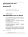
4.1. Introduction .................................................................................................. 51
4.2. The pipeline tasks more fully explained ............................................................. 51
4.2.1. Level 0 to 0.5 .................................................................................... 51
4.2.2. Level 0.5 to 1 .................................................................................... 53
4.2.3. Level 1 to 2 ....................................................................................... 55
4.3. The Status table ............................................................................................ 57
4.4. The Blocktable ............................................................................................. 57
4.5. Converting cube and frame spectra to other formats, to do spectral mathematics ......... 57
4.5.1. A projectedCube ................................................................................. 57
4.5.2. A rebinnedCube ................................................................................. 58
4.5.3. A pacsCube ....................................................................................... 59
4.5.4. A frame ............................................................................................ 59
4.6. Data/observing/instrument issues ...................................................................... 59
4.6.1. Nodding ............................................................................................ 60
4.6.2. Dithering/Rastering ............................................................................. 60
4.6.3. The PSF ............................................................................................ 60
4.6.4. Flatfielding and flux calibration ............................................................. 60
4.6.5. Saturation .......................................................................................... 60
4.6.6. Glitches ............................................................................................ 60
4.6.7. Errors/Noise ....................................................................................... 60
5. In the Beginning is the Pipeline. Photometry ................................................................ 61
5.1. Introduction .................................................................................................. 61
5.2. Retrieving your ObservationContext and setting up .............................................. 62
5.2.1. Scan map AOT .................................................................................. 62
5.2.2. Point Source AOT .............................................................................. 64
5.3. Level 0 to Level 0.5 ...................................................................................... 65
iii
PACS Data Reduction Guide
5.3.1. photFlagBadPixels ..............................................................................
5.3.2. photFlagSaturation ..............................................................................
5.3.3. photConvDigit2Volts ...........................................................................
5.3.4. addUtc ..............................................................................................
5.3.5. photCorrectCrosstalk ...........................................................................
5.3.6. photMMTDeglitching and photWTMMLDeglitching .................................
5.3.7. convertChopper2Angle ........................................................................
5.3.8. photAssignRaDec ...............................................................................
5.3.9. cleanPlateauFrames .............................................................................
5.4. The AOT dependent pipelines .........................................................................
5.5. Point Source AOR .........................................................................................
5.5.1. Level 0.5 to Level 1 ............................................................................
5.5.2. Level 1 to Level 2 ..............................................................................
5.6. Scan Map AOR ............................................................................................
5.6.1. Level 0.5 to Level 1 ............................................................................
5.6.2. Level 1 to Level 2 ..............................................................................
iv
66
66
67
67
67
68
68
69
69
70
70
70
74
76
76
77
Chapter 1. A First Quick Look at your
Data
1.1. Introduction
If you are reading this guide during or in the few months after the Science Demonstration phase
of Herschel then please bear in mind that it is not complete; in particular the links are not active
and the Appendix and some of the later chapters not written or are still being updated. In addition, many issues to do with the pipeline and the data structure are still under consideration
and will change throughout this period. The general documentation on HIPE is also undergoing changes; depending on when you are reading this, the names of other documents referred
to may be different to what is given here: we refer to the Quick Start Guide (QSG) and the
HIPE Owner's Guide (HOG) but under the older organisation these are both in the HowTo
guide (HowTo); we refer to the Data Analysis Guide (DAG) and the Scripting and Data Mining
(SaDM) guide but in the older organisation these are in the Advanced User's Manual (AUM).
...
Welcome to the PACS data reduction guide #. We hope you have got some good data from PACS and
want to get stuck in to working with them. In this guide we will (i) show you how to have a first quick
look at your pipeline reduced data, (ii) explain how data are gathered by PACS and hence how they are
structured, and summarise the pipeline steps, (iii) show you how to go through the pipeline yourself,
(iv) show you how to inspect the products you produce as you proceed through the pipeline, (v) explain
more fully what the pipeline steps are doing, why they are doing it, and what their parameters are,
and (vi) discuss issues that are of concern for particular AOTs (such as rastering) or targets (such as
moving targets) or are still under development.
This guide is aimed at those who are new to HIPE and new to PACS. It will take a while to get
used to HIPE and to reducing PACS data, so allow yourself a lot of patience. Satellite sub-mm data
are complex because the detectors and the observing requirements are. If the data reduction seems
difficult to you it is not because we have made it so, but because it is so. Our aim with this guide is
to teach by doing: we will take you through the pipeline as a tutorial, so you can learn what to do
and how to inspect what you have done. Along the way we will explain the what and the why of the
data reduction. We recommend you run though the pipeline once following this guide, and then if you
want to change some things you can run through it again on your own. This guide is designed to be
read from beginning to end, so read the whole thing before you claim something is not working or
not understandable.
HIPE is the Herschel Interactive data Processing Environment. HIPE is not just for running the
pipeline, it provides an environment in which you can also analyse data using tools provided or by
writing your own scripts. In HIPE you can write scripts to do any type of manipulation, mathematics,
reformatting, analysis, or fitting on your data. Because it uses jython (python, java) it may be unfamiliar to many astronomers, but python and java both are languages that are well worth learning. Note that
while python and java can be used within HIPE, the actual language is (H)DP, that is the (Herschel)
Data Processing language. So some jython-ese will not work and there are additional capabilities that
have been programmed into HIPE that are unique. Scattered throughout this guide are "seed" scripts,
which were written primarily to accompany the pipeline to allow easy plotting and inspection of the
data, but you can also use them to start to learn the scripting language yourself. There is also much
help on DP scripting available from the help page, however, unless you are a good programmer, it is
probably a good idea to first work your way through the pipeline and this PACS data reduction guide,
before starting to script. Doing it the other way around will guarantee much frustration.
There are a number of documents you could read before and along with this one. This may sound
boring, but unless you want to use the pipeline just as a black box you really should read-while-youtry. While this PACS data reduction guide is meant to be complete, it is not stand-alone: we link you
to other documents rather than repeat here what they explain.
1
A First Quick Look at your Data
1) A guide to HIPE itself is provided on the HIPE help page (Help#Contents, from the HIPE menu) in
the HIPE Owners Guide (HOG) and the Quick Start Guide (QSG) (under the older Help organisation
these documents are contained in the HowTo guide). These tells you how to start up and work in HIPE,
how to extract data from the Herschel Science Archive (HSA), and some basics about working with
spectra, cubes and images.
2) The Data Analysis Guide (DAG) tells you about the tools that are provided in HIPE for you to do
your data analysis (everything you do after your pipeline data reduction). (Under the older organisation
this is called the Advanced User's Manual: AUM.)
3) The Scripting and Data Mining guide (SaDM) (or the AUM under the older organisation), also
available from the HIPE help page, contains a lot of information about working in HIPE with arrays,
the DP syntax and working therein, doing mathematics, plotting and displaying. This is recommended
to be read after you have worked your way through the first chapters of this PACS guide: here we
give specific examples of working in HIPE with your data and using the DP language, and there you
can go for the more general instructions.
4) The HIPE help page also has a search capability, in which you can type in the names of tasks or
acronyms that are unfamiliar to you.
5) At least one other document for PACS will be provided (which may not yet be available) on the
HIPE help: the PACS Detailed Pipeline Document (PDPD). This discusses the glorious details of the
pipeline tasks and may include a product description section (i.e. explaining what is what in PACS
products). We strongly suggest you do not read the PDPD until you have read this PACS data reduction
guide first.
6) The HCSS or PACS User's Reference Manual (the PACS URM is the HCSS URM + extra PACS
bits): these contain information about many of the tasks you will use, but be warned that these have
been written by and for internal PACS users and hence may be rather difficult to understand.
7) Another very advanced document is the Developer Reference Manual, which gives you information
about the java classes that underlie the DP system. This will be very difficult to understand at first if
you are not a (java or python) programmer, but hopefully some of the examples provided in this guide
will help you to understand what you read in the API.
1.2. Structure of this guide
In this first chapter we explain how to get your observations from the HSA and look at your Level
2 product, that is data which has already been pipeline-processed. In Chapter 2 we summarise the
data reduction steps from Level 0 (minimally processed) to Level 2 (science quality), and explain
a little about how the data are structured. Chapter 3 takes you through the pipelines for the various
spectrometer AOTs, with some detail about what you are doing at each stage and presenting you with
inspection recipes. The pipeline tasks and inspection recipes are expanded on in Chapter 4 and issues
of concern for particular AOTs or types of targets are discussed. Chapters 5 and 6 are the same as 3 and
4 but for the photometer. Finally, in the Appendix we may include some seed data inspection scripts.
Note that chapters 4,5 and 6 are incomplete (or lacking) and the Appendix has not yet been written.
1.3. A quick-look at your data
Your observations have been performed, now you probably want to know what they look like. This
section will show you how to grab the fully pipeline-processed data and look at them. If you then want
to run the pipeline yourself you will read Chap. 3 and onwards; but it is a good idea to first have a
quick look at your data, to at least see what it is you have be given!
For spectroscopy these fully processed products are cubes, that is data with two spatial axes and one
spectral axis (the PACS spectrometer is an integral field spectrograph). If you are not familiar with
2
A First Quick Look at your Data
looking at cubes we suggest you read up a little on integral field spectroscopy before you start working
on your PACS data, because in this data reduction guide we explain only how to work with PACS
cubes, not all about integral field spectroscopy. For photometry the fully-processed data are a stack
of frames (images/maps).
Start up HIPE. If you followed the installation instructions this should be a matter of simply typing
"hipe" on your command line or clicking on an icon. We recommend that you run HIPE with at least
2GB of memory, more if you can. To increase the memory allocation you can either change it on the
HIPE command line—but the allocation will go back to default next time you start HIPE—or you can
edit one of the "hcss properties files" before starting HIPE. For instructions, see the HOG. (You can
also use the Edit#Preferences menu to change various HIPE properties.) If HIPE runs low on memory
(it has a tracking bar to show memory use) it will freeze and you may have to kill your session, so
don't stint on allocating memory.
When you start up HIPE first go into the Work Bench or the Full Work Bench perspective, by: clicking
on the "Work Bench" icon on the HIPE welcome page; clicking on the small blue (Work Bench) or
green (Full Work Bench) clapperboard icon at the top right of the HIPE GUI; selecting from the menu
at the top left, Window#Show Perspectives. It is in the Console section of your work bench that you
type commands.
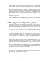
1.3.1. First: get your data and populate your pool
First you need to get hold of your entire dataset and then you need to extract from that the "ObservationContext". There are a number of ways of doing each of these separately and at least two ways of
doing them both together. (Read this section and the next before you try to do anything yourself. And
note that while you may not understand why you are being asked to do all you have to do, it should
become more clear as you go through the later chapters of this guide.)
The instructions for retrieving your data from the HSA and reading them into HIPE or transferring
them to disk are in the QSG, and these instructions we do not repeat here. Essentially you can either
request data as a tarball which you ftp to your own disk and then load into HIPE when you need it, or
you can call on the HSA directly to fetch the data and place it in memory in HIPE. For both methods
you will need to save the data to disk, as a "pool", otherwise next time you run HIPE you will have
to retrieve those in the same way data again. (The ftp method is best if you have many observations
you want to get hold of, direct retrieval best if you are only looking at a few datasets.) Note that there
is usually more than one way to do the same thing in HIPE, so don't worry if you get what appear to
be conflicting instructions when reading different documentation: simply try them out and see which
method you prefer.
A "pool" is simply a collection of data that belong together—your HSA-obtained data, maybe all your
observations of the same object, or all your Level 1 processed products, or everything you worked
on in a single day. The commonality between the products in a pool is yours to decide upon. Inside a
pool will be many FITS files organised in a particular directory structure that allows the links between
related data products to be made. It is the need for these links that is the reason why Herschel data are
held in pools, and is also the reason why Herschel products can sometimes take a while to be extracted
from or into a pool. Because the data in a pool are linked to each other, it is necessary to use the tasks
we provide to inspect, query, and access them. You cannot simply read a single FITS file from a pool
into HIPE and necessarily expect that you can do something with it.
A pool can hold any type of Herschel data product, not only the ObservationContext that you will start
with in your data reduction experience. You can export products that you produce in the course of your
data reduction into pools (more of that later). If you wish to share pools, to send someone processed
data for example, tar up the whole directory and send them that. The pool's directory name must not
be changed or HIPE will not be able to find the data therein.
Note that HIPE expects pools to be located at [/Users/me/].hcss/lstore (i.e. off of your home directory).
lstore is the default supradirectory in which you place all your pools. In Chap. 3/5 we will explain
how to change the default location of /lstore.
3
A First Quick Look at your Data
1.3.2. Next: get the ObservationContext
What you want to look for in your pool/HSA untared directory is the "ObservationContext" (the capitalisation and concating is a jython thing). An ObservationContext is a container of data products that
belong to a specific observation (and ObservationContext is the HIPE class of this container#more
on classes later). It provides the associations between all the products you need to process that single
observation and also includes the results of the automatic pipeline reductions done by the HSA. The
products contained in an ObservationContext include not just the actual astronomical observation (raw
and reduced), but also the data products that were used to process the data in the automatic pipeline,
such as: spacecraft pointing, time synchronisation data, the satellite orbit, the parameters you entered
in HSPOT when you submitted the proposal, and the pipeline calibration tables. The reduced data
contained in the ObservationContext are spectra and spectral cubes or images (spectrometer and photometer respectively); also provided should be a quality assessment of the observation/reductions.
Read the QSG (really...do) for instructions on the most straightforward way to get data from the HSA,
or the <LINK> for a listing of all the methods you can use. Summarising all, and introducing 2 tasks
that are (currently) unique to PACS:
• If you loaded your HSA-requested data directly into the HIPE memory via "Send to External Application" in the HSA view, then you have already the ObservationContext#you have the file that
we call "myobs" below (although its name will not be myobs#look for it in the Variables panel after
you have imported the data and you will see it there listed; if you wish you can change the name
with a right-click on it in the Variables panel).
• If you got your data via ftp from the HSA then you need to import them into HIPE using the "import
Herschel data into HIPE" view (accessed from the HIPE Window menu: see the QSG). This will
extract the ObservationContext from the directory that you untared the data into and put it directly
into a user-chosen pool, let's say a pool called "swimming" (by default it will expect "swimming" to
be a directory already in [HOME]/.hcss/lstore/swimming, so if it does not exist you will first need
to use the PAL to set up "swimming" as a pool). You will then need to get the ObservationContext
from that pool into HIPE in the following way:
myobs=getObservation(1342182002L ,poolName="swimming" ,od=231)
The number specified as the first parameter is the "obsid": this is the observation identifier and is
1342182002 here (this number you should know already, but if not you can hunt for your observation in the HSA and the obsid will be there listed); don't forget the "L" at the end of the number. The
parameter poolName is the name of the pool into which you had placed the ObservationContext
(here that would be "swimming"). The task run with these two parameters will find the ObservationContext with that obsid and in that pool (it is important to specify the obsid, in particular because
more than one obsid can be held in a single pool). You may find that you need to specify also the od
(observing day=231 here—information that should also be listed in the HSA listing of your observation). When you have executed this command, "myobs" will appear in the Variables panel listing.
• If your ObservationContext is in a pool already (e.g. someone sent you an entire pool that they had
already looked at) you get the ObservationContext using the same command getObservation.
• If you got your data via the "Retrieve" button: You use the same method for importing data into
HIPE for that when getting data via ftp. Note: if you used the "Retrieve" button but only on the
Level 2 product, you may not at present be able to use the this interface to get the data (this is being
fixed). Another Note: when I tried this "retrieve" method on an ObservationContext, it was much
slower than the "send to external application" method.
• If you have not already gotten your data from the HSA and put them in to a pool, and if you know
the obsid and don't want to use the GUIs to access the HSA, then with the following command you
can get your data and import them into HIPE:
myobs=getObservation(1342182002L, useHsa=True)
4
A First Quick Look at your Data
For this to work you must have your HSA username and password written in your /.hcss/user.props
file with the following lines:
hcss.ia.pal.pool.hsa.haio.login_usr = your username
hcss.ia.pal.pool.hsa.haio.login_pwd = your password
If you are only now writing these in that file, then you should restart HIPE for it to take effect.
Alternatively you can type directly into your current session the commands:
login_usr = "hcss.ia.pal.pool.hsa.haio.login_usr"
login_pwd = "hcss.ia.pal.pool.hsa.haio.login_pwd"
Configuration.setProperty(login_usr,"xxxxxx")
Configuration.setProperty(login_pwd,"xxxxxx")
We recommend you immediately then save myobs to a pool, because with getObservation you only
load the ObservationContext into HIPE memory, not onto disc.
• If you want to look at what observations are in a pool
allObs = LocalPool("swimming", "/Users/me/.hcss/lstore").allObservations
and then double click on allObs in the Variables panel for a listing.
• You save myobs to a pool in the following way
saveObservation(myobs,poolName="swimming")
where "swimming" is located by default at [HOME]/.hcss/lstore/swimming.
These methods work for an ObservationContext, not for any other type of product. For importing and
exporting other products, see the instructions in Chap. 3/5. The full range of parameters for getObservation and saveObservation are given in Chap 3/5, where we also tell you how to save to a location
on disc other than the default. Right now we want to keep things short and sweet.
Note
You can give you variables#the things on the left of the = sign#any name you like. So
instead of "myobs" you could write "anobs" or "elmioobs".....
Be aware that when you enter od=number, that number must have no leading 0s. 0045 is
not the same number as 45!
1.3.3. How can I work out what is what in the ObservationContext?
One thing that will help you work out what your observation is of and what instrument configuration
you had is to have a copy of the AOR (the Astronomer's Observation Request), which is where the
commanding of the pointing and the instrument configuration would have been taken from. You can
also look at the "meta data" of the ObservationContext. These are like FITS headers, a listing of various
information about a product. Most products will have meta data, although they will not always be
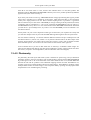
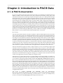
complete. For your ObservationContext, if you click on the ObservationContext itself you will see
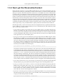
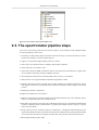
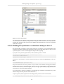
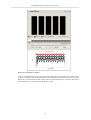
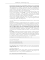
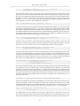
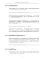
the meta data for it. This is shown in the following screenshot: what you will see if you view your
ObservationContext with the "Observation Viewer". Look for "myobs" in the Variables panel (HIPE
main menu Window#View#Variables). Double clicking on myobs will open a viewer (double click
for the default viewer, right click to get a menu of viewer and other options). The viewer opens in
the Editor panel.
5
A First Quick Look at your Data
Figure 1.1. Meta data
Listed in red are the various individual products that are associated with myobs (more on those in
the next section). The top listing are listed meta data. You can scroll down this list to see everything
listed in there, which includes the parameters commanded in the AOR of your observation: pointing;
repetition factors; observing mode; raster movements; band/wavelength.
If you click now on one of the products listed at the bottom-left ("Data") of the window (e.g. "+level2")
the meta data now listed at the top are those associated with that particular product. There will be less
meta data here than for the ObservationContext (myobs, though in the screenshot it is called"obs"). To
see the myobs meta data again, simply click on "myobs" (which will be at the top of that bottom-left
window, with a folder symbol next to it).
If you have multiple settings in your observation, for example rastering or dithering or cross scans,
then unfortunately at present it is not easy to immediately work out what product is what part of your
observation. This is something we are working hard to improve.
1.3.4. Then: look the Level 2 products
(This section should also be read by people interested only in photometry.)
1.3.4.1. Spectroscopy
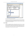
To look at what is in myobs, in your ObservationContext, again open the Observation Viewer on
myobs:
6
A First Quick Look at your Data
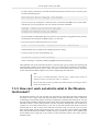
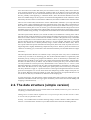
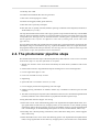
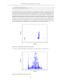
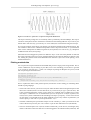
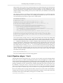
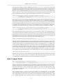
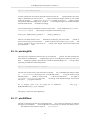
Figure 1.2. Your second glance at an ObservationContext with the Observation Viewer
(A listing in red means that has not yet been loaded into memory, black means it has been loaded
into memory.)
The entries with + next to them can be thought of as directories of data. In each are products that
correspond to the directory name, e.g. quality information are held in "quality". As here we are showing
you how to look at a Level 2 (fully processed) product, you need to look at the "level2" entry. If there
is no "level2" entry there, it means that your observation has not been processed through the automatic
pipeline to that level, and hence there are no cubes or maps for you to look at. In that case you will
need to reduce the data yourself through the pipeline. However, you should still read the rest of this
chapter because it contains useful information that is not repeated in Chap. 3.
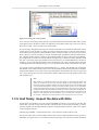
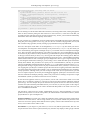
Click on the + next to it "level2" see what lies therein. You will see something like this:
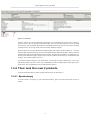
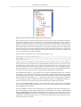
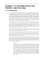
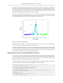
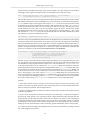
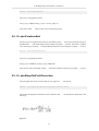
Figure 1.3. A further inspection of your ObservationContext
The screenshot shows you a listing of what is in the Level 2 of your ObservationContext. Listed there
should be HPS3D[PB|PR|RB|RR] (or something similar: it changes faster than I can keep up!). The
7
A First Quick Look at your Data
final "B" or "R" means "blue" or "red", and the "3D" indicates that it is a 3D (cube) product. The
difference between HPS3DPB and HPS3DRB is that they are Level 2 products produced by different
pipeline tasks (more of that in Chap. 3).
If you move your mouse over the e.g. +HPS3DPB a banner will pop up indicating what type of product
(what "class" of product) it is. It should say "ListContext", which means that this is a list of products
(cubes), not a single product on its own. There could be anything from 1 to [a number > 1] products
therein contained. If you click on the +HPS3DPB you will get a listing of all the products (the cubes)
contained in this list, numbered 0..1..2 etc. In our screenshot the HPS3DPB has only one cube in it,
the HPS3DRB has many. Hover over one of the numbers of the HPS3DPB and the banner should tell
you that this is a SpectralSimpleCube; if you hover over the HPS3DRB you will be told that it is a
PacsRebinnedCube.
Exactly what is in your Level 2 depends on what type of observation you requested. It is likely that
you will have multiple cubes if your AOR included dithering/rastering/more than one spectral line.
You will need to read Chap. 3 to find out what the difference between the SpectralSimpleCube and
PacsRebinnedCube is, but for now, suffice it to say that the rebinned cube is the final output of the
pipeline, which takes the 5x5 simple cube as input and "projects" it into a cube of smaller sized but
more abundant spaxels. You can chose to look at either or both of these cubes right now.
In the screenshot above you can see that within the +0 "directory" are datasets called "image" etc.
These are the datasets that make up the cube, these including the "image" (which contains the cube's
flux values), "exposure" and "ImageIndex" (which contains the cube's wavelengths).
1.3.4.2. Photometry
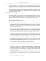
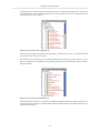
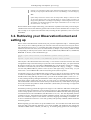
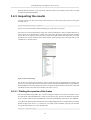
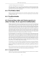
For photometry the same layout and similar syntax is found as for spectroscopy, and you should see
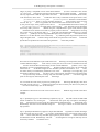
something similar to the next screenshot. This includes products with the names HPP[N|M]MAP[B|
R], where again a "B" or "R" as the final letter in the name stands for blue or red, and the difference
between the "M" and "N" products is that a different mapping scheme was used. The HPPxxxx are,
as before, ListContexts and the products therein are SimpleImages. These HPPxxxx products contain
multiple dataset within: the actual image, a noise map and a history reporting on what pipeline tasks
and parameters were used during the processing.
8
A First Quick Look at your Data
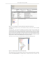
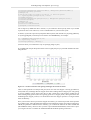
Figure 1.4. ObservationContext layout for photometry
In fact, whatever is (are) listed there in the Level 2 box is (are) what you want to look at, the differences
between products there listed being the band and the type of map/cube that was made. More than one
product will be listed, because more than one band and more than one type of map will be provided,
and repetitions may be held separately and/or combined into one. In Chap. 2 and onwards we explain
more about what these various products are.
1.3.4.3. Both
To now view your product(s) (the maps or cubes) you need to click on the +0 (or +1...) (not the
datasets) next to the HPxxxx entry you are first interested in. This will give you access to the various
viewers for your product. A double-click gives you the default viewer, a right-click gives you a viewer
menu. The default viewer for spectroscopy should be the CubeAnalysisToolBox (because the Level 2
product is a cube). The toolbox will open in the window to the right of the listing (where the spectrum
you can just about see in the screenshot is), and/or in a new tab. For photometry the default viewer is
the Standard Image Viewer (as shown in the previous screenshot).
9
A First Quick Look at your Data
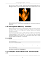
Figure 1.5. Viewing your Level 2 product
Note: as we are still working on the pipeline it is possible that the here-mentioned GUIs will not work
on the data you have. Whatever viewers are offered for your product are the only viewers you can use.
However, in Chap. 4 and 5 we offer some workarounds.
For spectroscopy and photometry both you could also export the Level 2 product to FITS files and use
a FITS viewer to look at them. To do this you need to extract the maps or cube out of the ObservationContext first. We postpone a full explanation of how to do this to Chap. 3/5 but in case you want to
know right now: you can click-drag a +0 to the Variables panel, and that will selected out that particular cube/map product. When it appears in the Variable panel it will have a name like "newVariable".
If you right-click on it there, you will be offered the opportunity to "Send to" FITS (remember to add
the ".fits" to the name, and it is by default saved to the directory you started HIPE from), and also to
rename it. As you click-drag the product to the Variable panel you will see echoed to the Console the
command that does this self-same thing (so you can do this yourself on the command line next time).
If you want to inspect separately the individual datasets, e.g. "image", then double click on them for
their default viewer which will also open in a new tab (and which will not be the CubeAnalysisToolBox
because these datasets are not cubes, they are the information that are held in the cube), or right click
for a viewer listing. But at present viewing these datasets rather than the entire product will be less
than useful for you.
Note
Data products are of different classes. The class types are indicated in this guide with
italics, for example the Level 2 cube "mycube" should be a SpectrumSimpleCube. You
can tell what class a product has either by hovering the mouse over it in the Variables panel
to see the information banner; clicking on it in the Variables panel to see an information
listing in the Outline panel,;or typing >print mycube.class in the Console panel. The class
of a product defines what information are held in it and their organisation, and depends on
what level of the pipeline the product has been taken to. Tasks, functions and GUIs are all
written to work on specific classes of products, so if you cannot use a particular viewer,
for example, it means the class of the product you are trying to use it on is incorrect.
1.3.5. And finally: inspect the data with GUIs
In this section we introduce you to the viewers that HIPE provides for you to look at your data. We
assume that you want to only look at the data, and maybe have a play around with what is in them;
the main emphasis of this Data Reduction Guide is the pipeline data reduction, which is the subject
of all subsequent chapters.
The help page of HIPE—in particular the DAG—is the reference for data analysis tools.
For spectral cubes, what you will probably want to look at is the spatial distribution of your spectra, to
find where your point source is or to make an emission line map. You will want to look at the spectra
10
A First Quick Look at your Data
from individual spaxels, to access the quality of your data, and maybe add together spaxels to get a
spectrum of everything in your field of view (be it a point or an extended source). For photometry you
will probably want to look at the maps of different scans, to see how well the map construction has
been done, what the background looks like and whether the maps from different scans look the same.
For some of the GUIs you need to extract out of the ObservationContext the cube or map. You do this
with the click-drag we explained above, for the cube we assume that you have called that new product
"mycube" and for the map, "mymap".
1.3.5.1. Spectroscopy
Before beginning we would like to point out that currently, while we are still in the first year of Herschel, the tools for doing spectral manipulation are still under development, and at the time of writing
they do not all work directly on PACS cubes. Hence I warn you now that this part of working with
PACS spectroscopy data will be rather frustrating. Some workarounds are provided in Chap. 4.
Here we will introduce you to the various GUIs that can be used to inspect your PACS cube of class
SpectrumSimpleCube. There are other ways you can inspect (and later manipulate) the data, but for a
first quick-look we recommend you use the GUIs.
• # The SpectrumExplorer. This is a spectral visualisation tool for sets of 1d spectra and at some
point also for your Level 2 SpectralSimpleCube. It allows for an inspection and comparison of
spectra from individual spaxels. It is probably easier to use than the CubeAnalysisToolBox if you
are interested in only looking at individual spectra. The DAG provides a guide to the use of the
SpectrumExplorer, and it is called up with a right-mouse selection on mycube in the Variables panel.
It may at present not work on cubes.
• # The CubeAnalysisToolBox. This allows you to inspect your cube spatially and spectrally at the
same time. It will allow for some analyses#you can make line flux maps, position-velocity diagrams
and maps, extract out spectral or spatial regions, and do some line fitting. The DAG includes a guide
to this GUI, and it is called up with a right-mouse selection on mycube in the Variables panel. It
currently works on the SpectralSimpleCubes and the PacsRebinnedCubes if the WCS is valid.
• # The SFTool. The SpectrumFitterTool will allow you to fit and do mathematics on your spectra.
To access the SFTool, click-highlight mycube in the Variables panel; go to the Task panel at the
top-right of the Full Workbench; and double click on Applicable. All applicable tasks will be listed,
this will include certain mathematical functions and the SFTool. The DAG explains the use of this
tool, which unfortunately at the time of writing does not work directly on PACS cubes.
• # The ExplFitter. The line fitting tool (similar to the SFTool). This is also to be found in the Tasks
panel and details of use are in the DAG. It also allows for spectral line and continuum fitting. It may
also at present not work directly on PACS cubes.
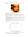
• You can image single or multiple wavelength slices of your cube with Display.
Display(mycube.flux(1000:1100,:,:],depthAxis=0)
will display as a 2D image 100 wavelength bins (1000:1100, and you can scroll through the layers
in the display) for all spaxels of your cube (the :,: part of the command). Don't try to display all the
wavelength layers: you may use up all your memory and HIPE will freeze! Unfortunately you need
to specify the array position (1000 to 1100 here), not the actual wavelengths. To figure out what
array positions corresponds to which wavelengths you need to inspect your cube, and for now the
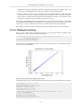
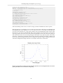
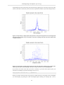
most straightforward way to do this is to plot the wavelengths against array position:
PlotXY(mycube.getWave())
plots the wavelengths on the Y-axis and array position on the X-axis. We explain the syntax of this
command in Chap. 3.
• You can plot single spaxels with the command
11
A First Quick Look at your Data
PlotXY(mycube.getWave(),mycube.getFlux(12,11))
where 12,11 is the spaxel you are plotting (the dimensions can be found with > print
mycube.dimensions, where the final 2 are the spatial dimensions and the first is the spectral dimension).
1.3.5.2. Photometry
There are fewer separate GUIs for image viewing and analysis than there are for spectra, so there is
less for you to learn about! There is one GUI which provides a first look and quick quality assessment
of the data: the Standard Image Viewer (SIV). You call this either with a right-click on mymap in
the Variables panel or the +0 entry of the ObservationContext, as explained before. If you want to do
image analysis then HIPE provides many separate tasks you can run, to do contouring, overlaying,
photometry, mathematics, etc. You access these tasks by click-highlighting mymap in the Variables
panel, and then looking to see what "Applicable tasks" are listed in the Tasks panel of HIPE (one of
the "viewers" you can access from the main HIPE window menu). The instructions for using these
tasks are in the DAG.
12
Chapter 2. Introduction to PACS Data
2.1. A PACS observation
If you are not familiar with how PACS observations work we recommend you read the Observer's
Manual (<LINK>). PACS observations involve the synchronised movements of many parts of the
instrument for the purpose of exploring the spatial and spectral space your AOR specified. During a
PACS observation you can have: chopper movements between two mirror positions (to account for
the rapidly varying telescope background); nodding of the telescope between two fields (to remove
the astronomical "sky" background); moving over many fields to make a bigger map; grating movements to sample the wavelength domain (for spectroscopy). All of these movements are tightly synchronised, so that at each field-of-view of each nod, the right (same) number of chops and right (same)
wavelength range and sampling are included, and the nods are positioned and timed to fit in correctly
with movements between consecutive (mapping) fields-of-view. The grating moves in discrete steps,
usually down the wavelength range and back up again (and maybe more than once), during which the
chopper will be chopping. Thus, moving along the time axis you are not just gathering more and more
photons, but you will be looking at different sky positions, different wavelengths, and different focal
plane positions. It is this instrument dance that the pipeline has to account for.
Spectroscopy:
The PACS spectrometer detectors are photo-conductors. When far-infrared photons fall onto the detector crystal, charge carriers are released that enable an electric current to flow through the detector.
These currents are integrated over a capacitance. The more flux that falls onto the detector, the faster
the voltage over this capacitance increases, and the larger the signal value will be. It is this voltage increase that is measured in the PACS detector electronics. The voltage over the capacitance is read out
at 256Hz. Typically, the detector capacitance is discharged every 0.125 or 0.25 seconds#the detector
is read out non-destructively (usually 32 or 64 times) before a destructive readout is performed, i.e. the
voltage across it is reset to a reference value every 0.125 or 0.25 seconds. The non-destructive reading
out is accumulative, that is the signal you read for readout at time T(2) is the value of the signal of
readout at time T(1) plus the extra that is due to the light that fell on the detector since time T(1).
The raw PACS detector signals are ramps ("ramp"#"incline") of 32 or 64 increasing voltages. This
information cannot be downlinked in its raw volume (which is huge), except for 1 pixel which is fully
read out for data-checking purposes (by the PACS instrument team); therefore the instrument reduces
the data on-board. For short ramps (32 samples) a slope fitting is done, and per pixel one number
(the value of the slope) per integration ramp is downlinked and visible at Level 0. For long ramps (64
samples) the on-board software averages the voltages per 16 samples. In that case the Level 0 data
consists of averaged ramps with four numbers per integration ramp.
The easiest way to check which of the two on-board reductions has been applied to your data is to
check the Level 0 data (in the same way as explained in Chap. 1 for looking at what is in Level 2). If
you see in the Level 0 listing product branches with the name HPSFITB or HPSFITR (Herschel-PacsSpectroscopy-FITted-Blue, Herschel-Pacs-Spectroscopy-FITted-Red) then on-board slope fitting was
done, and you start the pipeline processing from these Frames "class" products. If you see products
with the name HPSAVGB or HPSAVGR (Herschel-PacS-AVeraGed-Blue detector, Herschel-PacsSpectroscopy-AVeraGed-Red detector) then the integration ramps were averaged on-board and you
start the pipeline processing from these averaged Ramps class products. The dimensions of a HPSFITR product will be something like 18,25,980 (18x25 pixels, each with 980 readouts along the time
dimension; later this time dimension is turned into the wavelength dimension). The dimensions of
the equivalent HPSAVGR product will be 18,25,980,4 (each of the 980 individual ramps contain 4
averaged readout values).
The Level 2 products HPS3DRR and HPS3DPR stand for Herschel-PacsSpectroscopy-3Dimensional-Rebinned_cube -Red (which is of class PacsRebinnedCube), and Herschel-Pacs-Spectroscopy-3Dimensional-Simple_cube-Red (which is of class SpectralSimpleCube).
At Level 1 we also have the HPS3D[B|R], these being of class PacsCube.
13
Introduction to PACS Data
Your observation will contain data from your astronomical source, auxiliary data to allow the telescope pointing and timings to be calibrated, calibration data so the detector response and dark can
be corrected, and more. In your astronomical dataset(s) there will be data not just from your target
but also, probably in the beginning, a "calibration block", where the internal calibration sources are
observed. Gradual changes to the response of instrument and degradations of the calibrators will be
followed by the PACS team over the lifetime of Herschel, and will be included in the calibration data.
There is also a Status table, and later there will be a BlockTable, attached to your ramp and frame
products, these contain information about the instrument status of the data and its organisation (in
time). These are added to (and changed) as the pipeline proceeds. If you double click on e.g. a Level 1
frame in the Variables panel to view its contents, you will see the Status table there. Right click to select
the Dataset Viewer (or the Table plotter, although this cannot plot all the entries of the Status), and you
will see a tabular listing. In Chap. 4 we explain the most useful entries of the Status and Block tables.
The PACS spectrometer detectors (one red and one blue) are of dimensions 18 along the Y and 25
along the X. Each of the 25 columns are a single spaxel, and collectively these have an on-sky arrangement of 5x5. These columns are referred to as modules: a module is the physical entity to which the
column corresponds to in the instrument. Each column contains 18 pixels (hence 18 rows), although
the first and last hold no astronomical data (the first is an open channel, which has no associated
detector unit, and the last is a dummy channel, being a resistor instead of a detector unit). The 16
active pixels collect the spectral information for their spaxel, where each of the 16 pixels sees a wavelength range that is slightly shifted along compared to the previous. These 16 pixels are also known as
"detectors"#confusing, yes, but the name comes from the fact that they are each little detectors of light.
Photometry:
The PACS photometer detectors are bolometer arrays. Each pixel of the array can be considered as
a little cavity in which sits an absorbing grid. The incident infrared radiation is registered by each
bolometer pixel by causing a tiny temperature difference, which is measured by a thermometer implanted on the grid. What we call "signal" is the voltage measured at this thermometer. The blue channel offers two filters, 60–85 µm and 85–130 µm and has a 32x64 pixel array. The red channel has a
130–210 µm filter has a 16x32 pixel array. Both channels cover a field-of-view of ~1.75'x3.5', with
full beam-sampling in each band. The two short wavelength bands are selected by two filters via a
filter wheel. The field-of-view is nearly filled by the square pixels, however the arrays are made of
sub-arrays which have a gap of ~1 pixel in between. For the long wavelength end 2 matrices of 16x16
pixels are tiled together. For science observations the multiplexing readout samples each pixel at a
rate of 40 Hz. Because of the large number of pixels, data compression is required and hence we do
not see the raw data; they are binned to an effective 10 Hz sampling rate.
As with spectroscopy, the observations contain auxiliary data such as telescope pointing, time, and
calibration information beside the target signal. Photometry observations also include nodding and
chopping, a calibration block, ....................
2.2. The data structure (simple version)
The structure of PACS data are given in better detail in the PDPD, but here we give a overview of
everything you need to know for now.
Although the screenshots and the emphasis here is on spectroscopic data, the data structure is more
or less the same for photometric data.
In Chap. 1 we included some screenshots showing listings of what is held in a PACS ObservationContext. A screenshot of the structure of your ObservationContext will look something like this:
14
Introduction to PACS Data
Figure 2.1. The contents of an ObservationContext for spectroscopy
This screenshot (and you could also look again at those of Chap. 1) shows that within an ObservationContext (called "myobs" here) you find layers of products with names such as level0, auxiliary,
calibration...Within the level0/1/2 "directories" you can see products called HPSxxx (spectrometer) or
HPPxxx (photometer): among these are the products that you will work on, as they contain the actual
astronomical observations. The other directories (e.g. auxiliary and calibration) are extra information
which are necessary for the data reduction but which you do not need to access directly yourself. The
same click methods as previously mentioned can be used to inspect these products (i.e. double-click
to view, right-click for viewing menu listing).
On the Console command line you can print-list these products, e.g.,
print myobs.calibration.spectrometer
print myobs
print myobs.level0
where the first line will produce a listing similar to the next screenshot, the second line produces a
listing of the entries in the meta data (a sort of FITS header) and the "directories" you can see in the
screenshot above, and the third line shows what Level 0 products there are in your ObservationContext. Be warned, however, that this type of syntax will only take you so far: for example to "print"
further something in Level 0 (e.g. HPSAVGB) you cannot type "print myobs.level0.HPSAVGB. We
recommend, in any case, that you stick to the GUI listings rather than the command line.
In the HPSAVGB "directory" (for photometry this would be called HPPAVGB) in the screenshot
above there is only 1 product (0), and in there are the datasets of Status, Signal, and a listing of Masks
(in the beginning there will only be one mask listed). It may be that there is more than one HPSAVGB
product present (referred to then as 0 1 2 3...), and if so you will later need to extract these out separately
to run through the pipeline. What has just been said applies equally to an HPSFITB/R "directory",
which you will have if your data are the fit ramps instead of the averaged ramps products.
There may also HPSRAWB/R "directories", these products being the raw ramps that are downlinked
for 1 pixel and used for calibration purposes (i.e. not by you). The organisation therein is different
than the HPSFIT/AVG products.
All the other HPSxxxx entries in the screenshot above are additional products that contain data necessary for data reduction or data checking. Important for the pipeline are the products called HPSDMCR/B (or HPPDMCR/B), which are the DecMec data (more on this later). Not important for you are
the HPS[HK|GENHK|ENG], which are "housekeeping" and engineering data, information about the
temperatures, instrument settings, status etc. of the satellite and of PACS. These information are for
instrument scientists to interpret.
15
Introduction to PACS Data
A calibration tree, containing all the information necessary to calibrate your observation, comes with
your data and also with your HIPE installation (more on that later). If you click on "calibration" from
the screenshot above you will see:
Figure 2.2. The contents of the calibration tree
These all are the calibration products that were used to produce the Level 0.5, 1 and 2 products that
are all part of your ObservationContext.
The auxiliary tree, shown below, also contains products that are necessary for the reduction of your
data, for example the obit ephemeris and pointing products. These are information that are mainly
about the satellite.
Figure 2.3. The contents of the auxiliary tree
The log and quality listings are: a log of the processing that produced that level's data (even for Level
0 there has been processing to convert the data from raw satellite format to an ObservationContext);
and quality information.
16
Introduction to PACS Data
Figure 2.4. The contents of the log and quality trees
2.3. The spectrometer pipeline steps
Level 0 to 0.5 processing is the same for all AOTs (points 1 to 8) and many of the subsequent tasks
are also performed for most AOTs.
1. If working on Ramps data, flag for saturation. Then fit the slopes to convert the data to a Frames
product. If working on a Frames product skip to 2
2. Signal is converted from digits/readout_interval to Volts/s
3. Status entry for calibration blocks is added to; Status table is updated
4. Spacecraft time is converted to UTC
5. Spacecraft pointing is added to the Status table for the central pixel of the detector; chopper units
are converted to sky angle; pointing is added to all pixels
6. Wavelengths for each pixel are calculated; Herschel's velocity is corrected for
7. Data "blocks" are recognised and the information organised in a table
8. Masking. Bad pixels will have already been masked. Masking for readouts taken during grating
and chopper movements is performed, and for saturation if the data reduction began on a Frames
product
9. Masking for glitches is performed
10.Signal non-linearities are corrected for
11.Signal is converted to a level that would be if the instrument had been set to the minimum capacitance (no change made if that was already the case)
12.The dark current and pixel responses (their individual sensitivities) are calculated using differential
(internal) calibration source measurements to populate the absolute response arrays; a response
drift is then calculated
13.Chop-nod AOT: the up- and down-chops are combined (i.e. a background+dark subtraction); the
signal is divided by the relative spectral response function and then pixel responses (and their drift)
are corrected for; the nods are averaged, such that each nod-cycle (not each nod) becomes one
14.Wavelength-switching AOT: TBD
17
Introduction to PACS Data
15.Off-map AOT: TBD
16.Calibrated 5x5xlambda data cubes are generated
17.The cube's wavelength grid is created
18.Outliers are flagged (another glitch detection)
19.The data cube is spectrally resampled
20.The data cube is spatially rebinned, different pointings combined and resampled (mosaicked) or
3D drizzled (not yet ready)
The steps described here follow those in the "ipipe" pipeline scripts. Within the directory with the HIPE
software, these are hopefully located in /scripts/pacs/toolboxes/spg/ipipe. The name of the ipipe script
corresponds to the AOT type. Bear in mind that this data reduction guide is updated less frequently
that the pipeline tasks, so if there are differences in the order of running tasks, use the order in the
ipipe directory.
For large datasets the data will probably have been sliced, that is organised in distinct and separate, but
linked parts using an "astronomical" logic (e.g. separate the different rasters of a single observation;
keep together all data of the same spectral line). Once this logic has been worked out and incorporated
in the pipeline scripts, that information will be included here.
2.4. The photometer pipeline steps
We summarise here the basic steps of the PACS photometry data reduction. Level 0 to 0.5 is the same
for all AOTs (steps 1 to 10). This information is out of date.
1. Identify the structure of the observation and identify the main blocks (calibration and science
blocks)
2. Perform data cosmetics: flag bad/saturated pixels and flag/correct cross talk and glitches
3. Convert signal from digits to volts
4. Correct for crosstalk Currently on hold
5. Deglitching
6. Spacecraft time is converted to UTC Not yet ready
7. Covert chopper position from engineering units into angle
8. Satellite pointing information are added to frames (sky coordinates of reference pixel for each
readout)
9. The dark current and pixel responses (their individual sensitivities) are calculated using differential
(internal) calibration source measurements to populate the absolute response arrays
10.Flag data taken while the chopper was moving
11.Point Source AOT: check what dithering pattern was implemented and update Status table; average signals taken at each and every chopper position, if more than one in each; add the pointing
information; subtract the nod positions (per nod cycle and dither position); average the differential
nod A and B images; do the flatfielding and response correction; combine dithers; make a map
12.Scan Map AOT: add the pointing information; remove data taken during slews; run the highpass
filter; make a map
13.Small Extended source AOT: check what dithering pattern was implemented and update Status
table; average signals taken at each and every chopper position, if more than one in each; add the
18
Introduction to PACS Data
pointing information; subtract the nod positions (per nod cycle and dither position); average the
differential nod A and B images; do the flatfielding and response correction; another adding of
pointing information; remove data taken during slews; make a map
The steps described here follow those in the "ipipe" pipeline scripts. Within the directory with the HIPE
software, these are hopefully located in /scripts/pacs/toolboxes/spg/ipipe. The name of the ipipe script
corresponds to the AOT type. Bear in mind that this data reduction guide is updated less frequently
that the pipeline tasks, so if there are differences in the order of running tasks, use the order in the
ipipe directory.
For large datasets the data will probably have been sliced, that is organised in distinct and separate, but
linked parts using an "astronomical" logic (e.g. separate the different rasters of a single observation;
keep together all data of the same spectral line). Once this logic has been worked out and incorporated
in the pipeline scripts, that information will be included here.
2.5. The Levels
There is a Herschel-wide convention on the processing levels of its instruments. The different levels
reflect how much of the pipeline has been run to create the data and the amount of additional information that has been attached to them.
• Level 0 data:
Level 0 is a complete set of minimally processed data. After Level 0 data generation (done by the
HSC) there is no connection to the database from which the raw data were extracted (this database
is not available to the general user). Therefore the Level 0 data contain all the information required.
• Science Data
Science data are organised in user-friendly classes. The Ramps class contain (i) raw channel data
(but usually only for a certain number of detector pixels, as these data are huge) (ii) averaged
channel data, for all pixels; and the Frames class, for which on-board fitting of the slopes of the
raw ramps has already been done.
• Auxiliary data
Auxiliary data for the time-span covered by the Level 0 data, such as the spacecraft pointing
(attitude history, which however is only available after Level 0.5), the time correlation, selected
spacecraft housekeeping, etc. The information are partly held as status entries attached to the
basic science classes (Ramp and Frame) and the rest are available as separate products (e.g. the
"pointing product") which you can access.
• Calibration data
This is the data that is used to calibrate the observations. A calibration dataset is included at Level
0, however calibration data is also provided with your HIPE installation, and generally it is the
HIPE calibration dataset you should use when you process your data through the pipeline.
• Quality data
Quality control information, including (or maybe only) messages produced by the processes that
produced the Level 0 data, or messages from the pipeline processing that produces later levels.
• Level 0.5 data:
Processing until Level 0.5 is AOT independent. These data are also present with what you got from
the HSA. At this level additional information has been added to the Frames science products (masks
for saturation and bad pixels, RA and Dec, the BlockTable,...) and basic unit conversions have been
applied (digital values to volts, chopper position to sky angle). For the spectrometer, during Level
0.5 production the Ramps are turned in to Frames.
19
Introduction to PACS Data
• Level 1 data:
Level 1 data generation is AOT dependent (although there will be much overlap between the AOTs).
Level 1 data are also available for selection from your pool, having been processed automatically
at the HSA. Data processing at this level is concerned with cleaning and calibrating, and as the end
the data are converted to a basic spectrometer cube (the 16x25 useful pixels have been converted
to 5x5 spaxels, each holding 16 individual spectra).
• Level 2 data:
Going from Level 1 to Level 2 the spectrometer cube is spectrally and spatially rebinned. At this
level scientific analysis can be performed. Level 2 work is highly AOT dependent.
• Level 3 data:
This is simply a level where the scientific analysis has been done by the data users (e.g. spectral
cubes converted to velocity maps, source catalogues), and it is hoped that users will import these
products back into the HSA.
20
Chapter 3. In the Beginning is the
Pipeline. Spectroscopy
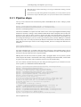
3.1. Introduction
The main purpose of this chapter is to tutor users in running the PACS spectroscopy pipeline. Previously we showed you how to extract and look at the Level 2 fully pipeline-processed data; if you are
now reading this chapter we assume you wish to reprocess the data and check the intermediate stages.
Later chapters of this guide will explain in more detail the individual tasks and how you can "intervene" to change the pipeline defaults; but first you need to become comfortable with working with the
data reduction tasks. To this end the sections here are divided into (i) a listing of the task steps with
brief explanations and (ii) demonstrations for viewing the data just processed: plotting, displaying etc.
More information on inspecting data, on the pipeline, and on particular issues with PACS data are in
Chap. 4. However, we recommend you read through this chapter first, to learn at least how to run the
pipeline and what sort of things you need to do to check the output.
The PACS pipeline can be run in one of two ways: the scripts in the ipipe directory (hopefully in
your installation these are in /scripts/pacs/toolboxes/spg/ipipe and the one you want corresponds to
the AOT name of your AOR, e.g. pacschopnodstarframesIA.py for a pipeline starting from a Level 0
Frames product, or pacschopnodstarrampsIA.py if starting with a Ramps product) can be run in one
go, for example you can load it into the Editor panel and run it (see the note below). Or, you can run the
pipeline as a long series of individual tasks, one by one. If you want to inspect intermediate products
we recommend this method, and it is what is followed here.
We will first take you through the pipeline for a chop-nod observation, then other AOTs will the be
discussed; so if you are working with data from one of these other AOTs we recommend you still read
this entire chapter. At present only chop-nod is discussed.
A suggestion before you begin: the pipeline runs as a series of commands, and as you gain experience
you may want to add in extra tasks, construct your own plotting mini-scripts, write if loops and note
down what it is you did to the data. Rather than running the tasks on the command line of the Console
(and having to retype them the next time you reduce your data), we suggest you write your commands
in a jython text file and run your tasks via this script.
The pipeline steps we outline here are also available in the ipipe scripts (one per AOT). These can be
found in the directory where you installed the HIPE software, hopefully in /scripts/pacs/toolboxes/spg/
ipipe. We suggest you copy the relevant file and open it in HIPE. You can then follow this manual and
that ipipe script at the same time, editing as you go along (and please excuse any differences between
the ipipe script and this guide, but they will not always be updated at the same time: generally the
ipipe scripts should be updated first).
Note
How to create and run a script in HIPE. From the HIPE menu and while in the Full/
Work Bench perspective select File#New#Jython script. This will open a blank page in
the Editor. You can write commands in here (remember at some point to save it...if HIPE
has to be killed you will lose everything you have not saved). As you are doing so you
will see at the top of the HIPE GUI some green arrows (run, run all, line-by-line). Pressing
these will cause lines of your script to run. Pressing the big green arrow will execute the
current line (indicated with a small dark blue arrow on the left-side frame of the script).
If you highlight a block of text the green arrow will cause all the highlighted lines to run.
The double green arrow runs the entire file. The red square can be used to (eventually)
stop commands running. If a command in your script causes an error, the error message is
reported in the Console (and probably also spewed out in the xterm, if you started HIPE
from an xterm) and the guilty line is highlighted in red in your script. A full history of
commands is found in History, available underneath Console for the Full Work Bench
perspective.
21
In the Beginning is the Pipeline. Spectroscopy
Spacing is very important in jython scripts, both missing and present spaces. Indentation is
necessary in loops. Spaces after the end of a line of >if (something):< can mess things up.
Note
Syntax: Ramps and Frames are the "class" of a data product. "Ramp" or "frame" are what
we use in this guide to refer to any particular Ramps or Frames product. A Frame is an
image, for the photometer it is an image corresponding to 1/40s of integration time, for the
spectrometer it is and image made up of the slopes of all detectors over one "ramp" (over
one reset interval—see Chap. 2).
Please read this whole chapter before doing your reductions. Explanations for what you are doing are
included in the sections that detail the pipeline tasks and the sections that detail how to inspect your
data. In Chap. 4 we explain more about the tasks, including all their parameters, here we run with
the defaults.
3.2. Retrieving your ObservationContext and
setting up
How to retrieve the Observation Context from your pool was explained in Chap. 1. Continuing from
there: since you are re-reducing the data you will want to this time start from Level 0 (if you want to
start instead from Level 0.5 or 1, you follow these same instructions but you will start your pipeline
reductions from this later level). You can selected either (i) Ramps or (ii) Frames products to work
on, depending on which you have; these will be called (i) HPSAVGR, HPSAVGB or (ii) HPSFITR,
HPSFITB. To do this, on the command line type:
myramp = myobs.level["level0"].refs["HPSAVGB"].product.refs[0].product
# or
myframe = myobs.level["level0"].refs["HPSFITB"].product.refs[0].product
where myobs is the ObservationContext from Chap. 1. This extracts out from Level 0 the first of the
averaged blue ramps or the blue fit ramps. If you want to start with the red ramps, you replace the final
B with an R. If there is only one product of HPSXXXX then you still need to specify the ".refs[0]",
and if there is more than one you can select out the subsequent with ".refs[1]", ".refs[2]",...... To find
out how many HPSAVGBs are present at Level 0, have a look again at Fig. 3 from Chap. 1; if you
click on the + next to HPSAVGB it will list all (starting from 0) that are present.
An alternative way to get your HPSAVGB..ref[x] product is to click on myobs in the Variables panel
to send it to the Editor panel, click on +level0, then on +HPSAVGB to see the entries 0, 1, 2... You
should be able to drag and drop whichever entry you want to the Variables panel (i.e. the 0 or 1 or...
is what you drag and drop; although I found that in order to drag out the product rather than the entire
observation context, I had to first click on the +0, to turn it into a -0, and then drag and drop the -0).
The command that is echoed to the Console when you do this will be very similar to the one you typed
above, only now the new product is called "newProduct" (which name you can change via a right click
on it in the Variables panel).
PACS data processing proceeds through various stages: Level 0 data have had almost nothing done
to them and is where we begin here. Level 0.5 data processing is AOT-independent, the ramps are fit
to turn a Ramps product in to a Frames one, and information is added to the data (telescope pointing
is translated into RA, Dec and added in, bad data masks are set, etc.). The AOT-dependent part then
continues to Level 1, from which level scientific-grade data is found. At Level 1 the wavelengths will
have been calibrated, response of the detector corrected, chopping and nodding accounted for, etc.
At Level 2 the data are turned in to a 5x5 cube, spatially and spectrally rebinned, and that marks the
end of the pipeline.
Before beginning you will need to set up the calibration tree. You can either chose that which came
with your data or that which is attached to your version of HIPE. The calibration tree contains the
information HIPE needs to calibrate your data, e.g. to translate grating position into wavelength, to
22
In the Beginning is the Pipeline. Spectroscopy
correct for the spectral response of the pixels, to determine the limits above which flags for instrument
movements are set. As long as your HIPE is recent then the caltree that comes with it will be the most
recent, and thus most correct, calibration tree. If you wish to recreate the pipeline processed products
as done at the HSC you will need to use the calibration tree there used, i.e. that which comes with
the data (and which is shown in Fig. 2 of Chap. 1). We recommend you use the calibration tree that
comes with HIPE. Structurally, the two are the same, but the information may be different (more, or
less, up-to-date).
# from your data
mycaltree=myobs.calibration
# or from HIPE recommended
mycaltree=getCalTree("FM")
# where FM stands for flight model and is anyway the default
It is necessary to extract a few other products in order for the pipeline processing steps to be carried
out. These are the dmcHead, the pointing product, and the orbit ephemeris. You can get these with
pp=myobs.auxiliary.pointing
dmcB=myobs.level["level0"].refs["HPSDMCB"].product.refs[0].product
dmcR=myobs.level["level0"].refs["HPSDMCR"].product.refs[0].product
orbitephem = myobs.auxiliary.orbitEphemeris
timeCorr=myobs.auxiliary.timeCorrelation
The pointing product is used to calculate the pointing of PACS during your observation, the dmcB/R,
or the products called HPSDMCB and HPSDMCR, contain the position and status of the PACS mechanisms and detectors sampled at high frequency. The orbit ephemeris is used to correct for the movements of Herschel during your observation, and the time correlation product is used by the time conversion tasks. If the time correlation and orbit ephemeris products are not present, don't worry, you
can run the pipeline for now without them.
Note: It is possible that there will be more than one HPSDMCR/B layer (to check double-click on
myobs in the Variables to send to the Editor; click on Level 0 and then on HPSDMCR/B; if only 0 is
there, there is only 1 layer). This is unlikely, but (especially during SD phase) it is possible. At present
the only way to know which one you want to extract is to look at the "FINETIME" status column, this
being the time stamp (in microseconds). If you print and compare the first and last timestamp for your
frame or ramp and for the dmcHead you should be able to figure out which dmcHead you need. You
can do this with the following commands:
# print the first and last time stamp of your frame/ramp
# (the syntax is the same for both)
print myframe.getStatus("FINETIME").data[0],myframe.getStatus("FINETIME").data[-1]
# then print the same for the layers of the DMCheader
# for the first layer, for the blue one
dmcB=myobs.level["level0"].refs["HPSDMCB"].product.refs[0].product
print dmcB["DmcHeader"]["FINETIME"].data[0],dmcB["DmcHeader"]["FINETIME"].data[-1]
# then do the same for the next layer,
dmcB=myobs.level["level0"].refs["HPSDMCB"].product.refs[1].product
print dmcB["DmcHeader"]["FINETIME"].data[0],dmcB["DmcHeader"]["FINETIME"].data[-1]
# etc
Then compare the results and see which dmcHead covers the time range of your data (they don't have
to match exactly, they just need to cover the same time range).
3.3. Level 0 to 0.5
First we list the pipeline steps, then we tell you how to inspect the products just created. More information about the tasks will be provided in Chap. 4.
Tip
As you run tasks in HIPE you will see a small rotating circle at the bottom right of the HIPE
GUI indicating that "processing is occurring". While this is running you cannot execute
other commands.
23
In the Beginning is the Pipeline. Spectroscopy
HIPE task names, and most other things you will type in HIPE while reducing your data,
are case sensitive.
If you want to stop a task running with the red stop button, you can only do that if you ran
the task from a script in the Editor panel, not if you ran it from the Console command line.
3.3.1. Pipeline steps
Let's say we have elected to start with the blue product called HPSAVGB. As this is a Ramps product
we begin with
myramp = specFlagSaturationRamps(myramp, calTree=mycaltree)
myramp=activateMasks(myramp,String1d([" "]), exclusive=True)
myframe = fitRamps(myramp)
The task activateMasks we explain at the end of this section. The task specFlagSaturationRamps flags
the data for saturation, creating a mask called SATURATION which subsequent tasks can take into
account (or not). Later we show you how to inspect this mask. The task uses data in the caltree to
determine where saturation has occurred. "myramp" and "myframe" are the names of the products you
are creating and working on (you can, of course, give them any name you like). fitRamps is a task that
fits the ramps with a 1st order polynomial (the details of which have been determined by the PACS
team) and returns the slopes values in units of digits/readout_interval. It changes the dimensions of
the data, so
print myramp.dimensions
print myframe.dimensions
will return something like: 18,25,980,4 and 18,25,980, respectively: 980 individual ramps, each of
which has 4 readout values, have been converted to 980 new readouts, the value of each being that of
the slope of the polynomial fit to the 4 original readouts.
fitRamps does not take into account any masks, rather it propagates them. So if in pixel 0,0, for the
545th ramp the 4th readout is saturated the whole ramp, including the saturated readout, will be fit but
for pixel 0,0 the 545th slope value in myframe will also carry the saturation flag.
You now continue with the following, this also being the starting point if you extracted a Level 0
Frames product (i.e. HPSFITB instead of HPSAVGB)
myframe = specConvDigit2VoltsPerSecFrames(myframe, calTree=mycaltree)
myframe = detectCalibrationBlock(myframe)
myframe = specExtendStatus(myframe, calTree=mycaltree)
if timeCorr != None: myframe = addUtc(myframe, timeCorr)
myframe = specAddInstantPointing(myframe, pp, calTree=mycaltree)
myframe = convertChopper2Angle(myframe, calTree=mycaltree)
myframe = specAssignRaDec(myframe, calTree=mycaltree)
myframe = waveCalc(myframe, calTree=mycaltree)
# pay attention to the syntax here
# if you are typing this next command in the Console a return will allow
# you to wrap to the next line(s). If typing in a script then make sure
# there is no space after the : at the end of the next line
# and make sure there is a tab before the "myframe="
# line (2 down)
if ((orbitephem != None)&(pp != None)):
myframe = specCorrectHerschelVelocity(myframe, orbitephem, pp)
myframe = findBlocks(myframe, calTree=mycaltree)
myframe = specFlagBadPixelsFrames(myframe, calTree=mycaltree)
myframe = flagChopMoveFrames(myframe, dmcHead=dmcB, calTree=mycaltree)
myframe = flagGratMoveFrames(myframe, dmcHead=dmcB, calTree=mycaltree)
# and, if you began from a Frames product
myframe = specFlagSaturationFrames(myframe,calTree=mycaltree)
And to explain this all:
24
In the Beginning is the Pipeline. Spectroscopy
• For now, keep the order of the parameters in the tasks as we have give here. If a parameter is
specified as "calTree=mycalTree" then it can be anywhere in the call, but if you specify only the
parameter value (e.g. "pp" above) then it has to be in the right place in the call. In Chap. 4 we list
all the parameters the tasks have.
• In the order listed these tasks do the following: convert the units to V/s; add to the Status table information about the calibration sources; update the Status table; if timeCorr is present, then convert
from spacecraft time to UTC; add the pointing and position angle of the central detector pixel; convert the chopper positions to sky positions; calculate the pointing for every pixel (which is not just a
set offset from the central pixel, but depends on the chopper position seen by each pixel); calculate
the wavelengths; if the orbit ephemeris and pointing products are present, correct the wavelengths
for Herschel's velocity; organise the data into blocks (per line observed, per raster position, per
nod....); flag for bad pixels, for a moving chopper, and for a moving grating (and for saturation).
• The reason for flagging data taken while parts of the instrument were moving is that data is taken
continuously, it does not stop for chopping, grating movements, nodding, or even rastering. To do
so would be time-inefficient. These masking tasks (the final 3 or 4 tasks) use automatic criteria,
mostly taken from the calibration tree. For example, detector readouts taken while the grating is
moving are flagged in flagGratMoveFrames. In Chap. 4 we discuss how to modify and add to these
masks, but we do recommend that you accept the default masking. The masks that were created
here are SATURATION, UNCLEANCHOP, GRATMOVE.
• The masks that are present in your raw data should be NOISYPIXELS and BADPIXELS. If you
run fitRamps you will also then have a BADFITPIX mask. The NOISYPIXELS mask is an information mask only, it is simply an indication that these pixels are noisier than the others; the BADPIXELS mask indicates that the data from these pixels will be bad; the BADFITPIX mask is a
quality indicator for pixels for which the averaged ramps are suspected to have not been well fitted
during fitRamps. If you began work on fit ramps, however (i.e. HPSFIT[B|R}), this mask will not
be present.
• You may also have the information masks DEVIATINGOPENDUMMY, which masks an entire
pixel column if the dummy or open channel of that column shows deviating ramps or `weird' signals;
OBSWERR, which masks if randomly checked deviations of the onboard to onground reductions
are larger than the expected noise. These masks are not interesting for users, they are for project
scientists.
• The pipelines tasks that will be described in the next section will take into account the masks you
have created here, each task having its own set of default masks it considers (those believed necessary).
• Note that the tasks that use the dmcHead as a parameter may well run without specifying the dmcHead, but the results will be wrong. Here, as we have elected to reduce the blue data, the dmcHead
we are using in dmcB[lue], as was extracted earlier in this chapter. When working with the red data,
naturally you should use the dmcR extracted product. Make sure you use the right one, as the task
does not necessarily know if you give it the wrong one.
• The Status table contains information about the status of Herschel and PACS during the observation,
and is added to as the data processing proceeds. You can look at these information (as a dataset or
plot) by double clicking on myframe from the Variables panel, then in the Editor tab this appears in
select the "Status" dataset. Selecting with a right click presents a menu for viewing, including as: a
plot, which however does not show all the parameters; and a dataset, i.e. a table.
• Ideally the tasks do not change the input frame unless you give the output frame the same name as
the input frame; if you gave the output a different name to the input, the input should be preserved in
the pre-task state. I.e., the syntax myframe=waveCalc(myframe) should add to myframe, whereas
myframe_wave=waveCalc(myframe) should create a new product called myframe_wave and not
change myframe. However, some tasks unfortunately do not do that. Therefore we recommend, for
now, that if you want to preserve the pre-task state of a frame, you first copy it and then run the
task. So,
25
In the Beginning is the Pipeline. Spectroscopy
# you want to do this:
myframe_prewave=myframe.copy()
# then
myframe = waveCalc(myframe, calTree=mycaltree)
# and now myframe_prewave and myframe are distinct products
It is really not necessary to make a new product for every pipeline task you run (certainly not for
waveCalc), only perhaps for the tasks that actually alter the state of the data. Of the steps so far
described, none really qualify as that. PS do not forget the .copy() part of the syntax!
Now, what is this activateMasks task? Pipeline tasks can produce masks and/or they can propagate
masks. Tasks that create masks also by default activate them. Once activated, a mask remains so until
deactivated. It turns out that some tasks run better if only certain masks of the input frame are "active"
and others are "inactive". This is particularly true for the pipeline reductions from Level 0.5 onwards;
so far we have only activated masks once, before fitRamps. Hence it is necessary to specify which
masks should be active and which should be inactive before running one of these sensitive tasks; that
is what activateMasks does.
The full syntax of activateMasks is
# for myramp, deactivate all masks (by activating none)
myramp = activateMasks(ramp, String1d([" "]), exclusive = True)
# or activate certain masks and deactivate all others
myramp = activateMasks(myramp, String1d(["UNCLEANCHOP","GLITCH"]),
exclusive = True)
# or activate certain masks and leave all others untouched
myramp = activateMasks(myramp, String1d(["UNCLEANCHOP","GLITCH"]),
exclusive = False)
The parameter exclusive set to True lets tells the task to make all the unspecified masks inactive
while making the specified ones active. This is the default behaviour of the task. Setting exclusive
to False means that the unspecified masks will be untouched while the specified one will be activated.
By declaring an empty string in the first example you are effectively telling the task to deactivate all
masks. It is safest to always active with exclusive=True all the masks you want to be active before
running a task for which masks are used. activateMasks works on Ramps, Frames, and all cubes that
have masks.
This marks the end of Level 0.5, up to which the data reduction is AOT independent. Next we will tell
you how to save and inspect the products you have just created.
3.3.2. Inspecting the results
What are you likely to what to check of your frame as you work through the pipeline to the end of
Level 0.5? One obvious thing is to check the effect the reduction tasks have had on your spectra by
looking at befores and afters. You should also look at the pointing, the masking, and the relationship
between the movements of the chopper, grating, and nodding and how they modulate your signal.
These checks will not all be for quality control, it is recommended you look at these things so you
understand what builds up to create your final cube.
First we will introduce you to the Status, tell you how to look at the chopper and grating, then masks
and then how to (over)plot the spectral signal. Finally we will explain how to plot the pointing.
First, to know the dimensions of your data, use:
print myramp.dimensions
# giving us something like: array([18, 25, 672, 4], int)
print myframe.dimensions
# giving us something like: array([18, 25, 672], int)
The first 3 dimensions of myframe will be the same as those of myramp (the 1st and 2nd are spatial
axes, the 3rd is the time-line and later spectral axis): the "4" in the 4th dimension of myramp are
26
In the Beginning is the Pipeline. Spectroscopy
the 4 averaged readouts per ramp, and as these are fit when creating myframe, that dimension has
disappeared.
There are two approaches to looking at what is in your ramps and frames: use one of the viewer
applications, or plot out bits of the data.
Tip
Note that when you look at images of the PACS detector you will see that the Y length is
18 and the X length is 25. However, C, python and java expect references to (row, column)
which here is (Y,X), and this is why the lengths are actually always listed or referred to
as 18,25.
3.3.2.1. The Status - what was PACS doing during your observation?
The Status is a attached to your Frames or Ramps product and holds information about the instrument
status, where the different parts of PACS were pointing and what it was doing, all listed in time order.
To view Status information for your observation you can click-to-view your frame or a ramp in the
Editor panel, locate the Status therein, and right-click on it to view using the Dataset Viewer, TablePlotter, or OverPlotter (screenshot below). The entries in the Status table are of mixed type#integer,
double, boolean, and string. The ones that are plain numbers can be viewed with the Table/OverPlotter,
the others you need to look at with the Dataset Viewer. You cannot currently overplot easily entries
that have very different ranges. In Chap. 4 we explain more about the Status and what parts of the
Status table you are likely to want to look at and how you can plot the entries that are not numbers.
For a Frames product the column entries are single values per time (per reset index) and for a Ramps
product some entries will be an array of values. The Status is added to as the pipeline processing
proceeds. The Status table of myframe contains the same as, and more columns than, myramp and is
more useful to look at (the frame has had more tasks run on it). Of particular interest to you at this point
in time will be the chopper movements (CPR) and the grating movements (GPR), and maybe also
how the signal modulates with these. To remind you what the chopper and grating do: (i) The chopper
moves between a position that is pointing at your target and a position that is pointing at blank sky.
The blank-sky data will be subtracted from the on-target data in order to remove effect of the rapidly
varying telescope background and also remove the dark current. This chopping happens with a very
high frequency. You may want to check that the signal really is lower in the blank-sky position than
the on-target position (although bear in mind that with the short integration times that PACS operates
at, the difference in signal between the chopper positions will not be huge). (ii) The grating moves
with a certain speed and step size in order to sample the wavelength range at the dispersion you have
requested, and does this usually at least twice (once down in wavelength and once up in wavelength).
You may also want to look at how the signal changes with grating position.
27
In the Beginning is the Pipeline. Spectroscopy
Figure 3.1. Viewers for the Status
You cannot inspect the "Signal" product of frame/ramp with Table/OverPlotter, nor can you overplot
to see two Status entries whose axes ranges do not overlap. For these cases we can recommend PlotXY,
an in the next section we show you how to use PlotXY and in particular how to use it to overplot the
CPR, GPR and signal.
3.3.2.2. Plotting the spectrum to understand what you have: 1
We cannot predict everything you will want to look at for your data so we provide examples of the
most likely possibilities, and you can bootstrap from those to plot other things. Here we show you how
to plot the signal (v.s. time or wavelength), the chopper and the grating.
If you just want to plot the signal of frame, in the (time#array) order it is held:
p=PlotXY(myframe.getSignal(8,12), titleText="your title")
p.xaxis.title.text="Readouts"
p.yaxis.title.text="Signal [Volt/s]"
(The titles are not necessary.) To do the same for myramp you need to add RESHAPE() to the command:
PlotXY(RESHAPE(myramp.getSignal(8,12)))
Why?: the dimensions of a Frames product is 18,25,z where z is the number of slopes present. When
you plot pixel 8,12,[all z] you are plotting a 1D array. For our averaged Ramps product, however, the
dimensions are 18,25,z,4, and selecting out pixel 8,12 will give you a 2D array to plot; PlotXY does
not like this, so you need to reshape the data.
It is not necessary to specify >p=PlotXY(), you could just type >PlotXY(), but with the first you can
add more things onto the plot (more data, annotations...).
To plot a spectrum, that is signal versus wavelength, after you have run the waveCalc task,
p = PlotXY(myframe.getWave(8,12),myframe.getSignal(8,12),
28
In the Beginning is the Pipeline. Spectroscopy
titleText="title",line=0)
p.xaxis.title.text="Wavelength [$\mu$m]"
p.yaxis.title.text="Signal [Jy]"
Now, depending on what type of observation you are looking at (e.g. SED vs. line scan) and at what
stage you are looking at your plotted spectrum, it is possible that you will see something that does not
look quite like right. When you plot using the command above, you are plotting everything that is in
your dataset. This can include: data from the calibration sources (take at the key wavelengths only);
multiple spectra/spectral lines if your observation includes more than one field-of-view (for rastered/
dithered observations); data taken while the telescope was slewing; data from the two chop positions
and from the two nod positions (chops and nods are not combined until the next stage of the pipeline).
In addition, if you have several grating runs (if you sampled the wavelength domain more than once),
then each spectrum will be multiple and it is possible that the spectra from multiple grating runs will
not be exactly at the same "counts" levels. So, if you have a line scan and you see this:
Figure 3.2. Level 0.5 line scan spectrum: entire dataset
try to zoom in on the wavelength you requested in your AOR, when you should see this:
Figure 3.3. Level 0.5 line scan spectrum: zoom
29
In the Beginning is the Pipeline. Spectroscopy
In this spectrum (of a single pixel) the spectral line is "filled in", which is not what one would expect.
However, bear in mind that these data have not yet been corrected for the nodding and chopping. For
this observation there were also several rasters (several fields-of-view), and these have not yet been
separated out. Hence this spectrum is that of at least 5 different pointings. In the next section we will
show you what this spectrum becomes when further corrected.
We have already pointed out that each of the 16 active pixels that feed into each spaxel sample a
wavelength range that is slightly shifted with respect to the next pixel. Hence if you overplot several
pixels of a single module (e.g. 1 8 and 16 of module 12) you will see this:
Figure 3.4. 3 pixels of a single module
where the dark blue is pixel 1,12; light blue is 8,12; green is 16;12. Hence, if you just plotted pixel
(16,12) and saw no spectral line, this may be the reason why.
Consider also that the dispersion is also important in determining what you see when you plot a single
pixel. If your dispersion is low, e.g. you have a fast SED AOT, then it is possible that a spectral line
as viewed in a single pixel will "fall" a bit between the gaps in the dispersion; you will need to plot
all the pixels of the module to see the fully sampled spectrum.
Plotting the spectrum to understand what you have: 2
You can next check the movement of the instrument during your observation, and maybe look to
see how the signal varies with these movements. This is not so much for checking the quality of the
pipeline reductions, because at this point in your PACS experience you do not know enough to tell
what is good and what is bad, but you should be a little curious.
The following is an example of how to plot, with full annotation, the Status parameter CPR (chopper
position), GPR (grating position) and signal together for a Frames product:
# first create the plot as a variable (p), so it can next be added to
p = PlotXY(titleText="a title")
# (you will see P appear in the Variables panel)
# add the first layer, that of the status CPR
l1 = LayerXY(myframe.getStatus("CPR"), line=1)
l1.setName("Chopper position")
l1.setYrange([MIN(myframe.getStatus("CPR")), MAX(myframe.getStatus("CPR"))])
l1.setYtitle("Chopper position")
p.addLayer(l1)
# now add a new layer
l2 = LayerXY(myframe.getStatus("GPR"), line=0)
l2.setName("Grating position")
30
In the Beginning is the Pipeline. Spectroscopy
l2.setYrange([MIN(myframe.getStatus("GPR")), MAX(myframe.getStatus("GPR"))])
l2.setYtitle("Grating position")
p.addLayer(l2)
# and now the signal for pixel 8,12 and all (:) time-line points
l3 = LayerXY(myframe.getSignal(8,12), line=2)
l3.setName("Signal")
l3.setYrange([MIN(myframe.getSignal(8,12)), MAX(myframe.getSignal(8,12))])
l3.setYtitle("Signal")
p.addLayer(l3)
# x-title and legend
p.xaxis.title.text="Readouts"
p.getLegend().setVisible(True)
The Y-range is by default the max to the min, so you would not need to specify those if you wanted
to plot from max to min. However, we have included these so you know the syntax.
As before, if you want to plot for myramp rather than myframe, then around every myramp.getStatus()
or myramp.getSignal() command you will need to write RESHAPE(), for example:
sey = RESHAPE(myramp.getSignal(8,12))
l3 = LayerXY(sey, line=2)
l3.setYrange([MIN(sey), MAX(sey)])
(This also shows you an alternative way of specifying things to plot.)
If you fiddle with the plot Properties and/or zoom in tightly the plot you just made should look something like this:
Figure 3.5. A zoom in on PlotXY of the grating and chopper movements for frame
Later we will explain how to interpret this plot, but for now note: the chopper is moving up and down,
with (in this case) 2 readings taken at chopper minus and 3 readings taken at chopper plus. The grating
is moving gradually, and its moves take place so that 2 minus and 3 plus chopper readings are all
made at each grating position (there are 5 grating points for 5 chopper points). The signal can be seen
modulating with chopper position, as it should be because one chopper position is on target and the
other on blank sky.
Since you now know how to plot out the chopper movements, you could overplot this on the spectrum
for a random pixel, where the datapoints that have been masked for chopper movement (UNCLEANCHOP) are plotted in a different colour. Similarly, you could do the same for the other masked data
(GRATMOVE mainly). Next we show you how to plot masked/unmasked data, and we leave it up to
you to figure out how to combine the masked/unmasked and Status plotting instructions.
31
In the Beginning is the Pipeline. Spectroscopy
3.3.2.3. Masks
First we explain the MaskViewer GUI, and then how to plot single spectra with and without masked
data.
MaskViewer GUI
With the MaskViewer you can see which data were flagged in the masking tasks and at the same time
you also get to see the data themselves. You can also see which masks are active, although this can
also be done on the command line:
print myframes.mask.activeMaskTypes
The MaskViewer works on a frame and a ramp but not a cube. Using the MaskViewer you can also
create and modify masks yourself, although if you wanted to do a mass-flagging of data it is easier
to do that with a python script.
The capabilities of the MaskViewer are explained in <LINK>. To call it up type
MaskViewer(myramp)
At the top of the mask viewer (see the screenshot below) you see the PACS detector displayed in
5 bits, in which the individual pixels are selectable for viewing as a plot shown at the bottom of
the GUI. In between these is a menu in which you can select which mask to look at—pixels (in the
image) and data-points (in the plot) subject to this mask are plotted in red, all others in black. What
you see in the plot below is the actual detector signal time-line for the selected pixel#"signal" vs.
"sample index"##and for the example averaged ramps data shown here there are 4 lines of datapoints
following a zig-zag pattern. (Note that the x-axis is never wavelengths.) To explain the data pattern:
in the beginning the detector was looking at the internal calibration sources (this is the short messy
block of data at the very left). Then it moved to observe a spectral source, moving back and forth in
wavelength leading to an up-down pattern in the dataline: 3 repeats of wavelength switching performed
in nod position A (the first 3 "triangles"), B (second 3), B (third 3), and then again A (final 3). If your
Level 0 products is averaged ramps (HPSAVGB/R) it will look similar.
32
In the Beginning is the Pipeline. Spectroscopy
Figure 3.6. The MaskViewer window
The plot is based on PlotXY, and so the functionalities of PlotXY are available to you <LINK>. If you
zoom in very tightly (right click inside the plot), and change the properties so that lines are joining the
datapoints, you will see that the data of these 4 lines are joined, from the top to bottom. Each line of
4 descending dots is a single ramp of your Ramps product.
33
In the Beginning is the Pipeline. Spectroscopy
Figure 3.7. Zoom on a "spectrum" of a pixel of ramp in the MaskViewer
The slope of the line joining each 4 is essentially what is produced by the task fitRamps; this slope is
a measure of the photocurrent in the detector and related to the infalling FIR flux. If you look at your
frames data in this same way you will only see 1 line of data, the values thereof being the fit slopes.
If you zoom in tightly on the left of your timeline you should see the data of the calibration block. The
two calibration sources have a different temperature and we chop between them, so you should see
either 2 lines of datapoints of different signal level (for myframe) or 2 lines of sets_of_4 datapoints
of different mean level (for myramp).
(Data that have been flagged are plotted in a different "layer" to the rest and by default as small red
dots. Thus if plotting with a line+points, the flagged data will be joined to themselves and not to the
rest, leading to a plot that looks a little different to this. But this is just a facet of the plotting, not of
the data themselves.)
Plotting masked data
You can plot and overplot masked and unmasked data-points for single pixels using PlotXY. This is
a more cumbersome way of looking at your data, but it is also something you will have to get used
to so you may as well start now :-). Here is an example of plotting all datapoints for pixel 8,12 and
then overplotting the unmasked ones:
flx=myframe.getSignal(8,12)
wve=myframe.getWave(8,12)
p=PlotXY(wve,flx,line=0)
index_cln=myframe.getUnmaskedIndices(String1d(["UNCLEANCHOP"]),8,12)
p.addLayer(LayerXY
(wve[Selection(index_cln)],flx[Selection(index_cln)],line=0))
Now to explain this. Have a little patience please, because this involves telling you something about
the DP scripting language.
• The first two lines are how you extract out of your frame the fluxes and wavelengths and put in each
them a new variable (which is of class Double1d, as you will see if you type > print flx.class). The
syntax "myframe.getSignal()" means you are calling on a "method" that is available for a Frames
class object. A method is a set of commands that you can call upon for an object (myframe) of a
class (Frames), these commands will do something to the object you specify—in this case it extracts
out the signal or wavelengths from the frame. Methods can have any number of parameters you
need to specify, in this case it is just the pixel number—8,12.
• The third command opens up a PlotXY and puts it in the variable "p", which you need to do if next
want to add new layers to the plot. Line=0 tells it to plot as dots rather than a line (the default).
• The next command places into a (Int1d) variable called index_cln the X-axis (wavelength) array
indices of the frame where the data have not been flagged for the indicated mask (GLITCH). The
34
In the Beginning is the Pipeline. Spectroscopy
parameters are the mask name/names (listed in a String1d) and the pixel coordinates (8,12). You
could also use getMaskedIndices to select out the indices of the masked data points.
• Finally you add a new layer to "p", in which you plot the unmasked data points, and these appear
in a new colour. The syntax wve[Selection(index_cln)] will select out of wve (your Double1d from
above) those array indices that correspond to the index numbers in index_cln. You need to use the
"Selection()" syntax because you are doing a selection on an array.
In the DP scripting language there is more than one way to do anything, and you may well be shown
scripts that do the same thing but using different syntax. Don't panic, that is OK. But, do pay attention
to the syntax—using a ( instead of a [ can cause a command to fail (or do the wrong thing).
See <LINK> to learn more about using PlotXY, and see the SaDM to learn more about scripting.
3.3.2.4. Plotting the pointing
Since you have run the tasks to calculate the pointing, you can plot the RA Dec movements of the
central pixel (i.e. where was Herschel/PACS pointing?):
p = PlotXY(myframe.getStatus("RaArray"),myframe.getStatus("DecArray"),
line=0,titleText="text")
p.xaxis.title.text="RA [degrees]"
p.yaxis.title.text="Dec [degrees]"
where you will get something that shows the entire track of PACS while your calibration and astronomical data were being taken:
Figure 3.8. Movement of PACS during an observation
To plot all the spaxels' sky positions together with the source position for the last datapoint of myframe:
pixRa=RESHAPE(myframe.ra[:,:,-1])
pixDec=RESHAPE(myframe.dec[:,:,-1])
plotsky=PlotXY(pixRa, pixDec, line=0)
plotsky[0].setName("spaxels")
srcRa=myobs.meta["ra"].value
srcDec=myobs.meta["dec"].value
plotsky.addLayer(LayerXY(Double1d([srcRa]),Double1d([srcDec]), line=0,
symbol=Style.FSQUARE))
plotsky[1].setName("Source")
plotsky.xaxis.title.text="RA"
plotsky.yaxis.title.text="Dec"
plotsky.getLegend().setVisible(True)
35
In the Beginning is the Pipeline. Spectroscopy
giving you something like this:
Figure 3.9. Pointing of the IFU and the source position
Some explanation is necessary here:
• RESHAPE() is necessary for ra and dec because they have dimensions X,Y and Z, and so extracting
out only the last entry of the third dimension, which is what the -1 syntax does, gives you a 2D array.
• myframe.ra/dec are the ra/dec datasets, which is not the same as the RaArray in the Status. "ra"
and "dec" have dimensions X,Y,Z and were produced by the task specAssignRaDec, whereas Ra/
DecArray are 1D (they are just for the central pixel), and were produced by the task specAddInstantPointing.
• The "-1" means you are asking to plot the ra for the final readout of the timeline (the last element
in an array is specified with a -1); you can of course ask to plot all but that will make a very busy,
and very slow, plot.
• srcRa and secDec are taken from the Meta data of the ObservationContext, these being the source
positions that were programmed in the observation. Here we plot them as Double1d arrays, because
PlotXY cannot a single value (which is what they are), so we "fake" them each into an array (in fact
we are converting them from Double to Double1d).
• The different syntax here to previous examples shows you how flexible (or annoying) scripting in
our DP environment can be. p[0].setName("spaxels") does the same as the l1.setName("signal") in a
previous example. The first layer (layer 0) is always the one created with the "PlotXY=" command,
subsequent layers can be added with the "plotsky.addLayer(LayerXY())" command.
PS a spaxel is a spatial pixel. PACS has 5x5 spaxels.
It is likely that you will also want to plot the pointing for the two nods (A and B) and the chops, and
if you have rastered or dithered observations, for the unique pointings also. That we leave to the next
pipeline stage.
3.3.2.5. Display
It is also possible to look at your frame in 2D, using a display tool <LINK>. This is launched with:
Display(myframe.signal[:,:,100:150],depthAxis=2)
and when you zoom in you will see a 2D image: we are looking at the signal part of frame. Here we
plot all X and Y ranges but only 50 wavelength/time-line layers (to plot all uses a lot of memory).
36
In the Beginning is the Pipeline. Spectroscopy
Plotting "spectra" is not possible with Display; you can, however, scroll through the signal time-line
using the scroll bar at the bottom right of the image. depthAxis=2 tells Display to show the whole
detector on the (2D) image and scroll along the time-line axis. depthAxis=0 and 1 are not useful to
view with Display, showing you 1D "spectra" that are a single slice looking down successively along
each of the detector axes. Hopefully later it will not be necessary to specify the depthAxis.
Unfortunately, the 100:150 you specify above are the array positions, not the wavelength positions. If
you want to Display (or otherwise look at) specific wavelengths of your frame you need to figure out
what array positions are what wavelengths. To do this you can extract out the wavelength array, and
by printing or plotting it, you can identify what array positions correspond to which wavelengths. So,
wave=myframe.getWave(8,12)
PlotXY(wave)
will plot a line of points, array position on the X axis and wavelengths on the Y axis.
3.4. Level 0.5 to 2
3.4.1. Pipeline steps: 0.5 to 1
The next set of tasks to take you to Level 1 are
myframe = activateMasks(myframe, String1d([" "]), exclusive=True)
myframe = specFlagGlitchFramesQTest(myframe)
myframe = activateMasks(myframe, String1d(["UNCLEANCHOP","GRATMOVE",
"GLITCH"]), exclusive = 1)
myframe = specEstimateNoise(myframe)
myframe = specCorrectSignalNonLinearities(myframe, calTree=mycaltree)
myframe = convertSignal2StandardCap(myframe, calTree=mycaltree)
myframe = activateMasks(myframe, String1d(["UNCLEANCHOP", "GLITCH",
"BADFITPIX"]), exclusive=True)
csRespAndDark = specDiffCs(myframe, calTree=mycaltree) RESULT IS CURRENTLY NOT USED
myframe = activateMasks(myframe, String1d(["BADPIXELS",
"GLITCH", "BADFITPIX", "SATURATION"]), exclusive=True)
#respDrift = specFitSignalDrift(myframe, csRespAndDark)
DO NOT RUN
myframe = specDiffChop(myframe)
myframe = rsrfCal(myframe, calTree=mycalTree)
myframe = specRespCal(myframe, calTree=mycaltree)
#myframe = specAddNod(myframe) DO NOT RUN
• These tasks do the following: flag the data for glitches (cosmic rays) using the Q statistical test,
creating a mask called GLITCH (prior to this task you need to run activateMasks); estimate the
noise for each pixel and fill the Noise dataset (prior to this task you need to run activateMasks);
correct the signals for the intrinsic non-linear shape of the ramps; convert the signal to a value
that would be if the observation had been done at the lowest detector capacitance setting (if this
was the case anyway, no change is made; this task is necessary because the subsequent calibration
tasks have been designed to be used on data taken at the lowest capacitance); calculate the dark
current and pixel responses (prior to this task you need to run activateMasks), although note that
at present we do not use the result of this task so there is not much point you running it; take the
output from that and calculate the drift in response of the detector during your observation (prior to
this task you need to run activateMasks) at present this task is not run; subtract the off chops from
the on chops to remove the rapidly varying telescope background. This will change the number of
readouts and also subtracts the dark current; apply the relative spectral response function; correct
for the pixels' response; add the nods (the As and the Bs), reducing the number of readouts again
(but see below because currently we do not recommend you run this task); turn the frame into a
cube with dimensions of 5x5 spaxels (created from the 25 modules) and Z wavelength points, with
16*x individual spectra held in each spaxel. These 16*x spectra are from the 16 pixels that feed
into each spaxel (pixels 1—16) each being of a slightly shifted wavelength range than the previous,
and the x runs on the grating (ups and downs). In Chap. 4 we show you how to locate the 16*x
separate spectra to inspect them.
37
In the Beginning is the Pipeline. Spectroscopy
• The glitch detection task works well in identifying glitches. By default it works on chopped data,
and as this section is for a chop-nod AOT then you want the default case. (If not then you need
to add the parameter "splitChopPos=False".) It has been tested on chopped and non-chopped data.
After running this task if you look at your GLITCH mask it may seem to you that rather a lot of
non-glitched datapoints have been masked, but in fact our tests show that a significant fraction of
these are actually also glitch-affected. You could of course also write your own glitch detection
algorithm, if you wanted. In Chap. 4 we tell you more about glitches.
• specRespCal corrects for the pixel responses, their the response drift (that occurs during your observation) and subtracts the dark current. Warning: at present (Nov. 2009) the flatfielding—that
is correcting for the pixel responses—is being improved upon; you may notice, when you plot the
spectra for all pixels in a module that there is still an offset in the continuum levels. We are working
on this, but if it is a problem for you right now, contact the Herschel helpdesk.
• The tasks here that change the state of the data (and for which you may want to make a copy
of myframe before running, as recommended in Sec. 3.3.1) are specCorrectSignalNonLinearities,
specDiffChop, specAddNod, rsrfCal, and specRespCal.
• A very quick explanation of why specDiffChop and specAddNod are necessary; much more on this
is in Chap. 4:
Remember that while observing your target the chopper has been moving between an on- and offfield position. One is subtracted from the other and in this way the rapidly varying telescope background, as well as the detector's dark current, are subtracted. The instrument however also nods, at
a lower frequency, between two fields. The chop positions and nod positions are arranged so that
chop+, nodA and chop-, nodB are the same point in the sky and are on the target, while chop-, nodA
and chop+, nodB are either side of the target and are in blank field positions. The task specDiffChop subtracts the chop off-target from the chop on-target for nodA and nodB separately, creating
two spectral images. These are then added together in specAddNod. In Chap. 4 we show how to
extract out parts of the data belonging to different chops and nods, so you can compare spectra and
pointings.
• specAddNod: at present (end of 2009) we are still working on the details of combining nods. While
it is important that these nods are combined, because that removes the telescope background, at
present they are not the same where they should be, and hence not combinable. We recommend you
do not run this task. Instead you should "slice" the frame into 2, proceed with the final task of this
Level, and store your cubes in a ListContext (a list of products, in this case PacsCubes).
frameA=myframe.select(myframe.getStatus("IsAPosition") == True)
frameB=myframe.select(myframe.getStatus("IsBPosition") == True)
to run the next task you do this:
Listcubes = ListContext()
cubeA = specFrames2PacsCube(frameA)
cubeB = specFrames2PacsCube(frameB)
Listcubes.refs.add(ProductRef(cubeA))
Listcubes.refs.add(ProductRef(cubeB))
In the ipipe scripts this task is not commented out. This is one occasion where you should believe
the PACS data reduction guide, not the ipipe scripts, as long as the version of the guide you are
reading is up-to-date.
Now read the next bullet point.
• Dithered/Rastered AOTs: if you have multiple pointings in your dataset you need to do another
slicing, because at present the later cube rebinning task does not honour these pointings but combined them as if all the same. To check you could look at the Status entries
print UNIQ(myframe.getStatus("RasterColumnNum"))
print UNIQ(myframe.getStatus("RasterLineNum"))
38
In the Beginning is the Pipeline. Spectroscopy
Where the first tells you how many column pointings were made (UNIQ will print out all the uniq
values in the frame.getStats()) and the second, the line pointings. If you are dithering, that is observing with small (2" or so) jumps between successive pointings, you will probably have a small
number of differe column pointings, and if you have a full raster, you could have several line and
column pointings.
With multiple pointings in your data you need to make a longer ListContext, or 2 of them. We chose
the second route as it is easier to follow. So, including the commands from above you could now
write the following script and run it (green arrow in Editor panel):
ListcubesA=ListContext()
ListcubesB=ListContext()
# first slice on nod
frameA=frame.select(frame.getStatus("IsAPosition") == True)
frameB=frame.select(frame.getStatus("IsBPosition") == True)
# now for each of these, slice on raster. You will do this twice, one
# for each nod (frameA and frameB)
for rasterLine in UNIQ(frameA.getStatus("RasterLineNum")):
for rasterColumn in UNIQ(frameA.getStatus("RasterColumnNum")):
print "doing pointing",rasterLine,rasterColumn
frame_temp=frameA.select((frameA.getStatus("RasterLineNum")
== rasterLine ) & (frameA.getStatus("RasterColumnNum") == rasterColumn))
cube = specFrames2PacsCube(frame_temp)
ListcubesA.refs.add(ProductRef(cube)) # add the cube to the list
#
#
#
#
note that you won't wrap around the line where I have above. I've just
done this so the text fits in the page. if you do want a carriage return
where I have wrapped around, use \ after the & to indicate continuation
on the next line
This is quite complex scripting, and so we need a good explanation (but read also the SaDM guide
for more scripting advice). First you make a frame for nod A and one for nod B. Then you look at
the Status for the entry that indicates raster/dither position, which are RasterLineNum (a counter, 1
2 3 ...) and RasterColumnNum (also a counter). Changing column means PACS was moving along
the PACS slit direction, changing line means PACS was moving perpendicular to the slit (this will
probably make more sense to you later). Look at the Status table and at these columns, you will see
the column entries move from 1 to 2 to 3 ... as you scroll down the time direction (assuming you
have multiple rasters in your dataset, that is). You now need to isolate the unique line and column
values, and then slice iteratively on these. For each slice you turn it into a PacsCube and place that
cube in a ListContext called ListcubesA|B. In here now are as many cubes as there were unique
line/column raster pointings
print len(ListcubesA.refs)
Now you are finally ready to run the next stage pipeline.
3.4.2. Pipeline steps: 1 to 2
The final tasks take the cube from Level 1 to Level 2. First we need work out the rebinning details
for the cube to give it a uniform wavelength grid, based on what wavelengths are currently in the
cube. We then do another glitch detection, creating a mask called OUTLIERS. The 16*x spectra held
in each cube are then resampled and merged according to the wavelength grid. Finally, the cube is
spatially resampled. The cube is projected onto a regular RA and Dec grid on the sky and rasters can
be combined. At some point soon we will release a tool that will allow you to inspect your cubes,
before converting from the first to the second to the third, to let you easily check and edit the individual
spectra before they are combined. At present you will have to accept the pipeline has done a good job.
We are now dealing with not a single cube but rather a ListContext of cubes, either ListcubesA|B or
Listcubes. Here we show you how to deal with Listcubes where Listcubes is a list of cubes of the same
nod and the whole range of raster/dither pointings (do not combine nods).
Listrcubes=ListContext()
39
In the Beginning is the Pipeline. Spectroscopy
num=len(Listcube.refs) # how many cubes are there?
for i in range(num):
mycube=Listcube.refs[i].product # extract the cube from the list
waveGrid = wavelengthGrid(mycube, calTree=mycaltree, oversample=2,
upsample=3)
mycube = activateMasks(mycube, String1d(["GLITCH","UNCLEANCHOP",
"SATURATION","GRATMOVE", "BADFITPIX"]), exclusive=True)
mycube = specFlagOutliers(mycube, waveGrid, nIter=2, nSigma=5)
mycube = activateMasks(mycube, String1d(["GLITCH","UNCLEANCHOP",
"SATURATION","GRATMOVE", "BADFITPIX", "OUTLIERS"]), exclusive=True)
rebinnedCube = specWaveRebin(mycube, waveGrid)
Listrcubes.refs.add(ProductRef(rebinnedCube))
projectedCube = specProject(Listrcubes)
We are iterating over all the cubes held in the ListcubesA, extracting out the cubes, running the pipeline
tasks on them, and then putting the final cube into a new ListContext, in the same order that you
originally sliced on. This last step is not necessary but in this way, at least, you can track the relationship
between the final cubes and the originally slices frames.
If your Listcubes is a combination of nod A and B (cubeA and cubeB from above) then rather than
doing this part of the pipeline in a for loop, just do it first for Listcubes.refs[0].product (nod A) and
then Listcubes.refs[1].product (nod B), creating a projectedCubeA and projectedCubeB.
Now for a description of the tasks. In wavelengthGrid, oversample is by how much you want to
oversample the wavelength bins from what they are at present and upsample is by how much you
move forward along the original wavelength array as you calculate the new resampled wavelength
array. These are both optional parameters. The values given here are our recommendations, but you
are welcome to play around: it is likely that the way you should do the spectral resampling will depend
on the type of observation you have, so try various grids and compare the resulting spectra. Bins too
large with smooth the data, bins too small will make the spectra too "bitty". specWaveRebin resamples
the flux domain based on this wavelength grid. specFlagOutliers does a type of sigma-clipping, and
by activating the masks before running it you are telling it not to mask these data points which have
already been masked. The parameters we specify are our recommendations, and they are optional
(there are good default values hardwired into the task). nIter is the number of iterations and nSigma
the sigma value to flag at. Again, feel free to play around with the values yourself, or even write you
own clipping task. specProject is a task that projects the cube onto an irregular grid and also reduced the
size of the spaxels (but increases their number). You see, the PACS integral field unit is not completely
evenly spaced out. Although when you look at images of the cubes (as we explain below) you will
see a 5x5 square of spaxels, in fact they are a bit higgledy-piggledy. specProject corrects for this. This
task also combines the multiple pointings, which is why were here are sending it as input not a single
rebinnedCube (which is possible) but the ListContext Listrcubes.
So the end of the pipeline will be 2 projectedCubes, one for nod A and one for nod B. As we said
before, this is a temporary solution to overcome an issue we still have with the calibration of PACS
spectroscopy. You can compare the spectra from the same spaxels for the two cubes and see if they
look the same (the CubeAnalysisToolBox allows you to do this). If you have gotten to this stage in
your data reduction then you need to contact the Herschel Help Desk to ask what to do next. Oh,
and....CONGRATULATIONS!
The mycube is a final Level 0.5 product, rebinnedCube is Level 1 and projectedCube is a Level 2
product. The mycube is a PacsCube class product, the rebinnedCube is a PacsRebinnedCube, and the
projectedCube is a SpectrumSimpleCube.
Spatial coordinates: at present (Nov. 2009) the calibration of the pointing for all the pixels/spaxels
of PACS is not 100% correct. This is being worked on, but at present consider the positions in the
cube to be of "browse" quality rather than full science quality. It can be off in absolute terms by a few
arcsec, less in relative terms within a cube.
Skewed lines: if your target is a point source (or close to one) and has spectral lines, then if it was
not placed in the centre of the a spaxel (normally 2,2) the lines may display a skew (google "skewed
40
In the Beginning is the Pipeline. Spectroscopy
Gaussian/Normal profiles" if you don't know what this means). If you think you have this, you need
to contact the Herschel helpdesk.
3.4.3. Inspecting the results
To inspect a cube you need to take it out of the ListContext we have had you place them in. The syntax
for doing this is:
mycube=ListcubesA.refs[0].product
and etc. So you need to do this before following any of the advice next given.
The cubes do not have Status tables, rather the relevant information is held in separate datasets, as
you can see in the screenshot below (which is for a PacsCube; this listing will be shorter for the other
cubes). We are not going to show you how to inspect all of these entries (the idea is that you would
have done most of your checking on the frame product, before getting to the cube stage), but we will
explain how to plot the spectra.
Figure 3.10. PacsCube listing
For the Level 0.5 frame you are likely to want to check the spectra, masked data, and see how the
spectra vary with chop and nod, that is the spectra after the tasks specFlagGlitchFrames, specDiffChop
and specAddNod. You will probably also want to compare the spectra before and after the rsrfCal and
specRespCal tasks, since these move the flux units from V/s to Jy.
3.4.3.1. Plotting the spectra of the frame
The same methods as explained in Sec. 3.3.2 for looking at a frame can of course be used also on your
pre-cube frame. The main difference is what you will want to plot. We leave the decisions about this
up to you (hint: masks; before specDiffChop versus after specDiffChop; likewise for specAddNod).
To compare the spectra before and after the rsrfCal and specRespCal tasks is simple and uses the basic
PlotXY recipies given in Sec. 3.3.2. However, to overplot a before and after spectrum you will need
to copy the frame before you run it through tasks:
frame_b4 = myframe.copy()
41
In the Beginning is the Pipeline. Spectroscopy
# then run the pipeline tasks
myframe = rsrfCal(myframe, calTree=calTree)
myframe = specRespCal(myframe, csResponseAndDark=RespandDark,
calTree=mycalTree)
# then plot
sig=myframe.getSignal(8,12)
wve=myframe.getWave(8,12)
p = PlotXY(wve,sig,titleText="your title",line=0)
p[0].setName("after rsrf")
p[0].setYrange([MIN(sig), MAX(sig)])
p[0].setYtitle("Jy")
sig=myframe_b4.getSignal(8,12)
wve=myframe_b4.getWave(8,12)
p.addLayer(LayerXY(wve,sig),line=0)
p[1].setName("before rsrf")
p[0].setYrange([MIN(sig), MAX(sig)])
p[0].setYtitle("V/s")
p.xaxis.title.text="Wavelength [$\mu$m]"
p.getLegend().setVisible(True)
where the labelling of the Y axis, as well as its range, will here be different for the two spectra.
With the same set of commands you can overplot the spectra before and after the specDiffChop and
specAddNod tasks (if specAddNod is to be run, which at present it is not). Bear in mind that when
you look at the spectrum, for a single pixel, plotted versus wavelength before either of these tasks
have been run, you will see what looks like many spectra plotted on top of each other: at least one for
each chop position and one for each nod position (and probably one for each run on the grating, as
there should be at least two runs on the grating per observation). If you plot the spectra versus array
position (i.e. simply do not specify the X axis), this is the same as plotting versus time, and there you
will see the spectra changing with instrument configuration (grating, chopper, nodding), because the
instrument configuration changes with time. An example of each case is shown here:
Figure 3.11. Spectrum of a single pixel. The spectrum is plotted versus wavelength and there are in fact 2
spectra plotted here, one for each run on the grating
42
In the Beginning is the Pipeline. Spectroscopy
Figure 3.12. Spectrum of a single pixel. The spectrum is plotted versus readout order and the separate
spectra that in the figure above lie on top of each other are now distinguishable
This spectrum is also a continuation of the ones shown in the previous section: the chops and nods have
been subtracted—combined, and the rasters separated out. Now the spectrum looks much cleaner.
3.4.3.2. Plotting the spectra at different pointings
Here we show you specifically how to overplot, for your frame (not cube), the spectrum of chop+ nod
A and chop- nod B, which should be pointing both at the target, and chop- nod A and chop+ nod B
which should both be off-target, and how to plot the pointings corresponding to these datapoints.
First you need to select out the parts of the frame that correspond to these different parts of the observation. To select all the timelines that belong to nod A and B you do the following
frameA=myframe.select(myframe.getStatus("IsAPosition") == True)
frameB=myframe.select(myframe.getStatus("IsBPosition") == True)
You can then use the previously given scriptettes to overplot the spectrum from the same pixel for
frameA and frameB (Sec. 3.2.2), and to plot out the pointing for the final datapoint (or the first, or
the middle, or any random datapoint) in frameA and frameB (Sec. 3.2.4). If you want to select out the
chop throw + and - you do the frame selection thus:
frameP=myframe.select(myframe.getStatus("CHOPPOS") == "+large")
frameM=myframe.select(myframe.getStatus("CHOPPOS") == "-large")
This works if your programmed chopper throw was large. You will need to look at the CHOPPOS
Status entry to see if your throw range is large, medium or small (it will not change during an observation, but can between observations).
To select on nod and chop together you combine the selections like this:
framePA=myframe.select( (myframe.getStatus("CHOPPOS") == "+large") &
(myframe.getStatus("IsAPosition") == True) )
frameMB=myframe.select( (myframe.getStatus("CHOPPOS") == "-large") &
(myframe.getStatus("IsBPosition") == True) )
(where you can use >print UNIQ(myframe.getStatus("CHOPPOS")) to find out what CHOPPOSitions
were for your observations.) You should see a spectrum looking something like this:
43
In the Beginning is the Pipeline. Spectroscopy
Figure 3.13. Spectrum of chop- nod A and chop+ nod B
And the pointing that corresponds to these positions will look like:
Figure 3.14. Pointing for chop- nod A and chop+ nod B
These data are from PV phase, hence the slight offset in the positions for the spaxels. Your spaxels
will overlay much more closely.
You will now be able to add in any other selections you wish to compare, e.g. for raster position
(Status entries RasterLineNum and RasterColumnNum, and look at the Status table yourself to see
what range of values these take on).
One thing to bear in mind is that depending on when in your data reduction you do this, it is possible
that you will be plotting data/pointings that belong to the calibration block or to slewing periods as
well. These parts of the data should generally be cleaned away by the time the frame is ready to be
turned into a cube, or you can use other Status entries to eliminate them. We refer you to Chap. 4
where the Status is further explained.
44
In the Beginning is the Pipeline. Spectroscopy
Tip
In this section of the guide we have had you plotting out bits of the data by doing a selection
on the frame, creating a smaller frame where the Status corresponds to some desired limits.
There is (at least one) other way to select out the fluxes and wavelengths from the pixels
of your frame that correspond to particular instrument configurations:
pix=8
mod=12
notGlitched = (myframe.getMask("GLITCH")[pix,mod,:] == False)
cleanChop = (myframe.getMask("UNCLEANCHOP")[pix,mod,:] == False)
goodPixel = (myframe.getMask("BADPIXELS")[pix,mod,:] == False)
notBad = notGlitched & cleanChop & goodPixel
if (ANY(notBad)):
w = notBad.where(notBad)
signal=myframe.getSignal(pix,mod)[w])
wave=myframe.getWave(pix,mod)[w])
For pixel (8,12), you are first looking for the data that are not glitched, have a clean chop,
and are from a pixel that is not one of the bad ones. "notGlitched", "cleanChop" and "goodPixels" are all Bool1d, that is arrays of length equal to the timeline-length of myframe, and
which are of class Bool1d and hence contain the values True or False where the condition
(e.g. GLITCH=False) has or has not been met. These are then merged into one Bool1d
called notBad. Then, if there are any Trues in noBad, (i) move notBad into an array and
(ii) extract out of myframe the signal and wave but selecting only those array positions
that correspond to the "w" array that was made from notBad. You can then plot these
Double1d arrays or do anything else you wish to them.
The information checked for in this example are from the Mask dataset, but you can do the
same check on Status columns, for example to select out all "IsAPositions" that correspond
to "nod A".
3.4.3.3. Plotting and visualising cubes
The syntax for locating the portions of the three cubes you have created by running through the pipeline
are all different, although the tasks you can run on them are almost the same.
PacsCubes:
Previously we introduced a method called getMaskedIndices() for selecting out unmasked (or masked)
data. The same works also for a PacsCube, so to plot the spectrum of a single spaxel and overplot the
spectrum of the unmasked data points:
flx=mycube.flux[:,2,2]
wve=mycube.wave[:,2,2]
p=PlotXY(wve,flx,line=0)
index_cln=mycube.getUnmaskedIndices(String1d(["GLITCH"]),2,2)
p.addLayer(LayerXY(wve[Selection(index_cln)],flx[Selection(index_cln)],line=0))
Currently none of the visualisation GUIs that were listed in Chap. 1 works on mycube (the first PACS
cube you created with the task specFrames2PacsCube), which is a PacsCube product. (If a particular
viewer is not offered when you right click on a variable in the Variables panel, then that viewer will
not work for that product, probably because it is of the wrong class.) Instead, for mycube you can plot
the spectrum of a single spaxel in the cube with
# first, what are the dimensions?
print mycube.flux.dimensions
# then plot
p=PlotXY(cube.wave[:,2,2],cube.flux[:,2,2],titleText="your title")
p.xaxis.title.text="Wavelength [$\mu$m]"
p.yaxis.title.text="Signal [Jy]"
Note that the wavelength dimension is the first, not the last as with a frame.
Now, as mycube contains in each of its 5x5 spaxels simply all of the spectra that belong to that point of
the sky, if you plot versus wavelength you will see a mess of a spectrum, at least 16 spectra overlayed,
45
In the Beginning is the Pipeline. Spectroscopy
and probably more (one spectrum per pixel and one also per grating run). If you plot versus array order
(which is the same as time) then you will see these separated out. Below we provide examples of this:
Figure 3.15. Spectrum of a single spaxel in the pacsCube. The spectrum is plotted versus wavelength and
the separate spectra all lie on top of each other: 32 in total: 2 grating runs from each of the 16 pixels that
each spaxel is fed by
Figure 3.16. Spectrum of a single spaxel in the pacsCube. The spectrum is plotted versus readout order
and the separate spectra that in the figure above lie on top of each other are now distinguishable
If you want to see where in the cube your source is located, so you know which spaxel to plot, you
will need to use Display to plot the 2D image (see Sec 3.2.5):
Display(mycube.flux[1000:1100,:,:],depthAxis=0)
Where you need to find out which array positions (1000:1100 here) correspond to the wavelengths
you want Display (by plotting the cube's wavelengths against nothing, for example (Sec. 3.3.2.5).
46
In the Beginning is the Pipeline. Spectroscopy
depthAxis=0 here because it is being run on a cube, not a frame. Below is a (very boring) screenshot
of Display:
Figure 3.17. Display on a pacsCube
PacsRebinnedCube and SpectrumSimpleCube:
Plotting a single spectrum from rebinnedCube and projectedCube (respectively these are PacsRebinnedCube and SpectrumSimpleCube products and are the output of the tasks specWaveRebin and
specProject) are done differently, an inconsistency that you will have to bear with for now.
# REBINNED CUBE
# first check the dimensions to know how many spaxels can be plotted:
print rebinnedCube.dimensions
# plot a single spaxel's spectrum as thus (valid for HIPE of Jan, 2009):
PlotXY(rebinnedCube.wavegrid,rebinnedCube.flux[:,2,2])
# PROJECTED/SPECTRUMSIMPLE CUBE
# get the dimensions
print projectedCube.dimensions
PlotXY(projectedCube.getWave(),projectedCube.getFlux(10,10))
(Note that to get the dimensions of mycube you must type > print mycube.flux.dimensions, not > print
mycube.dimensions.)
Figure 3.18. Spectrum of a single spaxel in the rebinnedCube. The spectrum is cleaner than the example
from the PacsCube because the spectra have been combined and rebinned
47
In the Beginning is the Pipeline. Spectroscopy
For these cubes you can also use Display, with the same syntax as with the pacsCube. Below is a
(less boring) screenshot of Display on the projectedCube (data from an observation of more-or-less
nothing):
Figure 3.19. Display on a projectedCube
GUIs introduced in Chap. 1: To know which GUIs and tasks can be used to inspect your cubes, go
back to Chap. 1.
3.5. Saving and restoring products
What if you want to save your data now? Currently saving and restoring is a bit awkward, but things
will improve with time. There are several ways to save and restore products but we are only going to
show you one or two ways for each; any others are to be found in the Appendix. There is also much
information in the <LINK>.
The easiest way to save a single product, e.g. myframe or myramp, is to right click on it In the Variables
panel to get a menu and select Send to#Local store (send to a pool) or #FITS file. This opens up a tab
in the Editor panel and you can then need to input (i) for saving to a pool, either select a pre-existing
pool from the pull-down menu or type the entire path name of a new pool in the box below, or (ii) the
entire path and full name (including the .fits) of a FITS file.
3.5.1. FITS
To save to a FITS file from the command line:
myfits=FitsArchive()
myfits.save("frame.fits",myframe)
where the file is sent to your home directory. To then restore that FITS file, either locate it with the
Navigator (HIPE menu Window#View#Navigator) and double click on it (you will see it appear in
the Variable panel) or on the command line write
myfits = FitsArchive()
myframe_restored = myfits.load("frame.fits")
where the file is expected to be in your home directory.
3.5.2. To a pool: ObservationContext and other products
We introduced the tasks get|saveObservation earlier in this guide. The full syntax for getObservation is
48
In the Beginning is the Pipeline. Spectroscopy
myobs=getObservation(obsid [,od=<number>] [,poolName=<string>]
[,poolLocation=<string>] [,verbose=<boolean>] [,useHsa=<boolean>)
and for saveObservation is
saveObservation(obs [,verbose=<boolean>] [,poolLocation=<string>]
[,poolName=<string>] [,saveCalTree=<boolean>]
where the optional parameters (those in []) are: od (observation day); poolName, a string and the
name of the pool if you have given it your own, unique name (getObservation by default expects a particular naming convention, so it may always be necessary specify this parameter); poolLocation,
a string and is given in case the pool directory is not in /.hcss/lstore; verbose (True or False, default
is False, no "" when specifying) for a full reporting; and saveCalTree, which allows you to save
the calibration tree you have been using along with your ObservationContext. Note that poolName is
the name of the directory in which your data are located, not the entire path#the entire path is the parameter poolLocation. So, if your pool is located at /Users/me/pools/obsid1342111 then you need
to specify "/Users/me/pools" as the poolLocation and "obsid1342111" as the poolName, but if
your data are in /Users/me/.hcss/lstar/obsid1342111 then you only need to specify "obsid1342111"
as the poolName.
Note
Actually, what we sometimes call "pool" is in fact a "storage" into which you want to a
"pool". But it is far too confusing to discuss the wonderful world of HIPE syntax, so we
don't.
To save a frame, ramp, cube or ListContext to a pool on the command line we do not use the same
commands as for saving and restoring ObservationContexts. The PAL Storage Manager view allows
you to save to and from pools with a GUI, so here we only explain the command line methods. First,
before you save your product give it a comment in its meta header because otherwise you will have
no idea of what you are later restoring. This is because there is very little in the saved product that
bears a relation to the name it currently has.
myframe.meta["mycomment"] = StringParameter("frame processed by me to level 0.5")
where the first string is a keyword and the second string is the comment itself. This will work for any
of the aforementioned products. Then do the following
# define where on disc your data should go
mypool = ProductStorage(LocalPool("stuff","/Users/me/bigdisc"))
ref=mypool.save(myframe)
The compound command (the first command) is because this is the easiest way for us to tell you how
to save data in a way that allows you to save to anywhere you want on your disc. As before, the first
parameter in LocalPool() is the pool directory name and the second the full disc path, which you can
leave unspecified if you want to put the data in the default location. The directory you requested is
created if it doesn't already exist, and you can save to that pool any number of products with the same
commands (you only need to define "mypool" once). Note that this process only saves "myframe",
it does not save any other variables at the same time: so if you were to start HIPE again to work on
your saved frame having been reduced to only to Level 0.5, you will also need to re-get the calibration
tree (mycaltree=getcalTree()), which is necessary for later pipeline stages, and you may need to get
from the original ObservationContext also the pp, orbitEphemeris and dmHead if you think you will
need those particular products again.
You typed "ref=" for the final command, rather than just "mypool.save()" because if you now type
> print ref, you will see something like urn:stuff:herschel.ia.pal.ListContext:0. This is a reference to
the URN, which is kind of an address for the product you just saved. It is one way you can find your
product back out of the pool. The other way to find your product again is to save with the following
command
mypool = ProductStorage("myfirstpool")
49
In the Beginning is the Pipeline. Spectroscopy
mypool.saveAs(myframe,"frame_blue_first")
Now the "frame_blue_first" is a "tag" with which that particular frame (or cube, or ListContext...)
can be located.
To restore your frame/s use the following
mypool = ProductStorage("myfirstpool") # if not already defined
# With the URN
myframe_restored=mypool.load(ref.urn).product
# or
myframe_restore=ref.product
# or, if you don't have "ref" as a variable any more but you did
# write down that ref is urn:stuff:herschel.ia.pal.ListContext:0, then
myframe_restore=load("urn:stuff:herschel.ia.pal.ListContext:0").product
# With the tag
mylist = mypool.load("frame_blue_first")
myframe_restored = mylist.product
If you have neither tag nor ref you need to inspect mypool to see what is in there and select out your
frame. This is where the meta comment becomes useful.
mypool = ProductStorage(LocalPool("stuff","/Users/me/bigdisc")) # if not already
defined
mylist = browseProduct(mypool) # this is a browsing GUI
myframe_restored = mylist[0].product
The use of the product browser (browseProduct) GUI is explained in the <LINK> but a quick summary
here: go to the "Product Class" pull-down menu in the middle of the GUI and select the option ending
in "Frames" (if you had saved a frame), "Ramps" (if you had saved a ramp), "[something]cube" (if you
had saved a cube). Click the "submit" tab and a listing of all frames (or ramps or cubes) is shown in
the Query result window. To see what it is, click on it (not on the small tick box on the left of the row.
Not yet!) and information appears in the Product Panel on the right. As you explore that information,
in the Meta data listing you should see the "mycomment" keyword and entry that you wrote in there.
Lots of other information is also shown, but we will not explain those here. To select the frame you
want, now you can click on the tick box to the left of the listing in the Query result window, and that
frame is sent to the Download window. When you have all that you want, click "Apply" or "Ok" at
the bottom of the GUI. (You can not currently deselect a Download.) What you have gotten out, what
"mylist" is, is an (ArraySet) listing of everything you put in the Download window (and in the same
order). The final command (myframe_restored=) is how you extract out the product(s) that you put in
there; if you put only one product in mylist you can extract it out with mylist[0].product, and if you
put more in, the number in [] will be 1 or 2 or 3....
If you accidentally typed in the wrong name of your pool, the product browser won't tell you it is
looking in a non-existent place. It will just not find anything.
There is also a Data Access viewer (HIPE menu Window# Show view) that is an alternative to the
product browser. The <LINK> explains its use (select a pool to Query and press Search. It produces a
listing in a new variable called QUERY_RESULT. Click-send that to the Editor panel to see the listing,
and when you find the one you want therein, double click on it to send that product to a new Variable).
..
And that, Ladies and Gentlemen, is the end of Chapter 3. Phew. Pat yourself on the back for having
gotten this far :-D
50
Chapter 4. Further topics.
Spectroscopy
4.1. Introduction
In this chapter we discuss futher issues to do with the pipeline and with PACS data:
• The pipeline tasks will be more fully explained and their parameters listed
• The Status and Block tables are introduced To Be Written
• Converting between PACS format and other formats Being Updated
• Particular issues with the data that you should be aware of are discussed, this largely being important for data taken during the beginning of the mission, when the AOT logic, as the instrument
configuration and the pipeline are still being work on. As we fix these issues, they will be taken
out of this chapter. To Be Written
This chapter is currently incomplete
4.2. The pipeline tasks more fully explained
Here we present the parameters of the pipeline tasks and for the more important tasks explain what
it is they are doing. Please consider that the deep and dirty details of most of the pipeline tasks, and
of all of the calibration files, are too long to explain in this user-level data reduction guide. Many of
the tasks will also have entries in the PACS URM and they are also explained in much more detail in
the PACS Detailed Pipeline Document (PDPD), a more advanced-level document than this one you
are reading (but which has not yet been written).
Tasks are listed roughly in the order they are called, although see Chap. 3 for the most recent task
order (most recent within this guide, at least). The parameters given in [] are optional and where there
are default values we have put them in.
You can also get information on a pipeline task by typing, for example
print specFlagSaturationRamps
which gives information for all the task's parameters—class, default value, etc.—and some other information that probably will not make much sense. For most of the parameters it is not intended that
users change them from the default values.
The calibration files used in the tasks are named. One has the choice of specifying the individual
calibration files or the entire calibration tree (calTree). If you did want to replace the default calibration
with you own (an expert job if ever there was one) you could send the task your new parameter file(s)
and you would then not specify the calibration tree. (Strictly speaking the calibration tree is often an
optional parameter, however it is so important that here we classify it as mandatory unless you specify
instead the individual calibration files to use.) Unless you really know what you are doing, it is not
considered a good idea to try to change the calibration files.
4.2.1. Level 0 to 0.5
ramp = specFlagSaturationRamps(ramp ,pacsCalTree=<mycalTree>
[,rampSatLimits=<calfile>] [,copy=0])
frame = specFlagSaturationFrames(frame ,pacsCalTree=<mycalTree>
[,rampSatLimits=<calfile>] [,copy=0])
51
Further topics. Spectroscopy
This tasks flags frames pixels which have saturated data points, this being determined by comparing
the values of the data points (ADU for ramps and V/s for Frames) to the value at which saturation sets
in, as given the calibration file rampSatLimits. (>print calTree.spectrometer.rampSatLimits)
For this and all other tasks, copy=0 means that the input frame has the mask added, setting it to 1
means that the mask is not added.
frame = fitRamps(ramp [,degree=1] [,firstReject=0] [,lastReject=0])
This task fits the raw or averaged ramps with a polynomial to determine the ADU/s count rate. The fit
uncertainties are also calculated. Any masks present are propagated, they are not taken into account
when the fit is made. A mask BADFITPIX is created, being set to True for readouts for which the
fits may have been poorly done. This can be considered a warning mask, it is not actually by default
used in any of the pipeline tasks. lastReject and firstReject allow you to specify the number
of first or last readouts to ignore in the fit. This is only really worth doing for raw ramps—for the
averaged ramps most users will get hold of the number of readouts is too small for it to make sence
to reject readouts.
To be written: how the uncertainties are calculated and the badfitpix mask calculated
frame = specConvDigit2VoltsPerSecFrames(frame ,calTree=<mycalTree>
[,readouts2Volts=<calfile>] [,copy=0])
This task converts the units to V/s using conversion factors from the calibration file readouts2Volts.
frame=detectCalibrationBlock(frame)
This task simply identifies the calibration blocks (i.e. where they lie in the data time-line) and fills the
CALSOURCE entry in the status table.
outFrame = specExtendStatus(inFrame ,calTree=<mycalTree>
[,ChopperThrowDescription=<calfile>] [,copy=0])
This task simply adds information to the Status table about the grating and the chopper. The calibration
files used is chopperThrowDescription. The Status columns GRATSCAN, CHOPPER and CHOPPOS
are added.
frame = specAddInstantPointing(frame, pp ,calTree=<mycalTree>] [,copy=0])
"pp" is the pointing product (see Chap. 3). This task associates the PACS centre-of-field coordinates
and the position angle (the RA and Dec of the central detector pixel) to the raster point counter and/or
nod counter of the frame. The calibration file used is siam. The Status columns RaArray and DecArray
are added.
frame = convertChopper2Angle(frame ,calTree=<mycalTree> [,redundant=0]
[,chopperSkyAngle=<calfile>] [,chopperAngle=<calfile>]
[,chopperAngleRedundant=<calfile>] [,copy=0])
This task converts the chopper position angle from engineering units to an angle (arcmin) on the
sky. redundant (for this task and all others where it is a parameter) is a switch to tell the task
whether the redundant unit (=replacement unit, in case of accidents to the main unit) or the main unit
(default, value=0) was used. The calibration files used are chopperSkyAngle and chopperAngle or
chopperAngleRedundant.
frame = specAssignRaDec(frame ,calTree=<mycalTree> [arrayInstrument=<calfile>]
[,moduleArray=<calfile>] [,copy=0])
This task takes the pointing previously added for the central pixel, of the centre of the field-of-view
coordinate, and assigns an RA and Dec to every pixel. It uses in the calibration files arrayInstrument
and moduleArray, and it adds the datasets "ra" and "dec" to frame (>print frame.ra). The conversions
are sensitive to the chopper throw and pixel position (i.e. it is not adding just an offset for each pixel,
as the relationship between pixel position and conversion is non-linear).
52
Further topics. Spectroscopy
frame = addUtc(frame, timecor, [,copy=0])
The parameters of this task were explained in Chap. 3. It converts from spacecraft on-board time
(OBT) to coordinated universal time (UTC) using the time correlation table timecor.
frame = waveCalc(frame ,calTree=<mycalTree> [,filter=<string>]
[,littrowPar=<calfile>] [,copy=0])
This is a task that calculates the wavelength corresponding to a grating position, using calibrations
measured on ground. filter is a string, being "R1", "B2", "B3" for the red array filter, blue array
green filter and blue array blue filter. The calibration file used is littrowPolynomes.
frame = specCorectHerschelVelocity(frame, orbitEphem, pp)
This task corrects the wavelengths for Herschel's velocity. The parameters of this task were explained
in Chap. 3. If you were not able to extract out these parameters from your frame, then don't run this
task. It wont affect anything except the accuracy, at a low level, of your wavelengths.
frame = findBlocks(frame [,copy=0])
This tasks sets up the BlockTable, sorting out different "blocks" of data (nod, raster, grating scan, and
other detector parameters). How many chop—nod cycles where there, what are the different raster
pointings, etc. More on the BlockTable is given later in this chapter.
frame = specFlagBadPixelsFrames(frame ,calTree=<mycalTree>
[,badPixelMask=<calfile>] [,copy=0])
This task takes the list of bad pixels from the calibration file badPixelMask and sets a mask called
BADPIX that says where these bad pixels are. This information comes from ground-level and PV
tests. It also looks at the calibration files flatfield and noiseLimits.
frame = flagChopMoveFrames(frame, dmcHead=<dmcHead> ,calTree=<mycalTree>
[,redundant=0] [,chopperJitterThreshold=<calfile>]
[,chopperAngle=<calfile>] [,chopperAngleRedundant=<calfile>]
[,qualityContext=<calfile>] [,copy=0])
This task masks unreliable readouts at the chopper transition phases, that is data taken while the chopper is still moving. It works this out by comparing the individual chopper positions to an allowed
normal jitter value; anything larger is considered a real movement. It uses the calibration file chopperJitterThreshold to do this, and also looks at the calibration files chopperAngle or chopperAngleRedundant. redundant (for this task and all others where it is a parameter) is a switch to tell the task
whether the redundant unit (=replacement unit, in case of accidents to the main unit) or the main unit
(default, value=0) was used. The mask UNCLEANCHOP is created.
Be warned that this task will run without specifying dmcHead but (and it will not tell you this) the
results will be wrong.
frame = flagGratMoveFrames(frame, dmcHead=<dmcHead> ,calTree=<calTree>
[,gratingJitterThreshold=<calfile>] [,qualityContext=<calfile>]
[,copy=0])
This task masks readouts take while the grating was moving, creating a mask called GRATMOVE. It
uses the calibration file gratingJitterThreshold to do this, comparing the individual grating positions
to this allowed jitter (as opposed to real movement) limit. qualityContext is a quality control
product, but may just be a null file.
Be warned that this task will run without specifying dmcHead but (and it will not tell you this) the
results will be wrong.
4.2.2. Level 0.5 to 1
frame = specFlagGlitchFramesQTest(frame [,copy=0] [,qtestwidth=16]
53
Further topics. Spectroscopy
[,thresholds=Double1d([2., 1., 1., 0.7]] [,qtestlow=3]
[,qtesthigh=3] [,splitChopPos=True)
This task masks data for glitches, using the Q test to find them. It has been tested extensively and
works well. It even masks quite well the data points that are immediately post a glitch event; these
data points are probably also affected by the glitch (see later in this chapter for more about glitches).
By default it works on chopped data, if there was no chopping during your observation then set the
parameter splitChopPos to False. The other parameters are the details of the Q test, and are too
long to explain here. See the PACS URM entry to learn more.
frame = specEsimateNoise(frame [,binWidth=5] [,copy=0])
A task that estimates the noise at level1 for each pixel and fills the Noise dataset. First it selects the data
according to chopperplateau position 1, 2 or 0. Then it subtracts the median filtered signal (median
filtering done using bins with width binWidth); then it calculates the standard deviation, again in bins
with width binWidth and with a discarding of the readouts masked by the Master mask (this is because
such readout could propagate and fake a very high noise in the neighboring readouts). The noise in
the masked readouts is then set to the square root of the signal.
frame = specCorrectSignalNonLinearities(frame ,calTree=<mycalTree>
[,nonLinearity=<calfile>] [,copy=0])
This task corrects for intrinsic non-linearities that are the shapes of the raw ramps of each pixel. The
correction is a 2nd order polynomial fit using the coefficients from the calfile nonLinearity. (The task
does work on a Frames product, not a raw or averaged Ramps product as you may think.)
frame = convertSignal2StandardCap(frame ,calTree=<mycalTree>
[,capacitanceRatios=<calfile>] [,copy=0])
This task reads the capacitance ratios calfile (capacitanceRatios) and scales all the signals in the frame
to the lowest available integration capacitance, which is referred to as the standard capacitance. This
is done because the subsequent flux calibration and dark subtraction tasks use calibrations based on
data taken at the smallest capacitance value. It will also allow one to compare signals (from different
observations, for example) that were recorded using different integration capacitances.
csResponseAndDark = specDiffCs(frame ,calTree=<mycalTree>
[,calSourceFlux=<calfile>])
[,relCalSourceFluxProduct=<calfile>])
For each pixel and each readout, this task calculates the difference between the signal from the chopper calibration sources. By comparing this to the actual calibration source fluxes in Jy, information
contained in the calibration file calSourceFlux, it computes the dark current and the response of the
detector at the start of your observation (at the start because that is usually when the calibration block
is executed). The responses are produced for each band (3 in the blue, 1 in the red), and uses also the
calibration files the keyWavelengths and relCalsourceFlux. specDiffCs also computes the errors on
the response and dark.
responseDrift = specFitSignalDrift(frame, csResponseAndDark=<product>)
This task calculated how the response drifted during your observation, putting that value in the parameter responseDrift. It takes as a starting position the value of the dark and response in the product
csResponseAndDark, which was created by specDiffCs. The response drift is worked out by looking
at the data taken at chopper positions where PACS was pointing off-source, i.e. at the blank sky.
frame = specDiffChop(frame [,removeCalStr=True>]
[,normalize=False])
For chopped AOTs, this task subtracts every off-source signal from every consecutive on-source signal, at the same grating position and within each same grating scan. The resulting frame now is of a
shorter length along the time-line dimension, being one data point per chopper cycle (a chopper cycle
54
Further topics. Spectroscopy
being most likely ABBA, less likely ABAB). The parameter normalize is set to True if you do want
to normalise the calculations: False will calculate A-B, True will calculate (A-B)/(2*(A+B)). The ON
pointings and wavelengths are propagated, as are any masks and most Status entries. The ON reset indices are stored in the RESETINDEX status column and the OFF reset indices in the OFF_RESETIDX
column. In this way you can check which data points the algorithm has subtracted from which. The
ON and OFF LBL values of the original Status table are merged into a new column LBL2.
frame = rsrfCal(frame ,calTree=<mycalTree> [,rsrfR1=<calfile>]
[,rsrfB2B=<calfile>] [,rsrfB2A=<calfile>] [,rsrfB3A=<calfile>]
[,normalise=1] [,copy=<0])
This task corrects for the wavelength-dependent response of the system as mapped in the Relative
Spectral Response Function. Per band, it reads the RSRF calibration file; normalised the RSRFs over
the prime key wavelengths of the band; loops over all pixels and interpolates the normalised RSRF
to the wavelengths sampled in those pixels; divides the signal by the interpolated response. copy is as
for all other tasks and normalise is an integer, 0 to not normalise to the key wavelength, 1 (the default)
to normalise. The calibration files give a value per pixel and are anyway contained in the caltree.
frame = specRespCal(frame ,calTree=<mycalTree> [,responseDrift=<product>]
[,csResponseAndDark=<product>] [nominalResponse=<calfile>]
[,copy=0])
This task divides by the best known and most recent responsivity values. The optional inputs responseDrift and csResponseAndDark are the products that were created by the tasks specFitSignalDrift
and specDiffCs. If you did not (or could not) run those tasks, then this will still work but will take
standard calfile values for its work, rather than those worked out from the dataset you are working on.
The nominal response calfile can be used if the csResponseAndDark is not.
frame = specAddNod(frame [,useWeightedMean=0])
This task combines the nod positions for a chop-nod observation. It adds every upscan on nod A to the
subsequent upscan on nod B. It retains the pointing and chopper positions of nod A. It then does exactly
the same for the downscans. By default it combines using a non-weighted mean, i.e. it combines the
average of nod A and B of each nod cycle, separately, it does not average the grating up and downscan
(i.e. these are retained as separate time-lines). If there is an error array present it is added to as the
standard deviation of the mean. If you want to use the error-weighted mean and you have an error
array to do that, then specify the parameter useWeightedMean, with value >0 (value=0, the default,
corresponds to using the standard mean), at the same time the error array is propagated accordingly.
cube = specFrames2PacsCube(frame)
This task converts a frame to a fully calibrated, oversampled 5x5xn PacsCube, which is the end of the
Level 1 stage. The cube dimensions are 5x5xlambda, where within each spaxel all the spectra of the
16 modules that contribute to that spaxel. It does no manipulation of the spectra.
4.2.3. Level 1 to 2
grid = wavelengthGrid(cbe [,oversample=<number>]
[,upsample=<number>] [,calTree=<mycalTree>])
This task calculates the wavelength bins for your dataset, which are dependent on the actual wavelengths present and the requested oversampling factor (the default value of which is 2.0; type: double,
and can be sub-integer in value). upsample (type: double) is how much you shift forward by when
creating the bins; the default value is 3.0 and it can take on values 1.0, 2.0, or 3.0. The grid created
by this task is a product.
The oversample factor is used to increase the number of wavelength bins by the formula
bins*oversample, where the number of bins is based on the theoretical resolution of your observation.
The upsample factor specifies how many shifts per wavelength bin to make while rebinning. Each
bin is sampled "upsample" times, shifting forwards by 1/upsample. An upsample value of 2 means
55
Further topics. Spectroscopy
sample, shift by binwidth/2, and sample again. In this example, since both samples are the width in
wavelength of the original wavelength bin, the second sample will overlap the next bin.
cube = specFlagOutliers(cube, grid [,nSigma=<number>] [,nIter=<number>]
[,ignoreMasks=<string>] [,saveStatus=<boolean>])
This task flags outliers in each wavelength bin and introduces the mask OUTLIERS. It should not mask
data already masked (hence the activateMasks prior to this task that is recommended in the pipeline).
nSigma (default value 5.0) is the sigma value to flag at, nIter is how many repeats (iterations) of the
outlier hunting you want to do (default value 1 but 2 would be a better first try value). ignoreMasks
is a String1d of mask names that you want the task not to take in to account. The task gets the flux
and wavelengths, for each spaxel, sorts the wavelengths, applies the masks, calculates the median
and median absolute deviation of the flux in each wavelength bin, and clips outliers (+ and -) using
that information. saveStats set to True (not the default) will save the median and deviation values
calculated as ArrayDatasets attached to the cube.
rebinnedCube = specWaveRebin(cube, grid)
This task constructs 5x5xlambda data cube which is the integral field view of the PACS spectrograph.
It rebins the fluxes of the spectra held in each spaxel of the input cube, using the grid constructed by
the wavelengthGrid task. The end result of this task is a cube of 5x5xlambda, where lambda now is of
dimensions on your input grid, and in the course of the rebinning the 16 spectra that were originally
stored in each spaxel have been merged into 1 spectrum per spaxel. By default any masks that are
present are considered, except DEVIATINGOPENDUMMY and OBSWERR.
projectedCube = specProject(rebinnedCube [,outputPixelSize=<number>]
[,use_mindist=<boolean>] [,norm_flux=<boolean>]
[,threshold=<number>] [,filter_nans=<boolean>]
[,debug=<boolean>] [interactive=<boolean>]
[qualityContext=<smthng>])
This task projects a rebinned cube (the output of SpecWaveRebin) onto a regular RA/Dec grid on the
sky. The grid (the corners and dx,dy) will be determined by the task using the RA and Dec information
in rebinnedCube. Input and output both are SimpleCubes. The parameters are: outputPixelSize
is the output spaxel side in arcsec (default 3.0); use_mindist tells the task whether it should use
the minimum spaxel distance rather than the average (default False); norm_flux (default True) tells
the task whether it should divide by the exposure map to normalise fluxes; threshold (default 2.0)
is used only if a PacsCube is input, rather than a PacsRebinnedCube, and is the minimum jump, in
arcsec, which triggers a new raster position; filter_nans (default False) if True all frames with
one or more NaN values will be discarded; debug (default False) set to True will create extra datasets
in the output product for debugging purposes; interactive (default False) set to true will produce
several plots while running; qualityContext (default None) is only used in SPG mode.
The task:
1. scans all the RA/Dec values in the input cube and selects (all) the unique scan position(s). Store
for each scan position the frame numbers which match these positions, the RA and Dec and rotation
matrix of the spaxels (method: selectUniquePositions).
2. computes a regular RA/Dec grid which encompasses all the raster positions from the previous step
(method: computeGrid).
3. loops over all raster positions and do for each position the following: i) compute the weights for
projecting the input spaxels to the output grid. These weights determine which input spaxel(s) the
output spaxel(s) overlap and by how much. The results are stored in two 3D arrays, one containing the
overlapping modules for each output RA/Dec, and one with their corresponding weights. ii) compute
for each frame at each position in the cube the output fluxes on the new regular grid. This is done by
adding up for each spaxel the fluxes of the contributing spaxels multiplied by their overlap weights.
4. Combine the projected images from different raster positions and normalise by dividing with the
sum of the weights of all positions.
56
Further topics. Spectroscopy
5. Write the resulting projection to the output cube.
This task is worth running even if you only have one pointing in your observation because it does
not just add together, or mosaic, multiple pointings, but also sets the correct spatial grid for each
wavelength of your cube. For the PACS spectrograph, each wavelength sees a slightly different spatial
position, even for spectra within a single spaxel.
4.3. The Status table
Data that comes from the satellite will have some of the Status columns filled with values. Pipeline
tasks then add columns, either because they do a conversion from engineering to astronomical values
or calculate a "status". TBC
4.4. The Blocktable
To Be Written
4.5. Converting cube and frame spectra to
other formats, to do spectral mathematics
Because at present PACS cubes do not read directly into the various GUIs and tasks that allow you
to inspect and fit spectra, we provide some workarounds. First we tell you how to convert individual
spectra to Double1/2d and Spectrum1d format so these GUIs and tasks will ingest them, and then we
may provide some scripts do to a more complex conversion, one that honours better the different parts
of the PACS data which you will want to check and compare with this GUIs and tasks. The GUIs and
tasks are particularly useful because they allow you to separate spectra from different "segments" of
the observation, which for PACS would be data from different chops, nods, rasters, grating runs and
pixels within a module. The simple conversion we discuss first does not allow you to segmentise the
data, however reading this section will allow you to get a feeling for what is done when converting
from PACS format to these other formats. The more complex scripts will allow you to segmentise the
data and thus you will be able to compare the chops and nods etc. more easily.
Spectrum mathematics can be done directly on your cube/frame spectra via tasks offered in the Tasks
panel; those applicable to your cube or frame you will see in the Applicable listing of the Tasks panel
(add, avg, subtract...) when you click-highlight your cube in the Variables panel. The <LINK> offers
a short (and somewhat incomplete) guide on the use of these particular functions. However, at present
the tasks do not all work well on PACS cubes (there may well be no applicable tasks listed). You are
better off extracting out single spectra and converting to Spectrum1d class. Mathematics can also be
done on the command line working directly from the cube with the spectral in Double1/2d format.
The <LINK> contain information about what can be done mathematically and visually with these
Double1/2d arrays, for example using the numerics package.
One drawback, of course, with extracting out single spaxel/pixel spectra to do spectral mathematics
is that you need to first know from which spaxels/pixels you want spectra. Unfortunately, until the
SFTool or ExplFitter work on PACS cubes you have no other choice. To identify the spaxels, use
Display or the CubeAnalysisToolBox. Both of these print the spaxel coordinates that your mouse is
hovering over.
Here we will show you how to extract out spectra from the PACS Frames and Cube products and
convert to Spectrum1d or Double1/2d. We do not show you how to do mathematics or other types of
manipulations, for that you will need to read the other documentation mentioned here.
4.5.1. A projectedCube
There are, in fact, several ways you can extract single spectra from your cube and convert to a different
format, but to explain all the methods would be confusing.
57
Further topics. Spectroscopy
First, to convert to Double1/2d:
# first, define a Double2d array to take your spectrum
Spec=Double2d(2,mycube.getWave().dimensions[0])
# put in there the wavelength and then flux of a single spaxel, here 10,10
Spec[0,:] = mycube.getWave()
Spec[1,:] = mycube.getFlux(10,10)
# now plot to check all is well
PlotXY(Spec[0,:],Spec[1,:])
# using python, add a value from the fluxes
Spec[1,:] += 10.0
# or divide
Spec[1,:] = Spec[1,:] / 10.0
The first line: mycube.getWave() is a "method" used to extract the wavelengths from this cube, and
the .dimensions part tells you what the dimensions are. The [0] specification allows you to grab the
first part of the returned dimension listing (which is, in order: wavelength, Y axis, X axis) and return
that number as an integer. The second and third line: these are the methods to extract as Double1d
arrays the wavelengths and the fluxes and place them in a Double2d array (Spec). The final line: is
the way you plot your Double2d.
If you do this for a number of spectra, wrapping your commands around in jython for or do loops, then
you can extract out any number of spectra and do mathematics on the command line/in a script. This
is because the data you have are held in simple (Double2d) arrays, rather than as DP product classes
(e.g. Spectrum2d). Mathematics you can then do on the command line include, +, -, /, *, MEDIAN(),
STDDEV(), MEAN()...More on this is explained in the <LINK>.
One way to convert single spectra in your cube to Spectrum1d format is to use the CubeAnalysisToolBox: read its documentation to learn how to do this, but basically it involves doing a single/range
spaxel selection and clicking "save [as] a Product" (doing this one by one for each spectrum you want
to convert to Spectrum1d. And yes, this is an awkward thing to have to do).
If you want to convert single spectra of your cube to Spectrum1 without using the CubeAnalysisToolBox then these are commands you can use:
wave = mycube.getWave()
flux = mycube.getFlux(10,10)
segs = Int1d(mycube.getWave().dimensions[0]) + 1
flag = Int1d(mycube.getWave().dimensions[0]) + 1
weight = Double1d(mycube.getWave().dimensions[0]) + 1.0
spec = Spectrum1d(flux, weight, flag, segs)
spec.set("wave",wave)
a.setMeta("name","mycube_spax10_10")
The segs array holds segment information (more on this in the Appendix) which for your spectra will all be the same (so here set to 1). Flag at present is not useful, so set to 1. The syntax
"Int1d(mycube.getWave().dimensions[0]) + 1" creates a 1-dimensional integer array of the same size
as the spectral dimension of your spectrum from mycube, with value everywhere of 1. Adding meta
information is optional but generally a good idea (so you can later work out what this Spectrum1d
was made from, for example).
All of these instructions have been taken from the <LINK>. Now you know how to convert to
Spectrum1d you can read there about how to convert to Spectrum2d.
4.5.2. A rebinnedCube
The same method as for the projectedCube is used to extract out the data and convert class. The only
difference is the method to extract the wavelengths and fluxes, here being:
# first, define a Double2d array to take your spectrum
Spec=Double2d(2,rebinnedCube.flux.dimensions[0])
# put in there the wavelength and then flux of a single spaxel, here 2,2
Spec[0,:] = rebinnedCube.waveGrid
58
Further topics. Spectroscopy
Spec[1,:] = rebinnedCube.flux[:,2,2]
and to convert to Spectrum1d format
wave = rebinnedCube.waveGrid
flux = rebinnedCube.flux[:,2,2]
len = flux.dimensions[0]
segs = Int1d(len) + 1
flag = Int1d(len) + 1
weight = Double1d(len) + 1.0
spec = Spectrum1d(flux, weight, flag, segs)
spec.set("wave",wave)
a.setMeta("name","rebinnedCube_spax2_2")
4.5.3. A pacsCube
Again, the same idea here as for the previous cube types, but with slight differences. To convert to
Double2d
# first, define a Double2d array to take your spectrum
Spec=Double2d(2,mycube.flux.dimensions[0])
# put in there the wavelength and then flux of a single spaxel, here 2,2
Spec[0,:] = mycube.wave[:,2,2]
Spec[1,:] = mycube.flux[:,2,2]
and to convert to Spectrum1d
wave = mycube.wave[:,2,2]
flux = mycube.flux[:,2,2]
len = flux.dimensions[0]
segs = Int1d(len) + 1
flag = Int1d(len) + 1
weight = Double1d(len) + 1.0
spec = Spectrum1d(flux, weight, flag, segs)
spec.set("wave",wave)
a.setMeta("name","mycube_spax2_2")
4.5.4. A frame
Again, the same idea here as for the cubes, but with slight differences. To convert to Double2d
# first, define a Double2d array to take your spectrum
Spec=Double2d(2,mycube.flux.dimensions[0])
# put in the wavelength and flux of a single pixel, here 8,12 (detector centre)
Spec[0,:] = myframe.wave[8,12,:]
Spec[1,:] = myframe.flux[8,12,:]
and to convert to Spectrum1d
wave = myframe.wave[8,12,:]
flux = myframe.flux[8,12,:]
len = flux.dimensions[0]
segs = Int1d(len) + 1
flag = Int1d(len) + 1
weight = Double1d(len) + 1.0
spec = Spectrum1d(flux, weight, flag, segs)
spec.set("wave",wave)
a.setMeta("name","myframe_pix8_12")
4.6. Data/observing/instrument issues
Most of the issues we discuss here are those that arise at particular points during the mission. As the
issues are solved and become part of the normal data reduction pipeline, they will be taken out of this
59
Further topics. Spectroscopy
chapter. Hence, look at the date of last edit of this data reduction guide to know what is important
for you.
4.6.1. Nodding
To Be Written
4.6.2. Dithering/Rastering
To Be Written
4.6.3. The PSF
To Be Written
4.6.4. Flatfielding and flux calibration
To Be Written
4.6.5. Saturation
To Be Written
4.6.6. Glitches
To Be Written
4.6.7. Errors/Noise
To Be Written
60
Chapter 5. In the Beginning is the
Pipeline. Photometry
5.1. Introduction
The main purpose of this chapter is to tutor users in running the PACS photometry pipeline. Previously we showed you how to extract and look at the Level 2 fully pipeline-processed data; if you
are now reading this chapter we assume you wish to reprocess the data and check the intermediate
stages. Later chapters of this guide will explain in more detail the individual tasks and how you can
"intervene" to change the pipeline defaults; but first you need to become comfortable with working
with the data reduction tasks.
The PACS pipeline runs as a long series of individual tasks, rather than as a single application. We
will take you through the pipeline tasks one by one through all the levels. Up to Level 0.5 the data
reduction is level independent.
A suggestion before you begin: the pipeline runs as a series of commands, and as you gain experience
you may want to add in extra tasks, construct your own plotting mini-scripts, write if loops and
remember what it is you did to the data. Rather than running the tasks on the command line of the
Console (and having to retype them the next time you reduce your data), we suggest you write your
commands in a python text file and run your tasks via this script.
The pipeline steps we outline here are also available in the ipipe scripts (one per AOT). These
can be found in the directory where you installed the HIPE software, hopefully in /scripts/pacs/
toolboxes/spg/ipipe. We suggest you copy the relevant file and open it in HIPE. You can then follow
this manual and that ipipe script at the same time, editing as you go along (and please excuse any
differences between the ipipe script and this guide, but they will not always be updated at the same
time: generally the ipipe scripts should be updated first).
This chapter has been taken from the more advanced data reduction guide and so it is more complex
than you will need. Throughout PV and SD phase it will be improved upon, at present you will just
have to accept that it is not quite ready. You will need to read Sec. 1 and 2 of Chap3. before
beginning here. Also, what there is called mycalTree, here is called calTree.
How to write in a script text file in
HIPE:
From the HIPE menu and while in the Full/Work Bench perspective select File → New → Jython
script. This will open a blank page in the Editor. You can write commands in here (remember at
some point to save it... if HIPE has to be killed you will lose everything you have not saved). As
you are doing so you will see at the top of the HIPE GUI some green arrows (run, run all, line-byline). Pressing these will cause lines of your script to run. Pressing the big green arrow will execute
the current line (indicated with a small dark blue arrow on the left-side frame of the script). If you
highlight a block of text the green arrow will cause all the highlighted lines to run. The double
green arrow runs the entire file. The red square can be used to (try to) stop commands running. If a
command in your script causes an error, the error message is reported in the Console (and probably
also spewed out in the xterm, if you started HIPE from an xterm) and the guilty line is highlighted
in red in your script. A full history of commands is found in History, available underneath Console
for the Full Work Bench perspective.
61
In the Beginning is the Pipeline. Photometry
5.2. Retrieving your ObservationContext and
setting up
Before beginning you will need to set up the calibration tree. You can either chose that which came
with your data or that which is attached to your version of HIPE. The calibration tree contains the
information HIPE needs to calibrate your data, e.g. to translate grating position into wavelength, to
correct for the spectral response of the pixels, to determine the limits above which flags for instrument
movements are set. As long as your HIPE is recent then the caltree that comes with it will be the
most recent, and thus most correct, calibration tree. If you wish to recreate the pipeline processed
products as done at the Herschel Science Centre you will need to use the calibration tree there used,
i.e. that which comes with the data (and which is shown in Fig. 2 of Chap. 1). We recommend you
use the calibration tree that comes with HIPE. Structurally, the two are the same, but the information
may be different (more, or less, up-to-date).
# from your data
caltree=myobs.calibration
# or from HIPE recommended
caltree=getCalTree("FM","BASE")
# where FM stands for flight model and is anyway the default
obs.calibration=calTree
It is necessary to extract a few other products in order for the pipeline processing steps to be carried
out. These are the dmcHead, the pointing product, and the orbit ephemeris. You can get these, to
be used later, with
pp=myobs.auxiliary.pointing
oem = obs.auxiliary,refs["OrbitEphemeris"].product
hkdata = myobs.level0.refs["HPPHK"].product.refs[0].product["HPPHKS"]
The orbit ephemeris (oem) is used to correct for the movements of Herschel during your observation,
the pointing product is used to calculate the pointing of PACS during your observation.
You also need to get the time correlation product to correct the
time in the meta data
timeCorr = obs.auxiliary.timeCorrelation
Then you need to retrieves the Observation Context from your pool as it was explained in Chap.
1. Continuing from there: since you are re-reducing the data you will want to start from Level 0 in
case of scanmap and level_0.5 sliced frames in case of the point source AOT.
5.2.1. Scan map AOT
For scan map mode you access you data in the following way
myframe = myobs.level["level0"].refs["HPPAVGB"].product.refs[0].product (in case of
the blue array)
62
In the Beginning is the Pipeline. Photometry
or
myframe = myobs.level["level0"].refs["HPPAVGR"].product.refs[0].product (in case of
the red array)
where myobs is the ObservationContext from Chap. 1. This extracts
out from Level 0 the first
of the averaged blue (or red) ramps. If there
is only one you still need to specify refs[0], if there
is more than one
you select the subsequent with refs[1], refs[2],...... To find out how
many
HPPAVGBs are present at Level 0, have a look again at Fig. 2 from Chap. 1; if you click on the +
next to HPPAVGB it will list all
(starting from 0) that are present.
An alternative way to get your HPPAVGB..ref[x] product is to click
on myobs in the Variables
panel to send it to the Editor panel, click on +level0, then on +HPPAVGB to see the entries 0, 1, 2...
You can then drag and drop whichever entry you want to start working on first to the Variables
panel. The command that is echoed to the Console when you do this will be very similar to the one
you typed above, only now the new product is called "newVariable" (which name you can change
via a right
click on it in the Variables panel).
In case you want to retrieve a parallel mode observation
following script shall be
used:
getObservation does not work, and the
archive = HsaReadPool()
store = ProductStorage()
store.register(archive)
query=MetaQuery(ObservationContext,"p","p.instrument=='PACS' and
p.meta['obsid'].value==%il" %(obsid))
result=store.select(query)
obs=result[0].product
Since you start with the level0 product you need to identify the
blocks in the observations. In
the current observation design strategy a
calibration block is executed at the beginning of any
observation. It is
possible that in the future the current design will be changed to
include more
than one calibration block to be executed at different times during the observation. In order to take
into account this possible change, the pipeline includes as a very first step a pre-processing of the
calibration block(s) that is planned to work under
any possible calibration block(s) configuration.
The calibration block pre-processing is done in three steps: a) the calibration block(s) is identified
and extracted from the frames class, b) it is reduced by using appropriate and pre-existing pipeline
steps, c) the result of the cal block data reduction is attached to the frames class to be used in the
further steps of the data reduction.
myframes = findBlocks(frames, calTree=calTree)
and
remove the calibration block to keep only the science frames:
myframes = removeCalBlocks(frames)
Unfortunately removeCalBlocks still leaves sometimes a few frames of the calibration block hence
the following is recommended until further
notice to remove the initial calibration block
skip=430 (or some other observation dependent number)
frames = frames.select(Int1d.range(frames.signal.dimensions[2]-1-skip)+skip)
These are organisational tasks. Their purpose will be discussed in
to add the pointing information using:
63
later chapters. You also need
In the Beginning is the Pipeline. Photometry
myframe = photAddInstantPointing(myframe, pp,calTree=calTree, orbitEphem=oep,
horizons=horizons, isSso=isSso)
The purpose of the photAddInstantPointing task is to perform the
first step of the astrometric
calibration by adding the sky coordinates
of the virtual aperture (center of the bolometer) and the
position angle
to each readout as entry in the status table. In addition the task
associates to
each readout raster point counter and
nod counter for chopped observations and
sky line scan
counter for scan map
observations.
This first part of the astrometric calibration deals with two elements: the satellite pointing product
and the SIAM product. Both are
auxiliary products of the observation and are contained in the
Observation context delivered to the user. The satellite pointing
product gives info about the
Herschel pointing. The SIAM product
contains a matrix which provides the position of the PACS
bolometer
virtual aperture with respect to the spacecraft pointing. The time is
used to merge
the pointing information to the individual frames.
5.2.2. Point Source AOT
For point source mode you start with the level0.5 sliced frames so
the calibration blocks and initial
pointing.
you don't need to worry about
camera= 'blue'
or
camera = 'red'
level0_5 = PacsContext(obs.level0_5)
slicedFrames=level0_5.averaged.getCamera(camera).product
pacsPropagateMetaKeywords(obs,'0',slicedFrames)
The last line is
needed to make sure that all the keywords which are available for the
level0
products are assigned to the slicedFrames as well. You can also check what is the size of your data
cube and the number of slices you
have:
print "Data cube dimension: "+str(slicedFrames.refs[1].product.signal.dimensions)
noofsciframes=slicedFrames.meta["repFactor"].long/2
print noofsciframes
For the old (pre OD150) L0 processed data the filter information
is not correct so you need to
execute the following piece of code to make it right. Later it is going to be an independent pipeline
task but for the time being we need to live with this temporary solution.
if camera == 'blue':
# calibration block slice
wpr=slicedFrames.refs[0].product.getStatus("WPR")
band=slicedFrames.refs[0].product.getStatus("BAND")
if wpr.where(wpr == 0).length() > 0:
if band[wpr.where(wpr == 0)][0]=='BS':
print 'WARNING for blue filter: WPR=0 was erroneously assigned BS, now reset to
BL'
band[wpr.where(wpr == 0)] = String('BL')
64
In the Beginning is the Pipeline. Photometry
if wpr.where(wpr == 1).length() > 0:
if band[wpr.where(wpr == 1)][0]=='BL':
print 'WARNING for blue filter: WPR=1 was erroneously assigned BL, now reset to
BS'
band[wpr.where(wpr == 1)] = String('BS')
slicedFrames.refs[0].product.setStatus("BAND",band)
# science block slice
wpr=slicedFrames.refs[1].product.getStatus("WPR")
band=slicedFrames.refs[1].product.getStatus("BAND")
if wpr.where(wpr == 0).length() > 0:
if band[wpr.where(wpr == 0)][0]=='BS':
print 'WARNING for blue filter: WPR=0 was erroneously assigned BS, now reset to
BL'
band[wpr.where(wpr == 0)] = String('BL')
if wpr.where(wpr == 1).length() > 0:
if band[wpr.where(wpr == 1)][0]=='BL':
print 'WARNING for blue filter: WPR=1 was erroneously assigned BL, now reset to
BS'
band[wpr.where(wpr == 1)] = String('BS')
slicedFrames.refs[1].product.setStatus("BAND",band)
You also need to correct one of the keyword in case of a red
channel
# for red channel only key word missing
if camera == 'red':
slicedFrames.meta["repFactor"] = LongParameter(noofreps)
You can make several check on your data before beginning to
process. E.g. check the size of the cube
print frames.signal.dimensions
which might be interesting to know if you deal with large amount
of data. Or the repetition factor
print obs.meta["repFactor"].value
which helps you
determine how many slices you will need (see later).
5.3. Level 0 to Level 0.5
The PACS Photometer pipeline is composed of tasks written in java and jython. In this section
we explain the individual steps of the pipeline up to Level 0.5. Up to this product level the data
reduction is mostly AOT independent. The only AOT dependent task executed in this part of the
data reduction is the CleanPlateauFrames task, which is executed only for chopped observations.
Next the pipeline tasks are introduced in the order they should be
run.
Having the sliced frames, you execute the following for each nod-cycle. For the scanmap mode you
have to skip the "Extract one slice" part and start directly with the processing since that there are
no slicing in scanmap mode.
for i in range(noofsciframes):
65
In the Beginning is the Pipeline. Photometry
# +++++++++++++++++++++++++++++++++++++++++++++++++
# Extract one slice
# +++++++++++++++++++++++++++++++++++++++++++++++++
framesnod = slicedFrames.getCal(0).copy()
# This stands, index is always zero
framesScience = slicedFrames.getScience(i).copy() # this goes from 0 to the number
of ABBA nods.
framesnod.join(framesScience)
#
# +++++++++++++++++++++++++++++++++++++++++++++++++
# Processing
# +++++++++++++++++++++++++++++++++++++++++++++++++
framesnod = photFlagBadPixels(framesnod)
framesnod = photFlagSaturation(framesnod)
framesnod = photConvDigit2Volts(framesnod)
#framesnod = photCorrectCrosstalk(framesnod)
# ground-based correction is overcorrecting, hence switched off for the time being.
if (timeCorr != None) :
frames = addUtc(frames, timeCorr)
framesnod = convertChopper2Angle(framesnod)
framesnod = photAssignRaDec(framesnod)
5.3.1. photFlagBadPixels
The purpose of this task is to flag the bad or noisy pixels in the
BADPIXEL mask. The task
should do a twofold job: a) reading the existing
bad pixel mask provided by a calibration file
("PCalPhotometer_BadPixelMask_FM_v1.fits" in the current release), b) identifying additional
bad pixels during the observation. In the current version of the pipeline only the first functionality
is activated. The
algorithm for the identification of additional bad pixels is not in
place. So the
task is just reading the bad pixel calibration file and transforming the 2D mask contained in it in the
3D BADPIXEL mask. The
task is doing the same for the BLINDPIXEL mask. This is an uplink
mask,
which currently is completely set to false. The purpose is to use it to
indicate the pixels
which should not be read at all and for which data
should not be downloaded.
myframe = photFlagBadPixels(myframe,calTree=calTree)
A note on syntax: myframe is the input frame (which in Chap 1. and 3. we have called myframe) and
myframe in the output frame. It is up to you whether you give myframe the same name as myframe;
it is certainly
possible for you to do so, and for tasks that only flag data it is
recommended,
otherwise you will clutter up the HIPE memory with many products. Also note that we use myframe
as frame in the individual task description to be consistent with the previous chapters but the ipipe
script uses different variable name (e.g. framesnod as in the above
partial script).
5.3.2. photFlagSaturation
This tasks identifies the saturated pixels on the basis of saturation limits contained in a calibration
file for the two types of saturation possible: readout circuit and the Analogue to Digital Converter
(ADC) Before doing that,
the task identifies the reading mode led by the warm electronic BOLC
(Direct or DDCS mode) and the gain (low or high) used during the observation. These information
are provided for each sample of the
science frames by the BOLST entry in the status table. The
task compares
the pixel signal at any time index to the dynamic range corresponding to
the
identified combination of reading mode and gain. Readout values
above the saturation limit are
flagged in the 3D SATURATION mask.
66
In the Beginning is the Pipeline. Photometry
myframe = photFlagSaturation(myframe ,calTree=calTree)
5.3.3. photConvDigit2Volts
The task converts the digital readouts to Volts. As in the
previous task, as a first step the task
identifies the reading mode and the gain on the basis of the the BOLST entry in the status table for
each sample of the frame. This is redundant and this step will be skipped when mode and gain will
be stored in the metadata of the Level 0 Product. The task extracts, then, the appropriate value of the
gain (high or low) and the corresponding offset (positive for the direct mode and negative for the
DDCS mode) from the calibration file
(PCalPhotometer_Gain_FM_v1.fits in the current release).
These values are used in the following formula to convert the signal from digital units to volts:
signal(volts) = (signal(ADU) - offset) * gain
myframe = photConvDigit2Volts(myframe ,calTree=calTree)
5.3.4. addUtc
The task provides correction of time difference between the on
the time correlation file. A new status
column Utc is added.
board time and ground UTC using
myframe = addUtc(myframe ,timeCorr)
5.3.5. photCorrectCrosstalk
The phenomenon of electronic crosstalk was identified, in
particular in the red bolometer, during the testing phase. The working
hypothesis of this task is that the amount of signal in the
crosstalking
pixel is a fixed percentage of the signal of the correlated pixel. A
calibration file
(PCal_PhotometerCrosstalkMatrix_FM_v2.fits in the current release) reports a table containing the
coordinates of
crosstalking and correlated pixels and the percentage of signal to be
removed,
for the red and the blue bolometer. The task reads the calibration file and use the info stored in the
appropriate table to
apply the following formula:
Signal_correct(crosstalking pixel)) = Signal(crosstalking pixel) -
a*Signal(correlated pixel)
where 'a' is the percentage of signal of the
correlated pixel to be removed from the signal of the
crosstalking pixel. The task is still under investigation, in the sense that invariability of 'a' is still
an assumption to be tested in further
tests. Currently it is not used in the pipeline because groundbased
correction is over correcting.
67
In the Beginning is the Pipeline. Photometry
5.3.6. photMMTDeglitching and photWTMMLDeglitching
These tasks detect, mask and remove the effects of cosmic rays on
the bolometer. Two tasks are
implemented for the same purpose: photMMTDeglitching is based on the multi resolution median
transforms (MMT) proposed by Starck et al (1996), WTMMLDeglitching is based on the Wavelet
Transform Modulus Maxima Lines Analysis (WTMML). The latter task is still under investigation
and debugging phase, so only the multi-resolution median transform is supported. At this stage of the
data
reduction the astrometric calibration has still to be performed. Thus,
the two tasks can not
be based on redundancy. Both tasks have to
overcome the following problems:
•
signal fluctuation of each pixel
•
the movement of the telescope
•
the hits received by one pixel due to several cosmic rays
arrival time
having different signatures and
•
the non-linear nature of each glitch
A full explanation of what these tasks do, how they work and
Appendix. To run them,
use
results of testing them, is left to the
myframe = photMMTDeglitching(myframe, incr_fact=2,mmt_mode='multiply', scales=3,
nsigma=5)
myframe = photWTMMLDeglitching(myframe)
However, these task are not part of the standard PS pipeline, so do not use them when reducing PS
data. We mention them here because later they might become part of the pipeline. The photMMTDeglitching is
part of the scanmap pipeline.
5.3.7. convertChopper2Angle
This task converts the Chopper position expressed in technical
units to angles. This is done by
reading the CPR entry in the Status
table and express it in two ways:
•
as angle with respect to the FPU (CHOPFPUANGLE entry in the
68
Status table)
In the Beginning is the Pipeline. Photometry
•
as angle in the sky (CHOPSKYANGLE).
Both angles are in arc seconds. In particular, the CHOPFPUANGLE is
a mandatory input for
the PhotAssignaRaDec task, to be executed after
Level 0.5 for the final step of the astrometric
calibration. Thus, the
convChopper2Angle task must be executed even if the chopper is not used
at all as in the scan map (chopper maintained at the optical zero). CHOPFPUANGLE corresponds
to the chopper throw in arc seconds in
HSpot.
myframe = convertChopper2Angle(myframe, calTree=calTree)
The calibration between chopper position in technical units
(voltages) and angles is give by a 6th
order polynomial. The calibration
is based on the calibration file containing the Zeiss conversion
table.
5.3.8. photAssignRaDec
The purpose of this task is to convert the image into World Coordinate System by assigning RA and
DEC coordinates to each pixels using the Array Instrument calibration file with spatial distortions.
myframe = photAssignRaDec(myframe)
5.3.9. cleanPlateauFrames
This task is executed before Level 0.5 only for chopped
observations.
myframe = cleanPlateauFrames(myframe)
The module flags the readouts at the beginning of a chopper
plateau, if they correspond to the
transition between two chopper
positions. In the chopper transition phase, the chopper is still
moving
towards to proper position and the signal of this readouts does not
correspond to
the on or off position. Usually the chopper is moving so
fast that only one readout needs to be
masked out. The module just adds
the 3D UNCLEANCHOP mask to the input frame. The task
identifies the
chopper plateaus on the basis of the CHOPPERPLATEAU (for the science
data)
and CALSOURCE (for the calibration block) entries in the status
table. For each chopper plateau
the readouts with a chopper position
deviating from the mean position (threshold provided by the
calibration file ChopJitterThreshold) are flagged in the UNCLEANCHOP mask. However, this
task is superfluous in its current implementation, hence it is not
used.
69
In the Beginning is the Pipeline. Photometry
5.4. The AOT dependent pipelines
After level 0.5, the pipeline is AOT dependent. In the following sections we will describe separately
the different AOT pipelines, point source, small source, chopped raster, scan map AOTs, up to Level
2. There is two observing modes available using the PACS Photometer. The point source mode
and the scanmap mode.
5.5. Point Source AOR
5.5.1. Level 0.5 to Level 1
framesnod
framesnod
framesnod
framesnod
framesnod
framesnod
framesnod
framesnod
framesnod
#frames =
= photMakeDithPos(framesnod)
= photMakeRasPosCount(framesnod)
= photAvgPlateau(framesnod,skipFirst=True,copy=1)
= photAddPointings4PointSource(framesnod)
= photDiffChop(framesnod)
= photAvgDith(framesnod,sigclip=3.)
= photDiffNod(framesnod)
= photCombineNod(framesnod)
= photRespFlatfieldCorrection(framesnod)
photDriftCorrection(frames)
5.5.1.1. photMakeDithPos
The task just checks if exists a dithering pattern and
identifies the dither positions. The task adds
a dither position
counter, DithPos, to the Status table. Frames
with the same value of DithPos
are at the same
dither position.
myframe = photAvgPlateau(myframe)
5.5.1.2. photMakeRasPosCount
The task adds raster position counter to status table.
myframe = photMakeRasPosCount(myframe)
The task needs the output of the
photAddInstantPointing task to be executed
otherwise
an error is raised saying that the pointing information are
missing for the observation. The
module uses the virtual aperture
coordinates and the raster flags in the status table to identify
different raster positions. The raster positions are identified in the
Status Table by the new
entries OnRasterPosCount
and OffRasterPosCount.
70
In the Beginning is the Pipeline. Photometry
5.5.1.3. photAvgPlateau
The task averages all valid signals on chopper plateau and
resamples signals, status and mask
words for the photometer. It
calculate noise map but not the coverage map. The result is a Frames
class with one image per every single chopper plateau.
myframe = photAvgPlateau(myframe,skipFirst=True,copy=1)
The module uses the status entry CHOPPERPLATEAU (CALSOURCE in
case of calibration
block pre-processing) to identify the chopper
plateau in the same way as CleanPlateau. Then
it
computes the average (sigma clipping if sigclip >
0, and median if mean =1) for each
pixel over the chopper plateau .
The signal of the bad pixels, identified by the BADPIXEL mask,
is reduced by the task as the
unmasked pixel. The pixels flagged in
the other available masks (SATURATION, GLITCH,
UNCLEANCHOP) are
discarded in the average. If the chopper plateau contains no valid
data
(all pixels masked out) the signal is set to
NaN (Not a Number). The noise is calculated for
each
pixel (x,y) and each plateau
(p) as:
noise[x,y,p] = STDDEV( signal[ x,y,validSelection[p] ]) /
SQRT(nn)
where nn is the number of valid readouts in
the chopper plateau. This number is then stored
as addition entry
(NrChopperPlateau ) in the status table. The noise
is stored in the
Noisemap. The skipFirst=True
option gets rid of the first frame of each plateau. It is needed
since
the first group of 4 averaged readout after the chopper motion will
have a different value
from the one following it as the signal takes a
few 40 Hz readouts to adjust to the new level
5.5.1.4. photAddPointing4PointSource
The task extracts pointing information for further photometer
PointSource processing. Stores
the averaged ra,dec of the virtual
aperture for both nod positions, dither positions and chop
positions
and adds the PhotPointSource Dataset to the Frames class. It contains
per nod
position, dither position and chopper position the first value
of : RaArray, DecArray, PaArray,
CPR, DithPos, NodCycleNum,
ChopperPlateau, isAPosition. This information is later used on
PhotProjectPointSource to map the Frames.
myframe = photAddPointing4PointSource(framesnod)
5.5.1.5. photDiffChop
Subtract every off-source signal from every consecutive
on-source signal. The result is a Frames
class with one image per one
chopper cycle. Note that in PS mode the 'off-source' image also
contains the source but on a different position.
71
In the Beginning is the Pipeline. Photometry
myframe = photDiffChop(myframe)
To better subtract the telescope background emission and the sky
background the 'off-source'
image is subtracted from the 'on-source'
image (consecutive chopper positions). The module
accepts as input the
output of photAvgPlateau module. It returns as
output a Frames
class with the differential image of any couple of
on-off chopped images. The module resamples
the status table and the
the masks accordingly.
The on and off images are identified on the basis of the status
entries added by the photAddInstantPointing task.
The noisemap is computed in the following way:
noise [x,y,k] = SQRT(noise[x,y,pON]**2 +
noise[x,y,pOFF]**2)
where k is the frame number of the
differential on-off image, pOn is the frame
number of
the on source image, pOFF is the frame
number of the off source image, noise[x,y,pON]
and
noise[x,y,pOFF] are the error maps at the on
and off source images, respectively (output of the
previous pipeline
step).
5.5.1.6. photAvgDith
The chop cycle is repeated several times per any A and B nod
position. This task calculates the
mean of the on-off differential
chopped images per any A and B position within any Nod cycle.
If the
dithering is applied in the point-source mode as offered by HSpot, the
average is done
separately per dithered A and B nod positions.
myframe = photAvgDith(myframe, sigclip=3.)
This task uses several entries in the status table to identify
the on-off differential images (output
of
photDiffChop) belonging to the A and B Nod position
of a given Nod cycle and
dithered position
(DithPos, NodcycleNum,
IsAPosition, IsBPosition,
see output of
photAddIstantPointing). Since only
the average of the identified images is performed,
the noise is
propagated as follows:
For "c" chopper cycles (c=k), we average the n/2 differences:
SQRT(MEAN(noise[x,y,:]**2)) / SQRT(n)
noise [x,y] =
The sigclip=3. takes care of the deglitching.
5.5.1.7. photDiffNod
This task is performing the last step of the background
(sky+telescope) subtraction. It subtracts
the images corresponding to
the A and B positions of each nod cycle and per each dither position.
The module needs as input the output of
photAvgDith.
72
In the Beginning is the Pipeline. Photometry
myframe = photDiffNod(myframe)
The noise is propagated as follows:
noise [x,y,k] = SQRT(noise[x,y,A]**2 + noise[x,y,B]*+2)
where the A and B
indexes refer to the A and B nod position.
5.5.1.8. photCombineNod
The Nod cycles are repeated many times per any dither position.
This task is taking the average of
the differential
nodA-nodB images corresponding to any dither
position. The results is a frames
class containing a completely background subtracted point source image per any dither position.
myframe = photCombineNod(myframe)
The noise is propagated as follows:
noise[x,y,d] = STDDEV( signal[ x,y,nd ]) /SQRT(nd)
where d is the index of the dither position
and nd is the number of nod cycles per dither
position.
5.5.1.9. photRespFlatFieldCorrection
The task applies flat field corrections and converts signal to a
flux density:
myframe = photRespFlatFieldCorrection(myframe,calTree=calTree)
The formula managing the flat-field, the flux calibration and
following:
Figure 5.1.
73
the photometric adjustment is the
In the Beginning is the Pipeline. Photometry
where f(t) is the flux in Jy,
s(t) is the signal in Volt,
DC0 is the difference of the calibration
sources
got during a calibration campaign, DCs is the
difference of the calibration sources
computed by the cal-block
pre-processing, J is a flux calibration factor
which contains the
responsivity and the conversion factor to Jansky,
Phi is the normalized flatfield. The ratio
1/
J*Phi converts the signal
s(t) in Volt to f(t) in
Jansky. This task applies the ratio 1/J*Phi
to
flat-field and flux calibrate the data.
The noise is calculate in the following way:
noise = SQRT( s_out^2 * [ (sigmas2/s2) + (sigmaC0^2/C0^2) + (sigmaCs^2/Cs^2) ] )
where s is the input signal in Volt,
sigmas is the input noise,
C0 is our reference, sigmaC0
is the noise of the reference, DCs is the
differential image of the cal-block and signaDCs
is the noise associated to that.
Addendum: the first DC0 has been determined
with data collected during ILT test campaign. The
following biases have been used: 2.6 V for both the blue and green channel, 2.0 V for the red one.
5.5.1.10. photDriftCorrection
The task applies the drift correction of the flat field and
controls the photometric stability:
myframe = photDriftCorrection(myframe)
The PhotDriftCorrection task has the goal to
multiply the signal s(t) by the ratio
DC0/
DCs, where DC0 is the
differential image of the two internal calibration sources (calculated
from the same data of the flat-field), DCs is the
differential image of CS1-CS2 obtained
from the
calibration block of the observation (output of the cal-block
pre-processing). This
factor corrects possible drift of the flat
field. This drift can be due either to an alteration of the
internal
calibration sources or to an evolution of the detector pixels. The
drift is compared with
photometric stability threshold parameters
(stored in the calibration files). If the ratio overtakes
these
thresholds, a DriftAlert keyword is added to the
metadata. Note, that the task is currently
not part of the standard
pipeline
5.5.2. Level 1 to Level 2
5.5.2.1. photProject and photProjectPointSource
The photProject task provides one of the two
methods adopted for the map creation from a
given set of images (in
the PACS case, a frame class). The task performs a simple coaddition
of
74
In the Beginning is the Pipeline. Photometry
images, by using a simplified version of the drizzle method
(Fruchter and Hook, 2002, PASP,
114, 144). It can
be applied to raster and scan map observations without particular
restrictions.
The only requirement is that the input frame class must
be astrometric calibrated, which means,
in the PACS case, that it must
include the cubes of sky coordinates of the pixel centers. Thus,
photAddInstantPointing and
photAssignRaDec should be executed before
PhotProject. There is not any particular treatment
of the signal in terms of noise
removal. The 1/f
noise is supposed to be removed before the execution of this task,
e.g.
by the previous steps of the pipeline in the case of
chooped-nodded observations and by the
photHighPassFilter or similar tasks in the scan map
case. The tasks projects all images
onto a map with a pixel size
defined using the "outputPixelsize" option. Note, that the option
"calibration=True" must be set in order to properly conserve fluxes of
image that are not using
native pixel sizes (3.2 in the blue and 6.4
in the red). The photProjectPointSource() is specific
version of
photProject for the chopped/nodded point source AOT style
observations.If the
allInOne=1 is set then the task create a final map
by combining both chop and nod positions (4
images altogether) and
rotate the image so that North is up and east is left. World
Coordinate
System data are produced for a later FITS file generation
of the final product.
map1 = photProject(framesnod,outputPixelsize=3.2,calTree=calTree,calibration=True)
map2 = photProjectPointSource(myframe,
allInOne=1,outputPixelsize=3.2,calTree=calTree, calibration=True)
Display(map1)
Display(map2)
product = simpleFitsWriter(map1,"filename"+str(i)".fits")
product = simpleFitsWriter(map2,"filename"+str(i)".fits")
Since there are three additional copies made of the final
dithering corrected product, the final map
contains additional images
of the source, but only the one in the centre is considered to be the
relevant result. Besides the final image, the task creates additional
products: i) error map:
distribution of errors propagated throughout
the data reduction; these errors do not reflect the
statistical error
of the final image, but also includes systematic uncertainties. As a
result,
the values usually overestimate the photometric error in the
final image. ii) coverage map: gives
the number of detector pixels
that have seen a certain logical, rebinned pixel in the final image
iii) exposure map: similar to coverage map, but this time it gives the
total observing time
spent on each logical, rebinned pixel in the
final image
You can check the result of the projection by looking at the
data using the 'Display' task. Don't
forget that in most cases you
will have more than one slices so name your files in a way that you
can retrieve them easily. (See in the example)
The difference between the two task can be seen in the two
example
different map created in the above
map1 = photProject() gives a de-rotated map (equatorial, N up, E
left) that contains all individual
frames co-added to one, showing the
characteristic four point chop nod pattern. Advantage:
more
homogeneous coverage of the sky background for determining the
background noise.
Disadvantage: S/N ratio of one individual image of
the target is a factor of two lower than the
map2 product.
map2 = photProjectPointSource() applies a simple shift-and-add
algorithm to combine all images
of the target into only one in order
to provide to optimised S/N ratio. The relevant results will be
in the
centre of the final map; the other eight copies are just an artefact
of the reconstruction
and should not be used. Disadvantage: The area
of homogeneous coverage is relatively narrow
and closely confined
around the source.
75
In the Beginning is the Pipeline. Photometry
5.5.2.2. Combining the final image
If you have more then one slice you need to combine them in
order to get the final image.
from java.util import ArrayList
from herschel.ia.toolbox.image import MosaicTask
# making an empty list in which we are going to store the images
images1=ArrayList()
images2=ArrayList()
for i in range(slicedFrames.numberOfScienceFrames):
ima1 = simpleFitsReader("filename"+str(i)+'.fits')
ima2 = simpleFitsReader("filename"+str(i)+".fits")
ima1.exposure = ima.coverage
# this swap is peformed because the current exposure
map is incorrect.
ima2.exposure = ima2.coverage
images1.add(ima1)
images2.add(ima2)
# mosaicking
mosaic1=MosaicTask()(images=images1,oversample=0)
mosaic2=MosaicTask()(images=images2,oversample=0)
With the simple fits reader you need to read all the fits files
created using photProjectPointSource
and/or photProject project and
mosaic them using the "MosaicTask" that simply combine all the
images
in the "images" array
5.6. Scan Map AOR
5.6.1. Level 0.5 to Level 1
See the detailed description of the same steps in the Point-source
pipeline section:
•
photMMTDeglitching we advise to use :
myframe = photMMTDeglitching(myframe, incr_fact=2,mmt_mode='multiply', scales=3,
nsigma=5)
it gives rather good results on scan maps at medium scan speeds, if the target it not too bright (above
a few hundreds of mJy), otherwise the PSF core is also deglitched. Check the exposure map to see
if this is not the case. You can reduce the scales to scales=2 to overcome this problem. At high
speed (60'/s) deglitching is challenging, even with scales=1, the brightest sources in the galacctic
plane can be affected.
•
photRespFlatFieldCorrection
76
In the Beginning is the Pipeline. Photometry
•
photAssignRaDec
5.6.2. Level 1 to Level 2
At this stage of the data reduction the scan map pipeline is divided in two branches: a simple projection given by photProject and the inversion given by MadMap. The two methods are implemented to
satisfy the requirements of different scientific cases. See following subsections for more details.
5.6.2.1. High pass filter and simple projection on the sky
photHighPassfilter
The purpose is to remove the 1/f noise. Several methods are
still under investigation. At the
moment the task is using a Median
Filter by removing a running median from each readout.
The filter
box size can be set by the user (filterbox
parameter in the scheme below). The
high-pass filter is well suited for deep fields with faint point-sources, but not for fields with extended
emission as all structes at scales above 2*filterbox+1 will be filtered out in this process.
myframe = photHighPassfilter(myframe,20)
The width of the high pass filter, here 20, depends on the
scan speed and PSF width, The smaller
the better the 1/f is filtered
out, but flux of the source and PSF will be affected for too small
values. For bright sources a previous photMaskFromImageHighpass has
to be applied. At
medium speed (20 arcsec/s) a width of 20 is a good
compromise in the blue and green channel ,
and 30 in the red
channel, which corresponds to 40/60 arcsec on the sky respectively.
At high
speed (60"/s) a width of 10 can be used, corresponding to a
length in the sky of 1 arcmin. For deep
fields, the current best
values for the widths are 15 readouts in the green and 26 in red
channel.
At this stage you may want to remove the turnover loops
with the following command :
between scan legs, this can be done
myframe=myframe.select(myframe.getStatus("BBID") == 215131301l
photProject
map = photProject(frames, calTree=calTree,calibration=True,outputPixelsize=2.0)
Display(map)
simpleFitsWriter(map,'filename'.fits')
See the detailed description in the Point-source pipeline
77
section.
In the Beginning is the Pipeline. Photometry
5.6.2.2. The MadMap case
MadMap uses a maximum-likelihood technique to build a map from
an input Time Order Data
(TOD) set by solving a system of linear
equations. It is used to remove low-frequency drift ("1/f")
noise from
bolometer data while preserving the sky signal on large spatial
scales. (Reference:
http://crd.lbl.gov/~cmc/MADmap/doc/man/MADmap.html). The input TOD
data is assumed
to be calibrated and flat-fielded and input InvNtt
noise calibration file is from calibration tree.
First you need to reset the on-target flag to True, as it is
unreliable in the pointing product so far
myframe.setStatus("OnTarget",Bool1d(myframe.dimensions[2],True))
and
correct for the offset differences between matrices.
myframe = photOffsetCorr(myframe)
makeTodArray
Builds time-ordered data (TOD) stream for input into
MadMap and derives meta header information of the
output skymap. Input data is assumed to be calibrated and
flat-fielded.
Also prepares the "to's" and "from's" header
information for the InvNtt (inverse time-time
noise covariance matrix) calibration file.
tod = makeTodArray(myframe,1,0.0,optimizeOrientation=True)
The TOD binary data file is built with format given above and
astrometry of output map using meta
data keywords.
the tod product includes and the
The weights are set to 0 for bad data as flagged in the mask.
Dead/bad detectors (detectors which
are always, or usually, bad),
are not included in TOD calculations. The skypix indices are derived
from the projection of each input pixel onto the output sky grid.
The skypix indices are
increasing integers representing the location
in the sky map with good data. The skypixel indices
of the output
map must have some data with non-zero weights,must be continuous,
must
start with 0, and must be sorted with 0 first and the largest
index last.
The first argument of the task is the input frames in untis of
mJy/pixel, the second is the output
pixel scale in relation to the
PACS detector pixel size, so for scale=1 the map has square pixels
with size of the PACS nominal pixel size. The third argument is the
crota2 keyword (default
is 0.0). If the optimizeOrientation-true is
set the task will try to compute a rotation for the final
map so
that both image pixel coordinates (x,y) and the WCS (ra,dec) are
intelligently
aligned. The idea is to save on the "empty" space in
the final map. It only works if the rotation
is larger than 15
degrees.
78
In the Beginning is the Pipeline. Photometry
runMadMap
The module runMadMap is the wrapper that
the final image.
map = runMadMap(tod,calTree=calTree)
Display(madmap)
79
runs the JAVA MadMap module and creates