Download PACS Data Reduction Guide

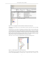
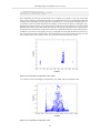
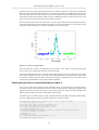
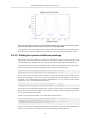
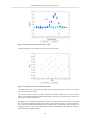
In the Beginning is the Pipeline. Photometry
images, by using a simplified version of the drizzle method
(Fruchter and Hook, 2002, PASP,
114, 144). It can
be applied to raster and scan map observations without particular
restrictions.
The only requirement is that the input frame class must
be astrometric calibrated, which means,
in the PACS case, that it must
include the cubes of sky coordinates of the pixel centers. Thus,
photAddInstantPointing and
photAssignRaDec should be executed before
PhotProject. There is not any particular treatment
of the signal in terms of noise
removal. The 1/f
noise is supposed to be removed before the execution of this task,
e.g.
by the previous steps of the pipeline in the case of
chooped-nodded observations and by the
photHighPassFilter or similar tasks in the scan map
case. The tasks projects all images
onto a map with a pixel size
defined using the "outputPixelsize" option. Note, that the option
"calibration=True" must be set in order to properly conserve fluxes of
image that are not using
native pixel sizes (3.2 in the blue and 6.4
in the red). The photProjectPointSource() is specific
version of
photProject for the chopped/nodded point source AOT style
observations.If the
allInOne=1 is set then the task create a final map
by combining both chop and nod positions (4
images altogether) and
rotate the image so that North is up and east is left. World
Coordinate
System data are produced for a later FITS file generation
of the final product.
map1 = photProject(framesnod,outputPixelsize=3.2,calTree=calTree,calibration=True)
map2 = photProjectPointSource(myframe,
allInOne=1,outputPixelsize=3.2,calTree=calTree, calibration=True)
Display(map1)
Display(map2)
product = simpleFitsWriter(map1,"filename"+str(i)".fits")
product = simpleFitsWriter(map2,"filename"+str(i)".fits")
Since there are three additional copies made of the final
dithering corrected product, the final map
contains additional images
of the source, but only the one in the centre is considered to be the
relevant result. Besides the final image, the task creates additional
products: i) error map:
distribution of errors propagated throughout
the data reduction; these errors do not reflect the
statistical error
of the final image, but also includes systematic uncertainties. As a
result,
the values usually overestimate the photometric error in the
final image. ii) coverage map: gives
the number of detector pixels
that have seen a certain logical, rebinned pixel in the final image
iii) exposure map: similar to coverage map, but this time it gives the
total observing time
spent on each logical, rebinned pixel in the
final image
You can check the result of the projection by looking at the
data using the 'Display' task. Don't
forget that in most cases you
will have more than one slices so name your files in a way that you
can retrieve them easily. (See in the example)
The difference between the two task can be seen in the two
example
different map created in the above
map1 = photProject() gives a de-rotated map (equatorial, N up, E
left) that contains all individual
frames co-added to one, showing the
characteristic four point chop nod pattern. Advantage:
more
homogeneous coverage of the sky background for determining the
background noise.
Disadvantage: S/N ratio of one individual image of
the target is a factor of two lower than the
map2 product.
map2 = photProjectPointSource() applies a simple shift-and-add
algorithm to combine all images
of the target into only one in order
to provide to optimised S/N ratio. The relevant results will be
in the
centre of the final map; the other eight copies are just an artefact
of the reconstruction
and should not be used. Disadvantage: The area
of homogeneous coverage is relatively narrow
and closely confined
around the source.
75