1
Hydrophone equipped mote
by Sidsel Jensen
Department of Computer Science
University of Copenhagen
June 2010
Abstract
Underwater sensor networks is a novel area within sensor networks. Recently there
has been a growing interest in underwater wireless sensor networks due to its advantages and benefits in a wide spectrum of applications in aquatic environments. The
main challenges of deploying such a network are the traditional ones of cost and limited battery resources of individual sensor nodes, but also consideration to the water
environment and the difficult access possibilities once deployed. As a result both hardware and software must be carefully designed. In this project we present the design and
implementation of a small-scale prototype for a hydrophone equipped sensor network
for long-term deployment in the arctic area.
i
Contents
1
Introduction
1.1 Application constraints . . . . . . . . . . . . . . . . . . . . . . . . . . . . .
1.2 Contribution . . . . . . . . . . . . . . . . . . . . . . . . . . . . . . . . . . .
1.3 Outline . . . . . . . . . . . . . . . . . . . . . . . . . . . . . . . . . . . . . .
2
2
3
4
2
Hydrophones
2.1 Terminology . . . . . . . . . . . . .
2.1.1 Propagation losses . . . . .
2.1.2 Causes of noise . . . . . . .
2.1.3 The Passive Sonar Equation
.
.
.
.
5
6
6
8
9
3
4
.
.
.
.
.
.
.
.
.
.
.
.
.
.
.
.
.
.
.
.
.
.
.
.
.
.
.
.
.
.
.
.
.
.
.
.
.
.
.
.
.
.
.
.
.
.
.
.
.
.
.
.
.
.
.
.
.
.
.
.
.
.
.
.
.
.
.
.
.
.
.
.
.
.
.
.
.
.
.
.
.
.
.
.
Design
3.1 Sensing . . . . . . . . . . . . . . . . . . .
3.1.1 Choosing a hydrophone . . . . .
3.1.2 Time-lapse camera . . . . . . . .
3.2 Computing . . . . . . . . . . . . . . . . .
3.2.1 Designing the HydrophoneSPOT
3.2.2 Designing the CameraSPOT . . .
3.3 Power estimation . . . . . . . . . . . . .
3.3.1 Energy harvesting . . . . . . . .
3.4 The hydrophone equipped system . . .
.
.
.
.
.
.
.
.
.
.
.
.
.
.
.
.
.
.
.
.
.
.
.
.
.
.
.
.
.
.
.
.
.
.
.
.
.
.
.
.
.
.
.
.
.
.
.
.
.
.
.
.
.
.
.
.
.
.
.
.
.
.
.
.
.
.
.
.
.
.
.
.
.
.
.
.
.
.
.
.
.
.
.
.
.
.
.
.
.
.
.
.
.
.
.
.
.
.
.
.
.
.
.
.
.
.
.
.
.
.
.
.
.
.
.
.
.
.
.
.
.
.
.
.
.
.
.
.
.
.
.
.
.
.
.
.
.
.
.
.
.
.
.
.
.
.
.
.
.
.
.
.
.
.
.
.
.
.
.
.
.
.
.
.
.
.
.
.
.
.
.
11
11
12
14
19
21
22
22
24
24
Implementation
4.1 Building the prototype . . . . . . . . .
4.1.1 Building the hydrophone . . .
4.1.2 Building the pre-amplification
4.1.3 Connecting the hardware . . .
4.2 Prototype limitations . . . . . . . . . .
4.3 Data post-processing . . . . . . . . . .
.
.
.
.
.
.
.
.
.
.
.
.
.
.
.
.
.
.
.
.
.
.
.
.
.
.
.
.
.
.
.
.
.
.
.
.
.
.
.
.
.
.
.
.
.
.
.
.
.
.
.
.
.
.
.
.
.
.
.
.
.
.
.
.
.
.
.
.
.
.
.
.
.
.
.
.
.
.
.
.
.
.
.
.
.
.
.
.
.
.
.
.
.
.
.
.
.
.
.
.
.
.
.
.
.
.
.
.
.
.
.
.
.
.
26
26
27
27
28
29
29
.
.
.
.
.
.
5
Test and evaluation
31
6
Conclusion
34
ii
CONTENTS
A Source code
A.1 Arduino code . . . . . .
A.2 Processing code . . . . .
A.3 HydrophoneSPOT code
A.4 HydrophoneHOST code
CONTENTS
.
.
.
.
.
.
.
.
.
.
.
.
.
.
.
.
.
.
.
.
.
.
.
.
1
.
.
.
.
.
.
.
.
.
.
.
.
.
.
.
.
.
.
.
.
.
.
.
.
.
.
.
.
.
.
.
.
.
.
.
.
.
.
.
.
.
.
.
.
.
.
.
.
.
.
.
.
.
.
.
.
.
.
.
.
.
.
.
.
.
.
.
.
.
.
.
.
.
.
.
.
.
.
.
.
.
.
.
.
.
.
.
.
37
37
38
40
47
Chapter 1
Introduction
The surface of our globe is covered by 70 percent water, yet doing underwater data
acquisition is cumbersome. The traditional approach for remote ocean monitoring is to
deploy underwater sensors that record data during the monitoring mission, and then
at a later point recover the instruments, but this approach has a number of disadvantages1 .
• Real time monitoring is not possible.
• No interaction is possible between onshore control systems and the monitoring
instruments.
• If failures or misconfigurations occur, its not possible to detect it before the retrieval of the instruments
• The amount of data is limited by the capacity of the onboard storage devices
Underwater sensor nodes and networks enable real time applications for oceanographic data collection, pollution monitoring and offshore exploration, but the water
also introduces a number of challenges for sensor network systems, such as low communication bandwidth, large propagation delays, floating node mobility and high error probability. The lifetime of the application is limited by the battery capacity and the
limited energy harvesting possibilities (solar energy and wave-generation). And the
underwater sensors themselves are prone to fouling and corrosion.
1.1
Application constraints
To make matters worse the environmental conditions in the arctic area are harsh. Sensor
networks primarily has four types of sensor activities (sensing, transmitting, receiving,
and computing), which are all put to the test in extreme weather conditions. MANA2
1
2
http://www.ece.gatech.edu/research/labs/bwn/UWASN/
http://www.itu.dk/mana/
2
1.2. CONTRIBUTION
CHAPTER 1. INTRODUCTION
is a research project with the goal of improving scientific data acquisition in polar regions. The goal of this project is to explore the possibility of adding a hydrophone equipped
sensor network mote to the current MANA research installation located in a freshwater lake
in North-East Greenland.
Hydrophones are highly versatile sensors with many possible functions, as their sensing capabilities can vary from pure sound monitoring as an aid to the study of marine
life and the environment, to seismic activity, localization as a sonar or as underwater
communication devices.
The design of the hydrophone equipped sensor network will be bound by a number
of hard requirements as well as the effect of the arctic deployment environment. The
solution should be able to operate under the following conditions and constraints:
• It will be deployed in a freshwater lake in North-East Greenland (GPS coverage
is low in the polar regions)
• The temperature range will be from +20 to -40 degrees Celcius
• The depth of the lake is about 6 meters with ice covering the lake during winter
with about 2 meters thickness
• We are looking for a passive hydrophone system
• We wish to listen after underwater and surface noise, not any kind of marine life
• The solution should be able to operate autonomously for about a year, with only
one or two maintenance checks a year
• The solution should provide real time data from the system
• We need to add a control-system to sanity-check the acquired sound data - in this
case a time-lapse camera mounted at the shores of the lake
• And it shouldn’t be too expensive
1.2
Contribution
The use of sensor networks in aquatic environments has been quite limited, partially
due to the harsh underwater environments and associated high system costs. Hydrophones, as a sensor, have only recently been integrated into underwater sensor network installations and testbeds, despite the fact that they are well-known and powerful
tools for leveraging the task of localized sound monitoring underwater.
We present the design and implementation of a small-scale prototype for a hydrophone
equipped sensor network for long-term deployment under the extreme weather conditions in the arctic.
3
1.3. OUTLINE
1.3
CHAPTER 1. INTRODUCTION
Outline
In the first part of this project we review a small but relevant part of the terminology
regarding hydrophones (Chapter 2) and describe and analyze the design space and corresponding design choices (Chapter 3). In the second part we discuss the implemented
prototype (Chapter 4) and conducted tests (Chapter 5) and in the third and final part
we will evaluate and conclude on the findings (Chapter 6).
4
Chapter 2
Hydrophones
A transducer is an electronic device that converts energy from one form to another,
whereas a SONAR (SOund NAvigation and Ranging) is a technique which uses sound
under water to navigate or detect other vessels. The sonar works after the same echoprinciples as a RADAR (RAdio Detection And Ranging). Sonars are classified into two
main categories depending on their mode of functioning:
Active sonars - transmitting a signal and receiving echoes from a target. The measured time delay is used to estimate the distance between the sonar and its target
and receiving the signal on a suitable antenna completes the measurement with
a determination of the angle of arrival of the signal. Active sonars are also called
projectors.
Passive sonars - are designed to intercept noises (and possible active sonar signals)
radiated by a target vessel. Their main interest lies in their total stealth. Passive
sonars are also called hydrophones.
The first underwater echo detection systems were developed by British, American
and French scientists for the purpose of underwater navigation by submarines in World
war I and in particular after the Titanic sank in 1912. Their two primary functions was
to locate submarines and icebergs, but these earliest systems, only worked at relatively
high frequencies, and achieved detection ranges of only several thousand yards under favorable conditions. Between the two world wars the sonar technology improved
considerably. It benefitted from the emergence of first-generation electronics and from
progress in the newborn radio industry. In the aftermath of World War II, the Cold War
between the Western and the Eastern blocks, ensured continued focus on the efforts in
the scientific and technological research on underwater acoustics[2].
In parallel with military developments oceanography and industry were able to profit
from the development of underwater acoustics. For instance the invention of the sonic
depth finder (SDF) in the early 1920s, facilitated a detailed depth and ocean-bottom
5
2.1. TERMINOLOGY
CHAPTER 2. HYDROPHONES
surveys with a speed and accuracy never before available using the traditional leadline techniques to measure water depth. Several systems became wide spread and are
today used as both scientific instrumentation and indispensable navigation tools.
2.1
Terminology
Acoustic waves originate from the propagation of a mechanical perturbation. Local
compressions and dilations are passed from one point to the surrounding points because of the mediums (the water) elastic properties. The propagation rate of the perturbation of the medium is called the velocity. But the propagation velocity of an acoustic
wave is also imposed by the characteristics of the propagation medium - it depends on
the density p and the elasticity modulus E[1].
c=
q
E
p
In sea water, the velocity of the acoustic wave is close to c = 1.500 m/s, with small
variations due to pressure, salinity and temperature. The density of sea water is approximately p = 1.030 kg m−3 . Fresh water has the density of p = 1.000 m−3 , so sea
water is about 3% more dense than fresh water. This compared to air where the respective values of sound velocity and density are approximately 340 m/s and 1.3 kg m−3 .
Water has the anomalous property of becoming less dense, not more, when it is cooled
down to its solid form, ice. It expands to occupy a 9% greater volume in this solid state,
which accounts for the fact of ice floating on liquid water.
Acoustic signals are characterized by the number of vibrations per second - the frequency f expressed in Hertz. The frequencies used in underwater acoustics range
roughly from 10 Hz to 1 MHz, depending on the application.
For a sound velocity of 1.500 m/s, the underwater acoustic wavelengths will be 150
m at 10 Hz, 1.5 m at 1kHz and 0.0015 m at 1 MHz.
2.1.1
Propagation losses
The propagation of a sound wave is associated with an acoustic energy, expressed as
either the acoustic intensity I or the acoustic power P . Intensity and power can vary enormously. A high-power sonar transmitter may deliver acoustic power of several tens of
kilowatt, whereas a nuclear submarine in silent mode might radiate only a few milliwatts. When acoustic waves propagate, the most visible process is their loss of intensity
because of geometric spreading (a divergence effect) and absorption of acoustic energy
by the propagation medium itself. This propagation loss or transmission loss is a key
parameter for acoustic systems. Sea water is a dissipative propagation medium - it
absorbs part of the energy of the transmitted wave. We also call the gradual loss in
6
2.1. TERMINOLOGY
CHAPTER 2. HYDROPHONES
Figure 2.1: Frequency ranges of the main underwater acoustic systems [1]
intensity of any kind of flux through a medium for attenuation.
Because the propagation medium is limited by the sea surface and the seabed, the
signals transmitted undergo reflections at the interfaces. Any given signal can therefore
propagate from source to receiver along several distinct paths (multiple paths). The main
signal arrives along with a series of echos, of amplitudes decreasing with the number
of reflections undergone. It is called backscattering, when the reflection of an acoustic
wave collide with an obstacle in the water or at the limits of the medium and reflects
the acoustic wave and send an echo of the signal back to the direction they came from.
It is a diffuse reflection, as opposed to a specular reflection like a in a mirror. The
time structure of the signal is somewhat affected and the performance of a system can
be highly degraded by these parasite signals. Depending on the application the echoes
can be either desirable or undesirable - if they are completely jamming the useful signal.
In general there are four factors that are peculiar to the arctic environment which complicate the modeling of acoustic propagation:
1. the ice keels present a rapidly varying surface
2. the reflection, transmission and scattering properties at the water-ice interface are
not well known
3. the measurement of under-ice contours is difficult and
4. the diffraction of sound around ice-obstacles may be important
Due to scattering at the rough boundaries of the ice, only low frequencies (typically
less than 40 Hz) can propagate to long distances in the Arctic channel.
7
2.1. TERMINOLOGY
2.1.2
CHAPTER 2. HYDROPHONES
Causes of noise
Noise is an important component of underwater acoustics. The cause of noise can be
grouped into four categories:
• Ambient noise - typically originates from factors outside the system and stems
from natural or man-made causes.
• Self-noise - typically from the systems own electronics
• Reverberation - typically caused by parasite echoes, but only affects active sonar
systems
• Acoustic interference - typically generated by other acoustic systems nearby.
The two first categories are the ones most likely to cause interference in our system.
By definition, ambient noise is the noise received by the sonar in the absence of any
signal and self-noise from the system. Ambient noise has several very distinct physical
origins, each corresponding to particular frequency ranges:
• Seismic and volcanic activity (very low level frequencies)
• Shipping and industrial activity (from 10Hz - 1kHz)
• Surface agitation depends on sea state and wind speed. (from a few hertz to a few
tens of kHz)
We don’t anticipate any noteworthy seismic and volcanic activity close to our system and shipping will not pose a problem, as the hydrophone is to be deployed in a
freshwater lake. Surface agitation on the other hand - will prove very interesting to
measure.
Air bubbles are created by sea surface movements for instance by heavy rain and cause
ambient noise. They form an inhomogeneous layer close to the surface, whose dualphase mixing modifies locally and strongly the acoustic characteristics of the propagation medium (velocity and attenuation). This process decreases in importance as depth
increases, because the hydrostatic pressure increases. Below 10 - 20 meters the effect of
bubbles can be neglected.
In the mid-frequency band (200 Hz - 50 kHz), the dominant noise source is wind acting
on the sea surface. It has been shown, that there is a strong correlation between ambient noise and wind force or sea state. Ambient noise increases about 5dB as the wind
strength doubles. Peak wind noise occurs around 500 Hz, and then decreases about
-6dB per octave.
8
2.1. TERMINOLOGY
CHAPTER 2. HYDROPHONES
Frozen lakes are known to give off most noise during major fluctuations in temperature: the ice expands or contracts, and the resulting tension in the ice causes cracks
to appear. Due to the changes in temperature, the hours of morning and evening are
usually the best times to hear these sounds. Thin ice is especially interesting for acoustic phenomena; it is more elastic and sounds are propagated better across the surface.
Snowfall, on the other hand, has a muffling effect and the sound can only travel to a
limited extent. The ice sheet acts as a huge membrane across which the cracking and
popping sounds spread.
2.1.3
The Passive Sonar Equation
The sonar equations are founded on the basic equality between the desired (signal) and
undesired (background) portions of the received signal. For a sonar to successfully
detect an acoustic signal we require that it is above a detectable threshold (DT) :
SignalLevel > BackgroundLevel
Signal to noise ratio is an important concept because it represents the degree to
which an amplifier can be successfully employed to improve the situation. If the signal
to noise ratio (S/N or SNR) is too low, the noise is nearly equal to the signal. In this
case, amplification will also increase the noise and provide no substantial improvement.
For high signal to noise ratios, amplification will improve the magnitude of the signal
relative to the noise. We can express this correlation with the passive sonar equation:
SN R = SL − T L − N L + DI
where SL is the source level, TL is the transmission loss, NL is the noise level, and
DI is the directivity index. The directivity index DI for our network is zero because we
assume omnidirectional hydrophones. All the quantities in the equation are in dB re
µPa, where the reference value of 1 µPa amounts to 0.67 × 10⁻²² W atts/cm2 .
SL = 10log IIS0
IS = Signal Intensity
I0 = Reference Intensity - 1 µPa
The origin of these two terms is the intensity of the signal that is transmitted to the
water from the target. This is called the Source Level (SL).
T L = 10log IIRS (For a plane wave)
IR = Received signal intensity
As the signal travels through the water, some of the signal is lost through various
propagation losses. The totality of this loss is quantified as the Transmission Loss (TL).
As a general rule, Transmission Loss is dependent on the distance between the source
and the receiver.
9
2.1. TERMINOLOGY
CHAPTER 2. HYDROPHONES
N L = 10log IIn0
In = Noise intensity
The Noise Level (NL) is the sum of the total effect of background and self-noise
hindering our ability to detect the target signal. An average value for the ambient noise
level NL of 70 dB is a representative of the shallow water case[4].
Figure 2.2: The Passive Sonar Equation
10
Chapter 3
Design
In the following we will analyze how to design the hydrophone equipped sensor network. It’s important to realize that the hydrophone equipped mote will at some point
be part of the existing research installation at Zackenberg, and some consideration to
the current setup and infrastructure should be taken. For instance, there is already a
buoy in the lake with an Arc rock based IPSerial mote inside[5], which might have
space for the hydrophone equipped mote too. If not, another buoy should be bought
for the deployment of the hydrophone into the lake. Also there is a GW installation on
the shore of the lake, with a working wireless connection to the research station some 4
km away. A side from that, the proposed solution will be autonomous from the existing
one, to allow maximum independence in case of system failures.
3.1
Sensing
We wish to design and build a sensor network system, centered around the input from
two sensors: a hydrophone deployed in the lake and a time-lapse camera mounted
on the shore of the lake. The sensor node controlling the hydrophone will wake up
at timed intervals and make sound recordings which will be sent to the GW. In order
to be able to control and match the sound recordings against some ground truth, we
wish to take at least one time-lapse picture a day on which the current weather condition around the lake can be seen. The time-lapse camera provides our eyes in the
field during the remote monitoring mission. It is our hope, that we later during the
post-processing of the sound recordings can match the recordings to a certain weather
situation and a specific noise in the recording.
It might also be a good idea to mount a small weather sensor, so we can pickup on
for instance wind speed or very large differences in temperature. So if the wind speed
stays above a certain threshold for a longer period which could be a favorable condition for our sound monitoring, we wish to wake up our sensor nodes to perform extra
11
3.1. SENSING
CHAPTER 3. DESIGN
measurements. We cannot afford energy wise to do this very often, but it will most
likely provide us with recordings of extreme situations, which can help set the normal
recordings into the right context and give us a larger data set which will provide more
detail and precise information. Preferably the data set from the first 6 months should
be used to debug and fine tune the system for the next deployment period.
3.1.1
Choosing a hydrophone
For the sake of simplicity we have selected 4 hydrophones for consideration - two in
the cheap range: the Aquarian H2A hydrophone1 and the DolphinEAR2 and two in
the expensive range: a RESON3 TC4032 and a Brüel and Kjær4 8103 Miniature Hydrophone. They are all omni-directional and passive listening devices. All four are
from well known companies and very reliable.
Aquarian
DolphinEAR
RESON
Brüel and Kjær
Description
H2A
DE100 Series
TC4032
8103 Miniature
Frequency
10 Hz - 100KHz
7 Hz - 22 kHz
5Hz to120kHz
0.1Hz to 180 kHz
Power
0.3 mA
Approx 7 mA at 9V 19mA at 12VDC
6mA without load
Sensitivity
-180dB re 1V/µPa
-170dB re 1V/µPa
-211 dB re 1V/µPa
Connector
3.5 minijack
3.5 minijack
LEMO
10-32UNF microdot plug
Pre-amplifier internal imp. buffer amp external PA amplifier low-noise 10dB
external amp
Cable
not included
8m
6m
10 m
Price
159$
319 $
DKK 17.887,00
-
Table 3.1: Comparison of 4 different hydrophones
We will be doing measurements about 3 meters down in the lake, free from the ice
cover, which is roughly 2 meters thick during the winter. The lake is about 6 meters
deep, so this would put the hydrophone right in the middle between the water surface
and the lake bottom. The two expensive hydrophones are built to withstand deep underwater pressure of 500 m depth or more. Since we are doing our measurements in
what may be characterized as shallow water, the extra endurance of the expensive hydrophones might not be necesarry. However the hydrophone might still get trapped in
the ice during spring when the ice melts and refreezes and extra care needs to be taken
to protect the wire connecting the hydrophone to the mote, as the ice can be very sharp.
The wire should be packed in an isolating pipe (which shouldn’t make too much noise
when crushed) to relief some of the pressure from the ice, which will form around it
during the winter. A good design choice could be to go for one of the cheaper type of
1
http://www.afabsound.com/home.php
http://www.dolphinear.com/de-specs.htm
3
http://www.reson.com/sw3154.asp
4
http://www.bksv.dk/Products/TransducersConditioning/AcousticTransducers/Hydrophones/
2
12
3.1. SENSING
CHAPTER 3. DESIGN
hydrophones or build one ourselves since there is a high risk of loosing it during winter.
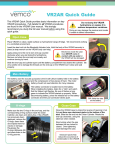
Figure 3.1: The DolphinEAR De100 hydrophone
Looking at the coating of the four hydrophones all three but one looks very sturdy.
The DolphinEAR is not packed in the same hard cover as the rest of the hydrophones
- its piezoelectric membrane is much more exposed, which means it might be unfit for
an arctic deployment. The missing coating will also make it much more exposed to
corrosion during the year long deployment, compared to the other three.
When listening for noise it’s a good idea to choose the broadest possible frequency
bandwidth, but that costs power. The DolphinEAR is the hydrophone with the smallest frequency span, whereas the Brüel and Kjær hydrophone has the broadest frequency
span. They are all however, within the frequency span, which is relevant for noise observations. They all claim to have low-self noise, which is important when listening for
ambient noise. We want to be able to hear the signal, it shouldn’t drown in electro-static
noise from the system itself. You normally apply a high pass filter over the recording
to remove the noise, but this might not be possible as we then might also remove the
valid noise signal we are listening for.
The power requirement is highly relevant for the lifetime of the application. Increasing the intensity and the pre-amplification of the hydrophone signal requires higher
power. The higher power drain combined with the arctic environment with below 0
temperatures for half a year at a time will most likely deplete the battery faster than
we anticipated. A device called a battery guard5 might be worth considering into the
setup. These are voltage monitoring devices that vary in complexity and capability and
they prevent the excessive discharge of the battery (which would damage the battery)
and protects electronic appliances against over- voltage. They can turn off any device
operated through it when the battery voltage drops below a critical point. On the other
5
http://www.elfrasolen.dk/Produkter/Batterivagt/index.htm
13
3.1. SENSING
CHAPTER 3. DESIGN
hand - the battery might be the cheapest part of the whole design, and we want to keep
on sampling for as long as absolutely possible, even if that means depleting the battery
completely. It might be a better solution to choose a smaller dynamic frequency range
and a small sample rate to reduce the power drain.
Figure 3.2: The Aquarian UP1 pre-amplifier inside
The signal we receive from the hydrophone will most likely need some sort of preamplification, otherwise it will be too weak. Usually a professional external amplifier is
used to enhance the signal further, but including that in the on site setup is not recommendable. It would require even more space for hardware and even more power. The
RESON hydrophone comes with a built-in 10dB pre-amplifier, and with the DolphinEAR a small external amplifier is included, but mostly the hydrophone suppliers lets
you buy the pre-amplifiers as an extra accessory. Instead of buying one, we could also
build one ourself and integrate the preamplifier into an add-on sensor board placed on
the sensor node. We will need an add-on board anyway, since we need to connect the
the hydrophone to the sensor node.
Our recommendation would be to go for a cheaper hydrophone fx. the Aquarian
H2a6 . It’s sturdy, cheap and has a low power consumption, which makes it ideal for our
usage. The price for the Aquarian H2a hydrophone does not include pre-amplification
or cables, but it still has a price well below the RESON hydrophone. The low price,
also means that an extra spare can be bought, so should the hydrophone be damaged
during winter, it can be changed at the first possible maintenance check without loosing
the possibility of doing measurements the rest of the year.
3.1.2
Time-lapse camera
Our second sensor for the system is a time-lapse camera, which should be mounted
on the shores of the lake. Harbortronics7 sells such a complete time-lapse package for
6
7
Its also the primary choice for many hobby recording artists, which illustrates its ease of use
https://www.harbortronics.com/Products/TimeLapsePackage/
14
3.1. SENSING
CHAPTER 3. DESIGN
Figure 3.3: The Aquarian H2A hydrophone with external pre-amp
remote monitoring. The solution includes:
• Fiberglass Housing, glass window
• High capacity internal Lithium-Ion Polymer battery pack.
• 5 Watt Solar Panel
• Harbortronics Solar Charger
• Harbortronics Battery Converter
• Harbortronics DigiSnap 2100
• Canon Rebel XS (1000D) camera
• A pair of 8 GB memory cards
• All required tools, cables, manuals and accessories
The enclosed camera is a Canon Rebel XS (1000D) which shoots with 10.1 Megapixel,
with a maximum resolution of 3888x2592 pixels. There’s the choice of two lower resolutions, and all three sizes can be recorded with either Fine or Normal JPEG compression.
Its also possible to record RAW files either with or without a Large Fine JPEG. Best
quality Large Fine JPEGS typically measure between 3.5 and 4 MB each, while RAW
files measure around 10MB each. Shooting in RAW format and saving them on the 8
GB SD card gives us room for about 800 pictures, but if we choose Large Fine JPEGs we
have room for more than twice as many pictures, roughly 2000. With the RAW format
we can do two pictures a day, with the Large Fine JPEGs we can take five pictures a day
for a whole year without filling up the card entirely. But SD cards comes cheap these
days, so we would recommend buying a pair of 32 GB cards, leaving plenty of room
15
3.1. SENSING
CHAPTER 3. DESIGN
Figure 3.4: The Harbortronics Time-Lapse package
for pictures. Energy tests in the lab should be performed to see how much power is
consumed by powering on the camera, taking a picture and shutting it down again, to
measure what is the safe limit for how many pictures can be taken, if the solution is to
operate at least 6 months without human interference.
The perhaps most important device apart from the camera itself, is the Digisnap 2100,
which controls the camera trigger. The DigiSnap can be configured for either A Simple
Time-Lapse (STL) sequence, which consists of an initial delay, followed by a number of
pictures taken with a particular interval between each picture or an Advanced TimeLapse (ATL) sequence, where a set of Time-Lapse sequences can be programmed to
start at particular times of the day, but the DigiSnap controller does not have a ’realtime’ internal clock, so once powered up it will presume that it’s midnight. In terms of
connectivity, a flap on the left side of the camera body opens to reveal the TV output, a
socket for the optional RS-60E3 remote switch and a USB port. The Digisnap controller
connects to the shutter release jack (the RS-60E3 pinout). The interface is very simple,
generally just a switch contact. The Digisnap controller is configured by connecting a
null-modem cable between the controller and a PC/Mac and using a simple terminal
program.
Energywise the package comes equipped with a single high capacity Lithium-Ion Polymer (LiPoly) rechargeable battery pack, having a nominal voltage of 11.1V, and 9AH capacity. The fully charged LiPoly battery pack has enough capacity for about 2 months of
operation between charges, depending on the details of the application. The most common battery chemistry for long term, remote applications is lead-acid. Unfortunately,
16
3.1. SENSING
CHAPTER 3. DESIGN
lead-acid batteries have a number of drawbacks - they are large and heavy and they
can vent gases during charge and discharge, making them inadvisable to install within
a sealed housing. Most other secondary (rechargeable) battery chemistries have high
self-discharge, meaning that they won’t work well in a long term application. LiPoly
batteries however, have low self-discharge, are very light-weight, and quite compact.
The Digisnap controller operates on an internal 5V supply, but is typically also powered by the LiPoly battery-pack though the battery converter. When the DigiSnap is
off, there is a load of 8-10 uA on the battery. For the lowest power consumption, the
camera should be configured to not turn the LCD back display automatically on, as it
is a sure battery drain, but also to set the following options:
• Auto power off : 1 minute
• Manual focus: Shake Reduction Off
The solution also includes a 5W solar panel, which can be exchanged for a larger
panel if necessary. At Zackenberg which is located at (74◦ 30’N / 21◦ 00’W) in NorthEast Greenland 25 km north-west of Daneborg, there is a partial midnight sun in the
period from May 2nd - August 12th. Its four months of summer and 8 months of winter
darkness. While the 5W solar panel will be more than enough to recharge the battery
during the summer, it could be a good design choice to have a larger 20W solar panel8
for the transition into winter, so it’s possible to recharge the batteries even with fewer
hours of light. The solar charger, that comes included in the time-lapse package can
be reused. Harbortronics recommends that the solar panel rests on top of the housing,
where it can also serve as a rain shield to minimize drops on the front window of the
housing. With a larger solar panel, that might not be possible, if the solar panel should
be placed in the optimal 45 degree angle.
Apart from shielding the wires from wildlife, the user guide gives no other indications
as how to shield the box from the arctic environment. A snow storm might possibly
cover the window, with snow and ice, leaving the camera ’blind’. It will most likely be
worthless to isolate the box itself, as the cold would still penetrate the glass window,
but isolating the battery could prove a good investment for the battery-lifetime.
The Harbortronics solution seems very stable. The university of Alaska has tested the
system at low temperatures in their facilities and they found that the system worked
all the way down to the lowest tested temperature, -60C. However, at –40C and below,
some pictures were missing from the sequence. Some of the pictures were dark, others
half light / half dark, suggesting that the mechanical items in the camera, the shutter
and the mirror assemblies may have been sticking at times, or otherwise slowed. The
timing never varied, suggesting that all of the electronics worked at all temperatures
even though the normal operating temperature of most digital SLR cameras is specified
for 0C to +40C.
8
http://dk.farnell.com/solar-panels
17
3.1. SENSING
CHAPTER 3. DESIGN
The Harbortronics system is an ideal solution for the traditional way of doing remote
autonomous monitoring, but it does not provide any hooks for real time data retrieval.
Direct simple connection to s sensor network system is not possible, which leaves us
with several options. Either the Digisnap 2100 can be replaced with a Digisnap 2800
which includes an external input/output wire where we can connect the sensor node,
allowing the sensor node to control the Digisnap, which in turn controls the camera,
but a simpler solution might be to remove the Digisnap controller altogether and let
the sensor node and its internal clock control the time-lapse sequence of the camera
through the shutter release jack.
To retrieve the data we must also connect a USB cable to the camera. A large number
of SLR cameras support the Picture Transfer Protocol (PTP) for bulk transfer - which
is a widely supported protocol developed by the International Imaging Industry Association to allow the transfer of images from digital cameras to computers and other
peripheral devices without the need of additional device drivers. The protocol has been
standardized as ISO 15740. But no sensor nodes, that we are aware of, support the protocol at this point in time. PTP is supported on Linux and other free software/open
source operating systems such as FreeBSD by a number of libraries, such as libgphoto
and libptp as well as the application Gphoto29 .
In order to get PTP or PTP/IP working, we’ll need a very small scale computer with an
operating system and a USB port to transfer the images from the camera to the research
station through the wireless connection. That could be either a Fit-PC210 or Linux on a
Gumstix11 (fx. the Overo Air model), both are probably small and low-power enough
to fit inside the fiberglas housing.
But at this point the whole time-lapse solution is getting rather complicated with
many separate parts and many possibilities for independent failures. It might be worth
looking for a simpler solution with fewer parts. One such simpler solution could be the
Campbell Scientific CC640 digital camera12 for use in harsh environments. The CC640
operates at temperatures as low as -40◦ C, and image acquisition can be triggered by
applying a 5 to 12-volt signal. Images are stored on a CompactFlash card or in a datalogger’s memory. The images are stored in a JPEG format, but unfortunately only in
640 x 480 (307,200 pixels) resolution, which is nowhere near the good resolution of the
canon SLR camera. The camera is powered by 9 to 15 V with a power drain of 250 mA
maximum (operating) and 250 uA typical (quiescent). The camera uses the Pakbus protocol13 to transfer images. The camera works as a PakBus Leaf node and is not capable
9
http://www.gphoto.org/
http://www.fit-pc.com
11
http://www.gumstix.com/
12
http://www.campbellsci.com/cc640-digital-camera-specifications
13
http://www.campbellsci.com/documents/manuals/pakbusnetguide.pdf
10
18
3.2. COMPUTING
CHAPTER 3. DESIGN
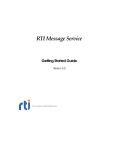
Figure 3.5: The Campbell Scientific CC640 digital camera
of performing any routing. The camera could be connected to a sensor node through
the cameras RS-232 output, but in order to retrieve the images, the sensor node would
have to understand the Pakbus communication protocol to fetch the images.
Which solution to go for depends on whether the captured images should be retrieved
in real time or not. If we just want to control when the pictures are taken, but not retrieve the pictures until the first maintenance check, the Harbortronics solution would
be perfect. However if the image data needs to be retrieved periodically, we would
recommend to look for a different solution.
3.2
Computing
The existing sensor network at Zackenberg uses the Arc Rock IPserial nodes for computing. The benefit of the Arc Rock nodes14 is that they offer a whole range of ICMP
control and management messages as well as support for full UDP and TCP transportlayer protocols as well as over-the-air (OTA) programming. For the easiest integration
it would be best to choose a similar node for the new setup.
However the chip driving the IPserial node is not particularly strong, and some
pre-processing on the node might be necessary with the hydrophone as it’s sampling at
a high data-rate, so the the SunSPOT sensor node platform15 , from Sun Labs, Sun Microsystems (now Oracle) might be worth considering. If offers a 180 MHz ARM-based
CPU with 512 KB RAM and 4MB flash. It also offers over-the-air programming and
by the end of the summer 2010, it will have a working IP6 stack on top of the 6LoWPAN protocol16 . It also features different mesh networking protocols. The SunSPOT
14
http://www.archrock.com/technology/faq.php
http://www.sunspotworld.com/
16
http://blogs.sun.com/roger/entry/summer research assistants 2010
15
19
3.2. COMPUTING
CHAPTER 3. DESIGN
Figure 3.6: The SunSPOT from Sun Microsystems
processor board features:
• 180 MHz 32 bit ARM920T core - 512K RAM/4M Flash
• 2.4 GHz IEEE 802.15.4 (a CC2420) radio with integrated antenna
• USB interface
• 3.7V rechargeable 720 mAh lithium-ion battery
• 32 uA deep sleep mode
and the general purpose sensor board (the eDemo board) features:
• 2G/6G 3-axis accelerometer
• Temperature sensor and light sensor
• 8 tri-color LEDs
• 2 momentary switches
• 6 analog inputs
• 5 general purpose I/O pins and 4 high current output pins
Also the SunSPOT offers a range of easy to use add-on boards, allowing us to transform the SunSPOT for instance into an efficient datalogger, by using the eFlash add-on
board.
20
3.2. COMPUTING
CHAPTER 3. DESIGN
Figure 3.7: The SunSPOT eFlash and ePrototype add-on boards
3.2.1
Designing the HydrophoneSPOT
The output from the hydrophone should be connected to one of the sensor nodes Analog to Digital Conversion (ADC) input pins. The SunSPOT comes equipped with the
eDemo sensor board which includes the analog device ADT7411 for ADC conversion.
The internal oscillator circuit used by the ADC has the capability to output two different clock frequencies. This means that the ADC is capable of running at two different
speeds when doing a conversion on a measurement channel. Setting the ADC into single channel mode in SPOT software will change the default sampling rate from 1.4Hz
and make the ADC sample at the specified channel every 44.5 microseconds (= 22.5
kHz), although the SPOT will probably not be able to read it faster than every 142 microseconds (= 7.042 kHz) plus whatever loop overhead is needed. So the practical max
sample rate using the eDemo board will probably be under 6.9 kHz and, but it would
be better to sample faster than that. One option could be to unplug the eDemo board,
and stack both the eFlash board and the ePrototype board on top of the SunSPOT. The
eFlash board will be used for storage of the acquired data and the ePrototype board
for connecting the analog device TI AD7710 which can sample the input signal at a frequency of 39 kHz or greater. This unit was successfully used in the breakout boards of
the sensor network doing real time volcano monitoring in Ecuador[9]. Also the ePrototype board can be used for building our own pre-amplifier, with complete control over
the gain of the amplification and a tight coupling of the hardware parts.
The benefit of storing the acquired data on the sensor node, allows us to finish sampling before transmitting the data wireless to the GW. The result being, that we can
have a high sampling rate without spending unnecessary clock cycles offloading the
data while still sampling. When sampling with a high data rate, it will take some time
to transfer the data. We propose a classic duty cycle, where the sensor node wake up,
does its sampling, forward the data to the GW, do a bit of administrative work like
sending information on storage used, battery level left etc, before going back to sleep.
The exact length of the sample period will depend on how much battery capacity we
can equip the node with while still keeping it inside a buoy.
21
3.3. POWER ESTIMATION
3.2.2
CHAPTER 3. DESIGN
Designing the CameraSPOT
As for building a time-lapse sensor node based controller for the camera ourselves,
several complete guides can be found17 . It will not require any noteworthy computing
efforts, but rather a pretty accurate time keeping which shouldn’t drift too much during
the year long deployment. Since the arctic circle is on the outskirts of GPS coverage, it
would be a better solution to sync its time against the GW with a fixed interval for
instance once a month, like its done in the current setup.
3.3
Power estimation
The lifespan of our application depends on how effective our strategy for using the battery will be. One of our primary requirements, is for the system to work autonomously
without human interference for at least 6 months preferably longer. As a minimum
we need to power the hydrophone, the camera and the two controlling sensor nodes
including the pre-amplifier and the eFlash boards for safe storage of data. While the
Harbortronics camera solution comes equipped with its own battery (and solar panel)
scaled for long-term deployment, the hydrophone needs powering either by itself or
through the sensor node which calls for an efficient duty cycle. The firmware of the
SunSPOT enables three different modes of operation:
Run
Idle
Deep-sleep
Basic operation with all processors and radio running. Power draw
for the eSPOT board is between 70 mA - 120 mA. The eDemo
board can consume up to 400 mA if enabled.
ARM9 clocks and the radio are shut off. Idle power consumption
is about 24 mA.
All regulators are shut down except for the standby LDO, the powercontrol Atmega and pSRAM. Deep-sleep power consumption is 32 µA.
Table 3.2: Overview of the SunsPOTs three modes of operation
Deep-sleep cannot be entered if if the radio is on, if external power is supplied or if
USB power is on. Deep-sleep and idle modes can be entered through the programming.
Waking the processor up from deep-sleep can be done with either an alarm, an external
interrupt or by pressing the attention button.
Let’s do a rough power estimate. The runtime power draw from the hydrophone
equipped sensor node will worst case be around (120 mA + 400 mA) 520 mA (but much
can be done to reduce this number). If the goal is a duty cycle of 90/10 (90 % sleep, 10
% awake) spread across a year.
17
http://www.glacialwanderer.com/hobbyrobotics/?p=13
22
3.3. POWER ESTIMATION
CHAPTER 3. DESIGN
10 % of 365 days = 36.5 days
36.5 days × 24 hours = 876 hours / 365 days = 2.4 hours per day
2.4 hours × 520 mA = 1248 mAH
The capacity of the built-in Lithium-ion battery is 720 milliampere-hours, so we
would deplete the battery by using the SunSPOT for 1.38 hours. Now let’s try to do the
calculation the other way around. Lets assume we can have the SunSPOT turned on
for a total of 1 hour over a period of half a year, after which the battery can be changed
during maintenance:
60 minutes × 60 seconds / 180 days = 20 seconds per day
If we only sample once every five days - we could do a 1 minute sample. So our
sample period will be 60 seconds.
1 hour × 520 mA = 520 mAH for the whole period
That leaves 200 mAH on the battery for deep-sleep mode.
180 days × 24 hours = 4320 hours
4320 × 32 µA = 138 mAH
which is within the 200 mAH limit. That leaves us with the task of programming
either a 99.998/0.002 duty cycle, finding a bigger battery or trying to harvest some
renewable energy! But unfortunately it doesn’t end there - we must also consider the
transmission time of the samples - if we sample at 7kHz for 60 seconds and each datapoint in the sample is one byte, we get:
7000 × 60 × 1 = 420 kBytes per minute
According to the CC2420 radio datasheet, the radio has a transmit speed of 250
kbps:
420 kBytes per minute × 8 bit / 250 kbit per second = 13,44 seconds
which means we have to reduce the sample period from 60 seconds to about 45 seconds, if we are to preserve energy for both sampling and transmitting the data!
But preferably we would like to sample with 44kHz with the Aquarian H2A hydrophone,
which will give us even more data to transfer:
44000 × 60 × 1 = 2.640 kBytes per minute
2.640 kBytes per minute × 8 bit / 250 kbit per second = 84,48 seconds
so for each one minute sample, it will take us 1 minute and 24 seconds to transfer
the data. That would require that we reduced the sampling period by more than half.
If we still want a 1 minute sample it would have to be once every fourteen days or so.
We suggest that we possibly try to find a bigger 3.7V Li-ion battery for the SunSPOTs.
23
3.4. THE HYDROPHONE EQUIPPED SYSTEM
3.3.1
CHAPTER 3. DESIGN
Energy harvesting
In order to prolong the lifetime of the application, we need to consider using the possibility for energy harvesting. Both solar panels and wind turbines have been installed
with success on bases in Antarctica proving their sturdiness in a harsh off-grid environment. The most obvious choices would be:
• solar energy
• wave power generation or
• wind power
Unfortunately wave power generation is not currently a widely employed commercial technology, and the lake is covered by ice all winter making it impossible to
effectively use this strategy for most of the year. Also setting up a wave generator in
the lake in close proximity to our buoy could generate a lot of noise, disturbing our
samples. Setting up a wind turbine near the lake is also a possibility, but the force of
the arctic storms might take it out. A solar panel will work great during the summer
months, but produce little or no power during the dark winter, even though the snow
on ground will work as a reflector for the daylight. The solar panel is probably the best
value for money solution and in fact there already is a solar panel in the current installation powering the GW during summer, but a hybrid approach combining a wind
turbine with a solar panel would probably give a better all-year yield18 . However the
solution needs to be within close proximity to our sensor node inside the buoy, which
renders using a wind turbine practically impossible, but a small flexible solar panel
might be mounted on the sides of the buoy.
3.4
The hydrophone equipped system
The proposed sensor network system consists of the following parts:
• An Aquarian H2A hydrophone + external pre-amplifier + cables ( 300 $)
• Harbortronics time-lapse camera solution (2.550 $)
• 2 sensor nodes either SunSPOTs (750 $) or Arch Rock based
• A flexible solar panel for the buoy if possible
• A hard pipe or similar for housing the hydrophone wire
• 1 eFlash and 1 ePrototype add-on boards for the SunSPOT
• 4 SD-cards - two for the camera (32 GB) and two for the SunSPOTs (2 GB)
18
http://www.wirefreedirect.com/stand alone power system design.asp
24
3.4. THE HYDROPHONE EQUIPPED SYSTEM
CHAPTER 3. DESIGN
• Hardware for building our own pre-amplifier
We estimate that the solution can be built for less than 5000 $ for the hardware parts.
The sensor network consists of two sensor nodes - one controlling the Aquarian H2A
hydrophone and one controlling the shutter control for the time-lapse camera. The hydrophone node should be placed inside a buoy in the middle of the lake with a pipe
protecting the hydrophone wire from the ice. The camera node should be placed on the
shores of the lake looking out over the lake. A solar panel is mounted on the roof of
the camera housing prolonging the lifetime of the battery for the camera. If possible a
flexible solar panel should be installed all around the top of the buoy. The hydrophone
node is equipped with two stackable add-on cards, an eFlash card for safe storage of
the acquired data on a SD-card and an ePrototype board for building our own preamplifier. The external pre-amplifier from Aquarian mentioned above is for testing
the hydrophone before attaching it to the sensor node. Battery-packs are connected to
the two sensor nodes and the camera itself. The solution is estimated to be deployed
for a whole year, with at least one maintenance window scheduled after half a year of
operation, upon which the SD-cards should be swapped and batteries exchanged for
new fully charged ones. The sensor node controlling the camera wake up once a day,
to make the camera take a picture. Radio contact is established with the GW once a
month to sync time. The sensor node controlling the hydrophone wakes up every 14
days to make a 45 second sample. The data is sent by radio to the GW. Data can be
transferred by wifi from the GW to the research camp 4 km away. Depending on the
quality and speed of the satellite link from the research camp, data can be forwarded
further if possible.
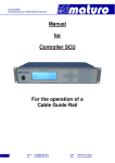
Figure 3.8: Overview of the hydrophone based sensor network setup
25
Chapter 4
Implementation
In the following we will take a look at the actual implementation of the prototype for
the HydrophoneSPOT and a corresponding GW application the HydrophoneHOST.
We built the prototype in order to obtain some knowledge on the performance of the
system, without having access to all the right hardware parts. The result being, that
some of the knowledge gained in this process can be directly transferred to the final
system, while other parts will have to be redone once the final system is complete.
4.1
Building the prototype
We built the prototype using the Arduino Duemilanove board1 and a breadboard. The
Arduino2 is an open-source electronics prototyping platform based on flexible, easyto-use hardware and software and using it allowed us to quickly build the hardware
while still being able to test it. The finished hardware on the breadboard was then
transferred from the Arduino to the SunSPOT, where the actual code for the application
was written.
Figure 4.1: The Arduino duemilanove prototype board
1
2
http://arduino.cc/en/Main/ArduinoBoardDuemilanove
http://www.arduino.cc
26
4.1. BUILDING THE PROTOTYPE
4.1.1
CHAPTER 4. IMPLEMENTATION
Building the hydrophone
A lot of people build their own hydrophone3 using a simple piezo electric material,
a pre-amplifier and a housing, but using a normal electret microphone (in this case a
Panasonic WM-61A) works just as well4 . The Panasonic WM-61A electret microphone
support 20 - 20 kHz frequencies. An electret microphone is one of the best value for
money omnidirectional microphones you can buy. Electret microphones can be very
sensitive, very durable, extremely compact in size and has low power requirements.
Our cheap do-it-yourself (DIY) hydrophone consists of the following parts:
• a cheap pair of headphones
• 2 Panasonic WM-61A electret microphones bought on eBay and
• silicone for making it watertight
We opened up the headphones and desoldered the existing electronics inside the
headphones, and then soldered the electret microphones onto the same wires. We then
tested the microphones with the normal input jack on a computer using a mic-input.
Line-in will not work as electret microphones require a little power to function. We then
filled the headphones with silicone and pulled the microphones back into the headphones and wiped the excess silicone off and left it to dry. Afterwards we cut the mini
jack off the wire in order to use the wires directly on the breadboard.
Figure 4.2: The DIY hydrophone
4.1.2
Building the pre-amplification
We started out with a very simple transistor-based pre-amplifier from Nerdkits5 , but
unfortunately it was very unstable and it only enhanced the signal 6.7 times, which
3
http://leafcutterjohn.com/?p=915
http://www.freesound.org/forum/viewtopic.php?p=13253
5
http://www.nerdkits.com/videos/sound meter/
4
27
4.1. BUILDING THE PROTOTYPE
CHAPTER 4. IMPLEMENTATION
wasn’t enough. So instead we chose a pre-amplifier layout based on the LM386 unit6 .
The LM386 is a power amplifier designed for use in low voltage consumer applications.
The gain is internally set to 20 to keep external part count low, but the addition of an
external resistor and capacitor between pins 1 and 8 will increase the gain to any value
from 20 to 200. The amplified output can be read from pin 5.
Figure 4.3: The LM386 based pre-amplifier
4.1.3
Connecting the hardware
Three wires are connected from the breadboard to the SunSPOT: It receives power from
the +5V pinout on the SunSPOT, and it’s also connected to the ground pinout. The
amplified output from the hydrophone is connected to pinout A0 on the SunSPOT.
Figure 4.4: The connection to the SunSPOT
6
http://www.josepino.com/circuits/index?mini amplifier lm386.jpc
28
4.2. PROTOTYPE LIMITATIONS
CHAPTER 4. IMPLEMENTATION
Once the program is deployed to the SunSPOT, sampling can be initiated by pressing the leftmost button. The first LED in the row will light green to show that sampling
has begun. The program can be stopped by pressing the rightmost button. When sending data to the host program, the second LED flashes red for each package sent. The
use of the LEDs makes it easy to identify the operation of the SunSPOT.
4.2
Prototype limitations
Unfortunately we have not had access to either an eFlash - or an ePrototype add-on
board during development. We have been restricted to use the on board 512K RAM
and 4MB flash of the SunSPOT. In order not to run out of memory on the SunSPOT
it was nescesarry to overwrite the data once it was sent to the host program. We had
to change the main sample loop to gather data, and send it as soon as we had enough
data to fill a datagram, instead of finalizing all sampling before sending it to the host
program. As a consequence our sampling rate is lower than it should be. We start overwriting old data after 7000 samples.
To make matters worse, the SunSPOT have had a problem with enabling the single
channel mode. Once enabled the read values don’t change at all. The problem might
be, that we are trying to read the ADC faster than it is sampling, but as long as this bug
persists we are unable to sample faster than 1.7 kHz.
p u b l i c s t a t i c f i n a l byte ADC REG
p u b l i c s t a t i c f i n a l byte SINGLE CHANNEL
p u b l i c s t a t i c f i n a l byte AVERAGING OFF
= ( byte ) 0 x19 ;
= ( byte ) 0 x10 ;
= ( byte ) 0 x20 ;
I S c a l a r I n p u t a n al o gI n = EDemoBoard . g e t I n s t a n c e ( ) . g e t S c a l a r I n p u t s ( ) [ EDemoBoard . A0 ] ;
ADT7411 adc = ( ADT7411 ) ( EDemoBoard . g e t I n s t a n c e ( ) . getADC ( ) ) ;
// e n a b l e s i n g l e channel mode
adc . w r i t e (ADC REG, ( byte ) ( SINGLE CHANNEL
+ AVERAGING OFF + an a lo g In . g e t I n d e x ( ) . t o I n t e g e r ( ) ) ) ;
4.3
Data post-processing
The HydrophoneHOST program simply waits and listens for data. Once received it
saves the received hydrophone data to a file on disk. The file can be imported into
Audacity7 as a RAW file. Audacity is a free, easy-to-use and multilingual audio editor
and recorder that works on a range of operating systems. Files can be exported to a
wealth of formats.
• Encoding: Unsigned 8 bit PCM
7
http://audacity.sourceforge.net/
29
4.3. DATA POST-PROCESSING
CHAPTER 4. IMPLEMENTATION
• Byte order: No endianess
• Channels: 1 channel (MONO)
• Start Offset: 0 bytes
• Amount to import: 100%
• Sample rate: 1600 Hz
We have not had the time to look into different signal processing schemes for reduction of unwanted noise in the received signal. Further data post-processing will
most likely be necessary, before any valid information can be obtained from the data
samples.
30
Chapter 5
Test and evaluation
We have performed initial testing of the hydrophone and the sensor node, but longer
tests in a more realistic setting are required. Both regarding the deploy depth, but also
regarding the performance in sub-zero temperatures. The initial testing with the Arduino showed that the self made hydrophone was waterproof and responded in water.
Preliminary tests conducted in a kitchen sink showed that the 200 times gain on the
pre-amplifier introduced too much noise in the system. With the 20 times gain, we get
a clearer but fainter signal, but most importantly it isn’t drowned in noise. Test 1 shows
it very clearly. The signal to noise ratio is too low. It would have been good, if we had
the possibility to slowly increase the gain on the pre-amplifier to find the right level of
pre-amplification.
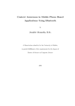
Figure 5.1: Test 1: Noise level in semi-quiet environment. Left picture is 20x gain.
Right picture is with 200x gain
31
CHAPTER 5. TEST AND EVALUATION
Kitchen sink test with a running tap right above the hydrophone, which was placed
in a bucket underneath:
Figure 5.2: Test 2: Running tap. Left picture is 20x gain. Right picture is with 200x
gain
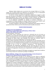
The third test shows the signal strength when dropping a small rock into the water
next to the hydrophone.
Figure 5.3: Test 3: Signal strength - picture is with 20x gain.
We also performed the second and third test, with the running tap and dropping a
rock in water with the hydrophone sensor node and ran the data through Audacity, but
we were unable to get any recognizable sounds from the sample. It might be because
the sample rate is too low, the signal too weak or it might be due to self-noise in the system or all three. The most common cause of self-noise is ground-loops which manifest
themselves as a constant 50 Hz tone that doesn’t vary with volume. In the screen dump
from Audacity (see below) a snippet from a test3 sample can be seen, after removal of
line breaks from the file and a normalize of the signal:
32
CHAPTER 5. TEST AND EVALUATION
Figure 5.4: Screendump from Audacity
At this point in time it would have been really good to be able to substitute the self
made hydrophone for a professional one, in order to eliminate some of these problems.
We are quite sure the hydrophone works, as seen when using the Arduino, but the
Arduino transfers the data through USB, which is significantly faster than the current
sample rate of the SunSPOT. With a lower sample rate we lose a lot of data. With a
professional hydrophone at hand, we could at least have aligned the samples to find a
baseline.
Once the professional hydrophone is available, it could also be very interesting to do
some serious power consumption tests for the system. These tests would prove the
basis for a recalculation of the duty cycle. If we in any way could reduce the power
consumption in run time and combine it with a bigger battery pack, we might have the
possibility to wake up more often to sample.
33
Chapter 6
Conclusion
In this project we have explored the possibility of building and deploying a hydrophone
equipped sensor network mote and we have designed and implemented a working prototype of a SunSPOT based mote. Unfortunately we ran out of time while debugging
the results of the tests conducted with the self made hydrophone. A minimum requirement is a faster analog-to-digital conversion chip, if the SunSPOTs are to keep up with
the sample rate of the hydrophone. Also a better and stronger professional hydrophone
is needed in order to establish the actual performance of the system.
We believe it is feasible to build the designed system despite the problems we have
experienced with our prototype, but it will require a serious effort to obtain the needed
duty cycle with the limited battery capacity to meet the deployment criteria. Also it
will require a detailed plan for several longer field-tests before the actual deployment.
Underwater wireless sensor networks does provide a number of advantages and benefits for aquatic applications, but the design and implementation calls for meticulous
ground work and demands the utmost of the sensor nodes limited and constrained
hardware.
34
Bibliography
[1] An introduction to underwater acoustics: principles and applications, Xavier Lurton, Springer 2003
[2] The Past, Present and Future of Underwater Acoustic Signal Processing, José M. F.
Moura, Carnegie Mellon University, IEEE Signal Processing Magazine, July 1998.
[3] Sensor Networking in Aquatic Environments - Experiences and New Challenges,
ThiemoVoigt et al, Second IEEE International Workshop on Practical Issues in
Building Sensor Network Applications, 15-18 Oct 2007, Dublin, Ireland.
[4] Battery Lifetime estimation and optimization for underwater sensor networks,
Raja Jurdak, Cristina Videira Lopes and Pierre Baldi, University of California,
Wiley-Interscience.
[5] Monitoring in a High-Arctic Environment: Some lessons from MANA, Marcus
Chang and Philippe Bonnet, 2009.
[6] Autonomous Hydrophones at NOAA/OSU and a New Seafloor Sentry System for
Real-time Detection of Acoustic Events, H. Matsumoto et al. IEEE OCEANS 2006.
[7] Challenges: Building Scalable Mobile Underwater Wireless Sensor Networks for
Aquatic Applications, Jun-Hong Cui, ACM 2007
[8] An Underwater Network Testbed: Design, Implementation and Measurement,
Zheng Peng et al, ACM 2007
[9] Fidelity and Yield in a Volcano Monitoring Sensor Network, Georff Werner-Allen
et al.
[10] SunSPOT Developers Guide, Sun Microsystems, Sun Labs, August 2008.
[11] SunSPOT Owners Manual, Sun Microsystems, Sun Labs, August 2008.
[12] SunSPOT Theory of Operation, Sun Microsystems, Sun Labs, August 2008.
[13] Arch Rock IPSerial Node Product Datasheet
[14] User Manual for Aquarian H2A hydrophone
35
BIBLIOGRAPHY
BIBLIOGRAPHY
[15] Datasheet for RESON TC4032 hydrophone
[16] Datasheet for Brüel and Kjær 8103 hydrophone
[17] User manual for Digisnap 2100
[18] ChipCon CC2420 SmartRF datasheet
36
Appendix A
Source code
A.1
Arduino code
// The Arduino code .
# d e f i n e ANALOG IN 0
void setup ( ) {
S e r i a l . begin ( 9 6 0 0 ) ;
}
void loop ( ) {
i n t v a l = analogRead (ANALOG IN ) ;
S e r i a l . p r i n t ( 0 x f f , BYTE ) ;
S e r i a l . p r i n t ( ( v a l >> 8 ) & 0 x f f , BYTE ) ;
S e r i a l . p r i n t ( v a l & 0 x f f , BYTE ) ;
}
37
A.2. PROCESSING CODE
A.2
APPENDIX A. SOURCE CODE
Processing code
/∗
∗ Oscilloscope
∗ Gives a v i s u a l r e n d e r i n g o f analog pin 0 i n r e a l t i m e .
∗
∗ This p r o j e c t i s p a r t o f Accrochages
∗ See h t t p :// a c c r o c h a g e s . drone . ws
∗
∗ ( c ) 2008 S o f i a n Audry ( i n f o @ s o f i a n a u d r y . com )
∗
∗ Modified by S i d s e l J e n s e n t o save data t o f i l e
∗/
import p r o c e s s i n g . s e r i a l . ∗ ;
P r i n t W r i t e r output ;
S e r i a l p o r t ; // C r e a t e o b j e c t from S e r i a l c l a s s
i n t val ;
// Data r e c e i v e d from t h e s e r i a l p o r t
i n t [ ] values ;
void setup ( )
{
size (640 , 480);
// Open t h e p o r t t h a t t h e board i s connected t o and use t h e same speed ( 9 6 0 0 bps )
p o r t = new S e r i a l ( t h i s , S e r i a l . l i s t ( ) [ 1 ] , 9 6 0 0 ) ;
v a l u e s = new i n t [ width ] ;
smooth ( ) ;
output = c r e a t e W r i t e r ( ” output microphone . t x t ” ) ;
}
i n t getY ( i n t v a l ) {
return ( i n t ) ( val / 1023.0 f ∗ height ) − 1 ;
}
void draw ( )
{
while ( p o r t . a v a i l a b l e ( ) >= 3 ) {
i f ( p o r t . read ( ) == 0 x f f ) {
v a l = ( p o r t . read ( ) << 8 ) | ( p o r t . read ( ) ) ;
output . p r i n t l n ( v a l + ”\n ” ) ;
}
}
f o r ( i n t i = 0 ; i <width −1; i ++)
values [ i ] = values [ i + 1 ] ;
v a l u e s [ width −1] = v a l ;
background ( 0 ) ;
stroke ( 2 5 5 ) ;
f o r ( i n t x = 1 ; x<width ; x ++) {
l i n e ( width−x ,
height −1−getY ( v a l u e s [ x − 1 ] ) ,
width−1−x , height −1−getY ( v a l u e s [ x ] ) ) ;
}
}
38
A.2. PROCESSING CODE
APPENDIX A. SOURCE CODE
void keyPressed ( )
{
i f ( key == ’ s ’ ) {
output . f l u s h ( ) ; // Write t h e remaining data
output . c l o s e ( ) ; // F i n i s h t h e f i l e
e x i t ( ) ; // Stop t h e program
}
}
39
A.3. HYDROPHONESPOT CODE
A.3
APPENDIX A. SOURCE CODE
HydrophoneSPOT code
/∗
∗ StartApplication . java
∗
∗ S i d s e l J e n s e n <purps@diku . dk>
∗ HydrophoneSPOT app
∗/
package org . sunspotworld ;
import
import
import
import
import
import
import
import
import
import
import
import
import
com . sun . s po t . p e r i p h e r a l . Spot ;
com . sun . s po t . sensorboard . EDemoBoard ;
com . sun . s po t . sensorboard . p e r i p h e r a l . I S w i t c h ;
com . sun . s po t . sensorboard . p e r i p h e r a l . ITriColorLED ;
com . sun . s po t . p e r i p h e r a l . r a d i o . RadioFactory ;
com . sun . s po t . p e r i p h e r a l . r a d i o . IRadioPolicyManager ;
com . sun . s po t . i o . j2me . r a d i o s t r e a m . ∗ ;
com . sun . s po t . i o . j2me . radiogram . ∗ ;
com . sun . s po t . p e r i p h e r a l . I B a t t e r y ;
com . sun . s po t . sensorboard . hardware . ADT7411 ;
com . sun . s po t . sensorboard . i o . I S c a l a r I n p u t ;
com . sun . s po t . sensorboard . p e r i p h e r a l . LEDColor ;
com . sun . s po t . u t i l . ∗ ;
import
import
import
import
java . io . ∗ ;
javax . microedition . io . ∗ ;
j a v a x . m i c r o e d i t i o n . m i d l e t . MIDlet ;
j a v a x . m i c r o e d i t i o n . m i d l e t . MIDletStateChangeException ;
import
import
import
import
import
import
j a v a x . m i c r o e d i t i o n . rms . I n v a l i d R e c o r d I D E x c e p t i o n ;
j a v a x . m i c r o e d i t i o n . rms . RecordStore ;
j a v a x . m i c r o e d i t i o n . rms . R e c o r d S t o r e E x c e p t i o n ;
j a v a x . m i c r o e d i t i o n . rms . R e c o r d S t o r e F u l l E x c e p t i o n ;
j a v a x . m i c r o e d i t i o n . rms . RecordStoreNotFoundException ;
j a v a x . m i c r o e d i t i o n . rms . RecordStoreNotOpenException ;
/∗∗
∗ The startApp method o f t h i s c l a s s i s c a l l e d by t h e VM t o s t a r t t h e
∗ application .
∗
∗ The m a n i f e s t s p e c i f i e s t h i s c l a s s as MIDlet −1, which means i t w i l l
∗ be s e l e c t e d f o r e x e c u t i o n .
∗/
p u b l i c c l a s s S t a r t A p p l i c a t i o n extends MIDlet {
public
public
public
public
public
static
static
static
static
static
final
final
final
final
final
byte
byte
byte
int
int
ADC REG
SINGLE CHANNEL
AVERAGING OFF
SAMPLE PERIOD
SAMPLE RATE
40
=
=
=
=
=
( byte ) 0 x19 ;
( byte ) 0 x10 ;
( byte ) 0 x20 ;
30;
// how many seconds
7 0 0 0 ; // a t 7k r a t e
A.3. HYDROPHONESPOT CODE
public s t a t i c f i n a l int
APPENDIX A. SOURCE CODE
NO SAMPLES
= SAMPLE PERIOD∗SAMPLE RATE ;
p r i v a t e S t r i n g message = ”empty ” ;
p r i v a t e S t r i n g BSAddr = ” 0 0 1 4 . 4 F01 . 0 0 0 0 . 1 0 C2 ” ;
// p r i v a t e DataInputStream i n = n u l l ;
// p r i v a t e DataOutputStream out = n u l l ;
p r i v a t e DatagramConnection dgBS = n u l l ;
p r i v a t e boolean t a l k e d t o B S = f a l s e ;
RecordStore rms ;
i n t recordStoreIndex = 0 ;
// t o measure b a t t e r y l e v e l
I B a t t e r y B a t t e r y = Spot . g e t I n s t a n c e ( ) . g e t P o w e r C o n t r o l l e r ( ) . g e t B a t t e r y ( ) ;
// t o use t h e Leds
p r i v a t e ITriColorLED [ ] l e d s = EDemoBoard . g e t I n s t a n c e ( ) . getLEDs ( ) ;
I S w i t c h sw1 = EDemoBoard . g e t I n s t a n c e ( ) . g e t S w i t c h e s ( ) [ EDemoBoard . SW1 ] ;
I S w i t c h sw2 = EDemoBoard . g e t I n s t a n c e ( ) . g e t S w i t c h e s ( ) [ EDemoBoard . SW2 ] ;
I S c a l a r I n p u t a n al o gI n = EDemoBoard . g e t I n s t a n c e ( ) . g e t S c a l a r I n p u t s ( ) [ EDemoBoard . A0 ] ; // can use
// s t o r e about one second o f data
p r i v a t e i n t v a l u e s [ ] = new i n t [ 7 0 0 0 ] ;
p u b l i c void connect2GW ( ) {
try {
while ( t a l k e d t o B S == f a l s e ) {
System . out . p r i n t l n ( ”No c o n t a c t t o GW − e s t a b l i s h c o n n e c t i o n ” ) ;
i f ( dgBS == n u l l ) dgBS =
( DatagramConnection ) Connector . open ( ” radiogram ://”+ BSAddr + ” : 3 7 ” ) ;
Datagram dg = dgBS . newDatagram ( dgBS . getMaximumLength ( ) ) ;
sendData ( ”SPOT s i g n i n g i n ” ) ;
System . out . p r i n t l n ( ” Sent : SPOT s i g n i n g i n t o b a s e s t a t i o n ” ) ;
Utils . sleep ( 5 0 0 0 ) ;
dgBS . r e c e i v e ( dg ) ; // hang here wait f o r ACK from BS
message = dg . readUTF ( ) ;
System . out . p r i n t l n ( ” Received : ” + message ) ;
while ( ! message . e q u a l s I g n o r e C a s e ( ”ACK” ) ) {
//s ålænge den kun modtager tomme beskeder s å hæng her !
Utils . sleep ( 1 0 0 0 ) ;
dgBS . r e c e i v e ( dg ) ; // hang here wait f o r ACK from BS
message = dg . readUTF ( ) ;
System . out . p r i n t l n ( ” While loop r e c e i v e d : ” + message ) ;
}
i f ( message . e q u a l s I g n o r e C a s e ( ”ACK” ) ) {
System . out . p r i n t l n ( ” Received : ” + message + ” from GW” ) ;
41
A.3. HYDROPHONESPOT CODE
APPENDIX A. SOURCE CODE
talkedtoBS = true ;
} else {
System . out . p r i n t l n ( ” Wrong i n i t i a l i s a t i o n msg from b a s e s t a t i o n ” ) ;
}
}
} c a t c h ( IOException e ) {
System . out . p r i n t l n ( ”No r o u t e t o 0 0 1 4 . 4 F01 . 0 0 0 0 . 1 0 C2 ” ) ;
} finally {
}
}
synchronized p u b l i c void sendData ( S t r i n g m) {
try {
Datagram dgreply = dgBS . newDatagram ( dgBS . getMaximumLength ( ) ) ;
dgreply . writeUTF (m) ;
dgBS . send ( dgreply ) ;
} c a t c h ( IOException ex ) {
ex . p r i n t S t a c k T r a c e ( ) ;
}
}
p u b l i c void startSW1WatchThread ( ) {
new Thread ( ) {
p u b l i c void run ( ) {
while ( t r u e ) {
sw1 . waitForChange ( ) ;
i f ( sw1 . i s C l o s e d ( ) ) {
sw1Closed ( ) ;
} else {
sw1Opened ( ) ;
}
}
}
}. start ( ) ;
}
p u b l i c void startSW2WatchThread ( ) {
new Thread ( ) {
p u b l i c void run ( ) {
while ( t r u e ) {
sw2 . waitForChange ( ) ;
i f ( sw2 . i s C l o s e d ( ) ) {
sw2Closed ( ) ;
} else {
sw2Opened ( ) ;
}
}
}
}. start ( ) ;
}
p u b l i c void sw1Opened ( ) {
42
A.3. HYDROPHONESPOT CODE
APPENDIX A. SOURCE CODE
System . out . p r i n t l n ( ” Switch 1 opened . ” ) ;
}
p u b l i c void sw2Opened ( ) {
System . out . p r i n t l n ( ” Switch 2 opened . ” ) ;
}
p u b l i c void sw1Closed ( ) {
System . out . p r i n t l n ( ” Switch 1 c l o s e d . ” ) ;
i f ( ! l e d s [ 0 ] . isOn ( ) ) {
System . out . p r i n t l n ( ” S t a r t sampling data . ” ) ;
l e d s [ 0 ] . s e t C o l o r ( LEDColor .GREEN ) ;
l e d s [ 0 ] . setOn ( ) ;
connect2GW ( ) ;
try {
sample ( ) ;
} c a t c h ( RecordStoreNotOpenException ex ) {
ex . p r i n t S t a c k T r a c e ( ) ;
} c a t c h ( I n v a l i d R e c o r d I D E x c e p t i o n ex ) {
ex . p r i n t S t a c k T r a c e ( ) ;
}
} else {
System . out . p r i n t l n ( ” System i s a l r e a d y sampling ! ” ) ;
}
}
p u b l i c void sw2Closed ( ) {
System . out . p r i n t l n ( ” Switch 2 c l o s e d . ” ) ;
i f ( l e d s [ 0 ] . isOn ( ) ) {
System . out . p r i n t l n ( ” Stop sampling data . ” ) ;
// d i s c o n n e c t from GW
leds [ 0 ] . setOff ( ) ;
} else {
System . out . p r i n t l n ( ” System i s not c u r r e n t l y running ! ” ) ;
}
}
p u b l i c void sample ( ) throws RecordStoreNotOpenException , I n v a l i d R e c o r d I D E x c e p t i o n {
S t r i n g B u f f e r sb = new S t r i n g B u f f e r ( ) ;
S t r i n g msg = ”empty ” ;
i n t i , value = 1 ;
i n t count = 0 ;
byte [ ] outputData = n u l l ;
// c u r r e n t main loop − read ˜ 1 s e c o f data and p r i n t s i t out
System . out . p r i n t l n ( ” Saving v a l u e s t o RecordStore . . . \ n ” ) ;
while ( t r u e ) {
f o r ( i = 1 ; i < 7 0 0 0 ; i ++) {
try {
//add value t o RecordStore
value = a na l og I n . getValue ( ) ;
43
A.3. HYDROPHONESPOT CODE
APPENDIX A. SOURCE CODE
Utils . sleep ( 5 0 0 0 ) ;
msg = I n t e g e r . t o S t r i n g ( value ) ;
try {
v a l u e s [ i ] = rms . addRecord ( msg . g e t B y t e s ( ) , 0 , msg . g e t B y t e s ( ) . l e n g t h ) ;
} c a t c h ( R e c o r d S t o r e E x c e p t i o n ex ) {
ex . p r i n t S t a c k T r a c e ( ) ;
}
// v a l u e s [ i ] = an a lo g In . getValue ( ) ;
count ++;
System . out . p r i n t l n ( count + ” ” + value ) ;
// pack data i n bundles o f 15 samples and send
try {
outputData = rms . getRecord ( i ) ;
} c a t c h ( R e c o r d S t o r e E x c e p t i o n ex ) {
ex . p r i n t S t a c k T r a c e ( ) ;
}
i f ( i == 6 9 9 9 ) {
S t r i n g data = new S t r i n g ( outputData ) ;
sb . append ( data + ” EOF ” ) ;
} else {
S t r i n g data2 = new S t r i n g ( outputData ) ;
sb . append ( data2 + ” ” ) ;
}
i f ( ( i > 0 ) && ( ( i % 1 5 ) == 0 ) ) {
// f l a s h l e d 2 while sending data
l e d s [ 1 ] . s e t C o l o r ( LEDColor . RED ) ;
l e d s [ 1 ] . setOn ( ) ;
msg = sb . t o S t r i n g ( ) ;
System . out . p r i n t l n ( ” msg t o GW: ” + i + ” ” + msg ) ;
sendData ( msg ) ;
sb . d e l e t e ( 0 , sb . l e n g t h ( ) ) ;
leds [ 1 ] . setOff ( ) ;
}
} c a t c h ( IOException ex ) {
ex . p r i n t S t a c k T r a c e ( ) ;
}
}
try {
// make d e l i m i t e r between samples
rms . addRecord ( ” f i n i s h ” . g e t B y t e s ( ) , 0 , ” f i n i s h ” . g e t B y t e s ( ) . l e n g t h ) ;
} c a t c h ( R e c o r d S t o r e E x c e p t i o n ex ) {
ex . p r i n t S t a c k T r a c e ( ) ;
}
// s t a t u s on t h e sp o t
System . out . p r i n t l n ( ” Free Memory l e f t on SPOT : ” + Runtime . getRuntime ( ) . freeMemory ( )
44
A.3. HYDROPHONESPOT CODE
APPENDIX A. SOURCE CODE
System . out . p r i n t l n ( ” The c u r r e n t b a t t e r y l v l i s : ” + B a t t e r y . g e t B a t t e r y L e v e l ( ) + ”%”);
System . out . p r i n t l n ( ” The remaining c a p a c i t y i n mwh i s : ” + B a t t e r y . g e t A v a i l a b l e C a p a c i t y ( ) ) ;
count = 0 ;
i = 0;
// send remaining data t o GW
msg = sb . t o S t r i n g ( ) ;
System . out . p r i n t l n ( ” msg t o GW: ” + msg ) ;
sendData ( msg ) ;
// c l o s e t h e r e c o r d S t o r e
// t r y {
//
rms . c l o s e R e c o r d S t o r e ( ) ;
//} c a t c h ( R e c o r d S t o r e E x c e p t i o n ex ) {
//
ex . p r i n t S t a c k T r a c e ( ) ;
//}
}
}
p r o t e c t e d void startApp ( ) throws MIDletStateChangeException {
System . out . p r i n t l n ( ” Hello , world ” ) ;
new B o o t l o a d e r L i s t e n e r ( ) . s t a r t ( ) ;
// monitor t h e USB ( i f connected ) and r e c o g n i z e comman
long ourAddr = RadioFactory . getRadioPolicyManager ( ) . getIEEEAddress ( ) ;
System . out . p r i n t l n ( ” Our r a d i o address = ” + IEEEAddress . toDottedHex ( ourAddr ) ) ;
System . out . p r i n t l n ( ” The c u r r e n t b a t t e r y l v l i s : ” + B a t t e r y . g e t B a t t e r y L e v e l ( ) + ”%”);
System . out . p r i n t l n ( ” The remaining c a p a c i t y i n mwh i s : ” + B a t t e r y . g e t A v a i l a b l e C a p a c i t y ( ) ) ;
//ADT7411 adc = ( ADT7411 ) ( EDemoBoard . g e t I n s t a n c e ( ) . getADC ( ) ) ;
// e n a b l e s i n g l e channel mode
//adc . w r i t e (ADC REG, ( byte ) ( SINGLE CHANNEL + AVERAGING OFF + an a lo g In . g e t I n d e x ( ) . t o I n t e g e r
//do t h e heavy s t u f f b e f o r e we s t a r t sampling t o keep up s a m p l e r a t e
// c r e a t e or open RecordStore
System . out . p r i n t l n ( ” D e l e t i n g old RecordStore . . . ( p l e a s e wait ) \ n ” ) ;
try {
// i f r e c o r d s t o r e e x i s t s − then d e l e t e i t so we have room f o r new samples
try {
i f ( RecordStore . l i s t R e c o r d S t o r e s ( ) ! = n u l l ) {
RecordStore . d e l e t e R e c o r d S t o r e ( ” SampleData ” ) ;
System . out . p r i n t l n ( ” Done ! ” ) ;
}
} c a t c h ( R e c o r d S t o r e E x c e p t i o n ex ) {
ex . p r i n t S t a c k T r a c e ( ) ;
}
System . out . p r i n t l n ( ” C r e a t i n g new RecordStore . . . ( p l e a s e wait ) \ n ” ) ;
rms = RecordStore . openRecordStore ( ” SampleData ” , t r u e ) ;
System . out . p r i n t l n ( ” Done ! ” ) ;
} c a t c h ( R e c o r d S t o r e E x c e p t i o n ex ) {
ex . p r i n t S t a c k T r a c e ( ) ;
}
45
A.3. HYDROPHONESPOT CODE
APPENDIX A. SOURCE CODE
// s t a r t program by p r e s s i n g sw1
startSW1WatchThread ( ) ;
// st op program by p r e s s i n g sw2
startSW2WatchThread ( ) ;
System . out . p r i n t l n ( ” P r e s s l e f t button t o s t a r t sampling . . . ” ) ;
// sync time with h o s t
// a f t e r l a s t data s e n t − send b a t t e r y and time s t a t u s
// go i n t o deep s l e e p /duty c y c l e
}
p r o t e c t e d void pauseApp ( ) {
// This i s not c u r r e n t l y c a l l e d by t h e Squawk VM
}
/∗∗
∗ C a l l e d i f t h e MIDlet i s t e r m i n a t e d by t h e system .
∗ I . e . i f startApp throws any e x c e p t i o n o t h e r than MIDletStateChangeException ,
∗ i f t h e i s o l a t e running t h e MIDlet i s k i l l e d with I s o l a t e . e x i t ( ) , or
∗ i f VM. stopVM ( ) i s c a l l e d .
∗
∗ I t i s not c a l l e d i f MIDlet . n o t i f y D e s t r o y e d ( ) was c a l l e d .
∗
∗ @param u n c o n d i t i o n a l I f t r u e when t h i s method i s c a l l e d , t h e MIDlet must
∗
cleanup and r e l e a s e a l l r e s o u r c e s . I f f a l s e t h e MIDlet may throw
∗
MIDletStateChangeException t o i n d i c a t e i t does not want t o be destroyed
∗
a t t h i s time .
∗/
p r o t e c t e d void destroyApp ( boolean u n c o n d i t i o n a l ) throws MIDletStateChangeException {
f o r ( i n t i = 0 ; i < 8 ; i ++) {
leds [ i ] . setOff ( ) ;
}
}
}
46
A.4. HYDROPHONEHOST CODE
A.4
APPENDIX A. SOURCE CODE
HydrophoneHOST code
/∗
∗ SunSpotHostApplication . j a v a
∗
∗ S i d s e l J e n s e n <purps@diku . dk>
∗ HydrophoneHOST app
∗/
package org . sunspotworld ;
import
import
import
import
import
com . sun . s po t . p e r i p h e r a l . r a d i o . RadioFactory ;
com . sun . s po t . p e r i p h e r a l . r a d i o . IRadioPolicyManager ;
com . sun . s po t . i o . j2me . r a d i o s t r e a m . ∗ ;
com . sun . s po t . i o . j2me . radiogram . ∗ ;
com . sun . s po t . u t i l . IEEEAddress ;
import
import
import
import
import
import
com . sun . s po t . u t i l . U t i l s ;
java . io . ∗ ;
j a v a . t e x t . DateFormat ;
j a v a . u t i l . l o g g i n g . Level ;
j a v a . u t i l . l o g g i n g . Logger ;
javax . microedition . io . ∗ ;
/∗∗
∗ Sample Sun SPOT h o s t a p p l i c a t i o n
∗/
p u b l i c c l a s s SunSpotHostApplication {
private s t a t i c final int
RADIOGRAMPORT
p r i v a t e s t a t i c f i n a l S t r i n g SPOTADDR
= 37;
= ” 0 0 1 4 . 4 F01 . 0 0 0 0 . 1 A32 ” ;
// p r i v a t e DatagramConnection dgBConn = n u l l ;
p r i v a t e S t r i n g message = ”empty ” ;
p r i v a t e RadiogramConnection conn , conn2 = n u l l ;
p r i v a t e Datagram dgreply = n u l l ;
p r i v a t e Datagram data = n u l l ;
p u b l i c void c o n n e c t 2 s p o t ( ) {
try {
conn = ( RadiogramConnection ) Connector . open ( ” radiogram : / / 0 0 1 4 . 4 F01 . 0 0 0 0 . 1 A32 : 3 7 ” ) ;
dgreply = conn . newDatagram ( conn . getMaximumLength ( ) ) ;
System . out . p r i n t l n ( ” Awaiting c o n n e c t i o n attempt from SPOT ” ) ;
conn . r e c e i v e ( dgreply ) ;
message = dgreply . readUTF ( ) ;
System . out . p r i n t l n ( ” Received : ” + message ) ;
i f ( message . e q u a l s I g n o r e C a s e ( ”SPOT s i g n i n g i n ” ) ) {
Utils . sleep ( 5 0 0 0 ) ;
47
A.4. HYDROPHONEHOST CODE
APPENDIX A. SOURCE CODE
data = conn . newDatagram ( conn . getMaximumLength ( ) ) ;
data . writeUTF ( ”ACK” ) ;
conn . send ( data ) ;
System . out . p r i n t l n ( ” Sent ACK t o c l i e n t ” ) ;
message = ”empty ” ;
//dgreply = n u l l ;
} else {
System . out . p r i n t l n ( ” Something went wrong ! ” ) ;
}
} c a t c h ( IOException e ) {
System . out . p r i n t l n ( ”No c o n n e c t i o n ” ) ;
} finally {
//conn . c l o s e ( ) ;
}
}
p u b l i c S t r i n g lastWord ( S t r i n g s ) {
S t r i n g lastWord = ” ” ;
i n t spaceIndex
i f ( spaceIndex
lastWord =
} else {
lastWord =
}
= s . indexOf ( ’
== −1) {
s;
’);
s . substring ( s . lastIndexOf ( ’
’) + 1);
//System . out . p r i n t l n ( ” L a s t word i n message i s : ” + lastWord ) ;
r e t u r n lastWord ;
}
/∗∗
∗ P r i n t out our r a d i o address .
∗/
p u b l i c void run ( ) throws FileNotFoundException , Ex ce pti on {
long ourAddr = RadioFactory . getRadioPolicyManager ( ) . getIEEEAddress ( ) ;
System . out . p r i n t l n ( ” Our r a d i o address = ” + IEEEAddress . toDottedHex ( ourAddr ) ) ;
// i n i t i a l i z a t i o n o f c o n n e c t i o n v a r i a b l e s f o r radiogram communication
// wait f o r SPOT t o c o n t a c t us . . .
connect2spot ( ) ;
System . out . p r i n t l n ( ” P o r t ” + RADIOGRAMPORT + ” i s open and l i s t e n i n g f o r a c l i e n t .
System . out . p r i n t l n ( ” Radiogram c o n n e c t i o n i s e s t a b l i s h e d with Free−Range SPOT . . . ” )
System . out . p r i n t l n ( ” Waiting f o r incoming data . . .
\n ” ) ;
// Define t h e date/time format t o use
DateFormat format = DateFormat . g e t T i m e I n s t a n c e ( ) ;
// V a r i a b l e s t o w r i t e 2 a f i l e
FileOutputStream
File2OutputData = n u l l ;
PrintStream
MyOutputFile
= null ;
File2OutputData = new FileOutputStream ( ” HydrophoneValuesFromSPOT . csv ” ) ;
MyOutputFile
= new P r i n t S t r e a m ( File2OutputData ) ;
48
A.4. HYDROPHONEHOST CODE
APPENDIX A. SOURCE CODE
// S t r i n g t o save t h e data t o s t o r e on t h e f i l e
S t r i n g Data2Write ;
S t r i n g data ;
i n t count = 0 ;
S t r i n g B u f f e r incomingdata = new S t r i n g B u f f e r ( ) ;
// await incoming data
while ( t r u e ) {
try {
// Read data r e c e i v e d over t h e r a d i o
Utils . sleep ( 5 0 ) ;
conn . r e c e i v e ( dgreply ) ;
S t r i n g addr = dgreply . getAddress ( ) ; // read sender ’ s Id
System . out . p r i n t l n ( ” Data has been r e c e i v e d . . .
”);
//pa rse data r e c e i v e d
data = dgreply . readUTF ( ) ;
incomingdata . append ( data + ”\n ” ) ;
Data2Write = incomingdata . t o S t r i n g ( ) ;
System . out . p r i n t l n ( ” Received from SPOT : ” + count + ” ” + data ) ;
count ++;
// save hydrophone−data t o f i l e
// have we reached EOF? i f so save t o f i l e
i f ( lastWord ( data ) . e q u a l s I g n o r e C a s e ( ”EOF ” ) ) {
MyOutputFile . p r i n t l n ( Data2Write ) ;
System . out . p r i n t l n ( ” Data has been w r i t t e n i n f i l e
// r e s e t t h e s t r i n g b u f f e r
incomingdata . d e l e t e ( 0 , incomingdata . l e n g t h ( ) ) ;
}
} c a t c h ( E xce pt ion e ) {
System . e r r . p r i n t l n ( ” Caught ” + e +
throw e ;
}
...
\n ” ) ;
” while reading s e n s o r samples . ” ) ;
}
}
/∗∗
∗ S t a r t up t h e h o s t a p p l i c a t i o n .
∗
∗ @param a r g s any command l i n e arguments
∗/
p u b l i c s t a t i c void main ( S t r i n g [ ] a r g s ) throws Ex ce pti on {
try {
SunSpotHostApplication app = new SunSpotHostApplication ( ) ;
app . run ( ) ;
} c a t c h ( FileNotFoundException ex ) {
Logger . getLogger ( SunSpotHostApplication . c l a s s . getName ( ) ) . l o g ( Level . SEVERE , n u l l , ex ) ;
49
A.4. HYDROPHONEHOST CODE
APPENDIX A. SOURCE CODE
}
}
}
50