Download Multi-scale edge detection wizard (T44a)

INTREPID User Manual
Library | Help | Top
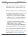
Multi-scale edge detection wizard (T44a)
1
| Back |
Multi-scale edge detection wizard (T44a)
Top
INTREPID’s unique multiscale edge analysis tool finds local maxima points of the
total horizontal derivative for many upward continuations of data.
Stating the obvious, if your survey covers a small prospect, the longest wavelength
that can be captured in your survey area is half its minimum extent, without any
alias effects. So, when it comes to detecting deeper faults and contacts, by a process of
upwards continuation, there is no point continuing your survey data even to this
minimum width extent, as no deeper feature can be found in the data.
By way of 2 examples,
a. If you have a sound regional gravity grid with good signal content, either from an
airborne survey at better than 1 km line spacing, or a ground based survey(s) and you
wish to make a “sounding” down to the Moho, then you need to have a spatial extent
of say 100 kms in both directions as a minimum.
b. If you are looking for faults/dykes in a near surface coal deposit, and have a ground
based survey that covers around 4 kms square, then the deepest features will report
to about 1 km
At V4.5 onwards, Tensor grids are supported with the following comments.
Ordinary Full tensor gravity gradient tensor grids, as created by the Intrepid
gridding tool, have 2 edge picking options. The Falcon tensor grids remains to
finalized, as the measured signal is not compatiable with the general
requirements of the technology - the maximum horizontal curvature anomaly (
Txy,Tuv) of the Falcon, represents a departure from a perfect spherical body, as
opposed to the maximum horizontal gradien ( Tzx,Tyz), as used traditionally,
repesents contact edges.
As well as calculating the maxima, this tool can
•
Calculate Euler depth estimates for all points
•
Associate neighbouring points into ‘worms’ (strings) that define the edges
•
Using linear regression, create a straight line that characterises each worm.
•
New 3D surface clustering, to create 3 csv files suitable for import into
Geomodeller, to locate the main contacts in a 3D model space.
•
Create a registered Tiff image of a reduction of all the WORMS, emphasing the
ones with more expression at depth.
The tool uses potential field geophysical data to provide an excellent starting point for
an interpretation of structural geology. See References for further information about
these techniques,
The Multi-scale edge detection wizard creates many upward continuation grids. You
can use the calculated lines to analyse strike distributions for structural units at
depth. The tool is suitable for regional areas as large as Cratons or State
compilations at high resolution.
This technique was originally developed for standard scalar gravity data. You can
use the tool with magnetic data (TMI), but we recommend that you first reduce the
magnetic data to the pole. The extra step of conversion to a monopole via a
pseudogravity transform is also present.(see Spectral domain grid filters tool
(GridFFT) (T40)). The Multi-scale edge detection wizard supports both of these
Library | Help | Top
© 2012 Intrepid Geophysics
| Back |
INTREPID User Manual
Library | Help | Top
Multi-scale edge detection wizard (T44a)
2
| Back |
processes for magnetic data. FTG data processing follows the same workflow in this
tool, including upward continuation, point picking maximum gradients, joining the
points into worms, formation of linears, and now the 3D surface clustering algorithm.
WARNING - Whilst Geodetic grids are supported, you can get into more trouble than
it may be worth. Note, we are upwards continuing, assuming a planar or flat world.
The units of upwards continuation are meters. For the Geodetic case, we internally
make these equivalent decimal degrees to follow your wishes. Also, as the points are
located to form the WORMS, the tolerances are stretched. The output projection of
derived datsets follows from the input grid.
A Lambert Conic Conformal projection is often used when a continental or very large
regional extent is involved.
In this chapter:
How to use this chapter
Overview of the Multi-scale edge detection wizard process
Using the Multi-scale edge detection wizard—overview (interactive only)
Step 1—Specify input dataset, scalar TMI grid example
Step 2—Pre-process and filter
Step 3—Calculate edge points
Step 4—Group edge points into 'worms'
Step 5 - Calculate linears
Step 7—Export results
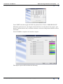
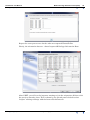
Specifying input and output files
All further options are common to the previous tutorial descriptions. The next
image shows the stacked “worms” for this dataset in the Intrepid Visual tool. The
amplitude field is used to colour code the polylines. The deeper, more important
contacts, are shown in red.
Apply
Exit
Task specification (.job) files
Finding out more about spectral domain operations
Glossary
References
Library | Help | Top
© 2012 Intrepid Geophysics
| Back |
INTREPID User Manual
Library | Help | Top
Multi-scale edge detection wizard (T44a)
3
| Back |
How to use this chapter
Parent topic:
Multi-scale edge
detection wizard
(T44a)
This chapter describes the operation of the Multi-scale edge detection wizard. You
can use the it both interactively and in INTREPID batch processing mode, using
INTREPID task specification (.job) files.
At V5.0 Intrepid, support for GOOGLE protobuf *.task batch files is also available,
and therefore the complete datamodel language is published and distributed by
Intrepid. Initially, this functionality is a straight duplication of the older Intrepid
datamodel technology.
Where needed in this chapter, there are separate Interactive and Task files sections.
Some sections may be marked Interactive only or Task files only.
You can find out how to use the tool and also get background information as follows:
•
For instructions on using the tool interactively see Using the Multi-scale edge
detection wizard—overview (interactive only).
•
For details about task specification (.job) files, see Task specification (.job) files
•
For batch mode instructions, see Creating and using task specification files.
•
For relevant information in other chapters, see Finding out more about spectral
domain operations.
Overview of the Multi-scale edge detection wizard process
Parent topic:
Multi-scale edge
detection wizard
(T44a)
The Multi-scale edge detection wizard process consists of the following steps:
Prepare input dataset
1
Load the input grid dataset (see Specifying the input grid)
2
(Optional) Create subset of input grid dataset (see Specifying a subsection of the
input grid).
3
Transform input grid to the spectral domain using Fast Fourier Transform (FFT),
saving products if required (see Pre FFT grid conditioning and Saving FFT
products ).
4
(Optional) Apply a reduction to the pole filter (see Specifying reduction to pole).
5
Specify upward continuation levels (see Specifying upward continuation levels).
Process data for each continuation level
6
(Optional, for high continuation levels) Rarefy the cell sampling (see Rarefying
cell sampling).
7
Apply the upward continuation filter, producing a filtered grid in the spectral
domain (see "Continuation filters (reference)" in INTREPID spectral domain
operations reference (R14)).
8
Produce total horizontal derivative, X derivative and Y derivative grids (see
"Compound derivative filters" in INTREPID spectral domain operations reference
(R14) and "Single derivative filters" in INTREPID spectral domain operations
reference (R14)) (and keep copies if required—see Saving derivative grids). Note,
as these are measured quantities in a tensor grid, there is no need to calculate
these gradients. In terms of an FTG signal, we use the Tzx and Tyz gradients
components, as these are functionaliy equivalent.
9
Find edge points in the derivative grids (see Step 3—Calculate edge points).
10 (Optional) Save edge points to a line dataset (see Step 3—Calculate edge points)
Library | Help | Top
© 2012 Intrepid Geophysics
| Back |
INTREPID User Manual
Library | Help | Top
Multi-scale edge detection wizard (T44a)
4
| Back |
11 Associate edge points that are close together into ‘worms’ and save to a line
dataset (see Step 4—Group edge points into 'worms').
12 (Optional) Use Euler deconvolution to calculate representative depth of each
worm, assuming that the depth ans Structural Index must be addmissable, and
that a least squares best estimate will do. (see Step 3—Calculate edge points).
13 (Optional) From each worm, use linear regression to calculate a straight line
segment, showing strike and length of the worm. Save this data to a line dataset.
14 Unconditionally, starting from the ‘worms’ database and the deepest predicted
edges, build up by a spatial clustering algorithm, 3D surface points, foliations and
feature radius bounds, from the mean position of the contact. Save this to 3 csv
files, in a format suitable for direct fault network creation within Geomodeller.
15 Supplementary file formats for ArcMap, MapInfo, GoCAD and VRML are also
supported.
Library | Help | Top
© 2012 Intrepid Geophysics
| Back |
INTREPID User Manual
Library | Help | Top
Multi-scale edge detection wizard (T44a)
5
| Back |
Using the Multi-scale edge detection wizard—overview (interactive only)
Parent topic:
Multi-scale edge
detection wizard
(T44a)
This section is an overview of the tool in interactive mode. The first part
demonstrates a standard scalar geophysical grid from the Intrepid\Examples datsets
and jobs distributed with every installation of Intrepid. A second tensor gravity
gradient example is then also described, also using data from the COOKBOOK/tensor
section of the distribution.
For information about batch mode operation, see Creating and using task
specification files.
Interactive
>> To use Multi-scale edge detection wizard with the INTREPID graphic user
interface
1
Choose Multi Scale Edge Detection from the Interpretation menu in the Project
Manager, or use the command worme.exe. INTREPID displays the Multi-scale
edge detection wizard window.
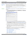
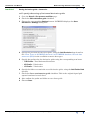
2
If you have previously prepared file specifications and parameter settings for
Multi-scale edge detection wizard, load the corresponding task specification file
using Load Options from the File menu. (See Specifying input and output files for
detailed instructions.) If all of the specifications are correct in this file, go to step
6. If you wish to modify any settings, carry out the following steps as required.
3
Set a folder to receive a range of output products - grids, comma seperated ASCII
files with points, lines etc at each continuation level, and the GIS style
supplementary outputs. If the folder name already exists, eg output, then
output1, output2 etc is choosen as necessary, to make sure a unique output folder
exists for each run.
4
Set the options on each page of the wizard as required. Use the Next and
Previous buttons to move between the windows. See the following sections for
information about options on the individual pages:
Step 1—Specify input dataset, scalar TMI grid example
Step 2—Pre-process and filter
Step 3—Calculate edge points
Step 4—Group edge points into 'worms'
Step 5 - Calculate linears
Step 7—Export results
Also—Specifying input and output files.
5
Library | Help | Top
(When you have finished setting options for the task) If you wish to record the
© 2012 Intrepid Geophysics
| Back |
INTREPID User Manual
Library | Help | Top
Multi-scale edge detection wizard (T44a)
6
| Back |
specifications for this process in a .job file so that you can repeat a similar task
later or for some other reason, use Save Options from the File menu. See
Creating and using task specification files for detailed instructions.
6
(When you are ready to execute the task) In the last page (Supplementary
Outputs), choose Finish. INTREPID executes the Multi-scale edge detection
wizard task.
7
To exit from Multi-scale edge detection wizard, without running the process
choose Exit from the File menu or use the Cancel button.
Step 1—Specify input dataset, scalar TMI grid example
Parent topic:
Multi-scale edge
detection wizard
(T44a)
In this step you can specify:
•
Input grid and band—see Specifying the input grid
•
Subsection of input grid—see Specifying a subsection of the input grid
Specifying the input grid
Parent topic:
Step 1—Specify
input dataset,
scalar TMI grid
example
In this section:
•
Specifying the input grid—interactive
•
Specifying the input grid—batch files
Note: The current version of this tool only supports projected input grids with metres
as distance unit.
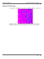
Below is an illustration of a grid that we shall use as a case study in this chapter.
Library | Help | Top
© 2012 Intrepid Geophysics
| Back |
INTREPID User Manual
Library | Help | Top
Interactive
Multi-scale edge detection wizard (T44a)
7
| Back |
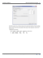
Specifying the input grid—interactive
>> To specify the input grid:
Task files
1
Enter the full path and file name in the Input Grid text box or use the Browse [...]
button to locate it.
2
Select the band you want to process using the Input Band spin box.
3
(If you want to specify a subsection of the input grid dataset) See Specifying a
subsection of the input grid.
Specifying the input grid—batch files
1
PARMS job file syntax
Within the Input_Grid Begin – End block:
•
Use the Input_Grid keyword to specify the full path of the input grid.
•
Use the Input_Band keyword to select the band to be processed.
For example (instead of install_path insert the location of your INTREPID
installation):
Input_Grid Begin
Input_Grid=
install_path\examples\jobs\datasets\mlevel_grid.ers
Input_Band= 0
Input_Grid End
2
PROTOBUF task file syntax
Within the InputGridName sub block:
For Example:
InputGridName {
grid: "../datasets/mlevel_grid.ers";
type: Magnetism;
Band: 1;
mean_elevation: 100;
}
Library | Help | Top
© 2012 Intrepid Geophysics
| Back |
INTREPID User Manual
Library | Help | Top
Multi-scale edge detection wizard (T44a)
8
| Back |
Specifying a subsection of the input grid
Parent topic:
Step 1—Specify
input dataset,
scalar TMI grid
example
In this section:
Interactive
Specifying a subsection of the input grid—interactive
•
Specifying a subsection of the input grid—interactive
•
Specifying a subsection of the input grid—task files
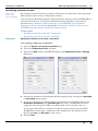
>> To specify a subsection of the input grid:
Task files
1
Go to the Step 1—Specify input dataset page
2
Specify the input grid dataset (see Specifying the input grid).
3
Check the Process a subsection only checkbox.
4
Enter the extents of the subsection in the X (West), X (East), Y (North), Y (South)
text boxes. X (West) and Y (South) contain the lower extent values.
5
(If you want to specify a name for the subsection grid that INTREPID saves)
specify the file name in the Save grid subsection as text box. If you don’t specify
a name, INTREPID uses the default name shown in the text box.
Specifying a subsection of the input grid—task files
1
PARMS job file syntax
Within the Input_Grid Begin – End block, insert a Subset Begin – End block:
•
Use the XUpper, XLower, YUpper, YLower keywords to specify the extents of the
subsection.
•
Use the SubsetGrid keyword to specify the name of the subsection grid that
INTREPID saves.
For example:
Subset Begin
XUpper= 740000.000000
XLower= 752001.000000
YUpper= 8419999.000000
YLower= 8407999.000000
SubsetGrid= subset.ers
Subset End
2
PROTOBUF task file syntax
The formal definition of the subset block syntax in protobuf format follows:
message grid_subset_INT {
// subset support during fft filtering ops
// option to define a box explicitly
optional double XLower
=1; // all default to NULL
optional double XUpper
=2;
optional double YLower
=3;
optional double YUpper
=4;
optional double FFT_BorderPercentExpansion
=5 [ default =120]; // subset border in
percentage
optional string SubsetGridName
=6 [ default = "subset.ers"];
// option to define a square subset in terms of cells, for purpose of a moving window power
spectra
optional int32 NumberCellsForFFTPower = 7 [ default = 32]; // should be power of 2 eg 32,64,128
etc
optional bool AutoPowerSpectrumReporting = 8 [ default = false]; // just dump out power spectra
reports
}
Library | Help | Top
© 2012 Intrepid Geophysics
| Back |
INTREPID User Manual
Library | Help | Top
Multi-scale edge detection wizard (T44a)
9
| Back |
Step 2—Pre-process and filter
Parent topic:
Multi-scale edge
detection wizard
(T44a)
Library | Help | Top
In this step you can specify settings for:
Pre-FFT processing—see Pre FFT grid conditioning
Saving FFT products—see Saving FFT products
Reduction to Pole—see Specifying reduction to pole
Continuation levels—see Specifying upward continuation levels
Rarefying cell sampling—see Rarefying cell sampling
Saving derivative grids for each upward continuation level—see Saving derivative
grids
© 2012 Intrepid Geophysics
| Back |
INTREPID User Manual
Library | Help | Top
Multi-scale edge detection wizard (T44a)
10
| Back |
Pre FFT grid conditioning
Parent topic:
Step 2—Preprocess and filter
You can specify how you want INTREPID to prepare the input grid for Fast Fourier
Transform (FFT) to the spectral domain. This part of the tool reuses much of the
same technology as used in the gfilt tool. In this section:
•
Pre-FFT grid conditioning—explanation
•
Edge damping rolloff filters available
•
Pre-FFT grid conditioning—interactive
•
Pre-FFT grid conditioning—task files
Pre-FFT grid conditioning—explanation
The following table outlines the pre-FFT grid conditioning operations.
Operation
Description
Expanding the grid
INTREPID always expands the grid to dimensions suitable for FFT. You can
specify the minimum width of the border surrounding the data-containing
cells. See "Expanding the data area" in INTREPID spectral domain
operations reference (R14) for an explanation of this stage.
Detrending
INTREPID always detrends the grid. See "Detrending data values" in
INTREPID spectral domain operations reference (R14) for information. The
value you select or assign to the keyword corresponds to the degrees in this
reference topic.
Fill method
After expanding the grid, INTREPID assigns values to the new cells in the
grid using an extrapolation process. You can choose one of two available
methods—Arthur fill algorithm and maximum entropy. See "Estimating
values for data gap cells" in INTREPID spectral domain operations reference
(R14) for details.
Grid edge rolloff
For best results from the FFT, the edges of the grid must be set to zero, but
without sudden changes from the data within the grid. The grid data needs to
‘roll off’ to zero at the edge.
See "Damping of dataset edges before spectral transform" in INTREPID
spectral domain operations reference (R14) for details of this process.
INTREPID has two sets of available edge roll off methods for this tool. See
Edge damping rolloff filters available for details
FFT grid precision
Library | Help | Top
You can specify the precision of the spectral domain grid. See "Data Types in
INTREPID datasets" in INTREPID database, file and data structures (R05)
for the available numeric data types.
© 2012 Intrepid Geophysics
| Back |
INTREPID User Manual
Library | Help | Top
Multi-scale edge detection wizard (T44a)
11
| Back |
Edge damping rolloff filters available
INTREPID has two main roll-off methods, each of which has a number of filters.
Interactive
Method
Description
Filters available
Expanded edge
roll-off
Rolloff operation only on the edges of the
grid. See "Expanded edge rolloff" in
INTREPID spectral domain operations
reference (R14) for an explanation.
Cosine
Linear
Whole window
roll-off
Rolloff operation across the whole grid.
See "Damping of dataset edges before
spectral transform" in INTREPID
spectral domain operations reference
(R14) for an explanation.
Cosine bell
Hanning
Hamming
Blackman
Triangle
Pre-FFT grid conditioning—interactive
>> To specify pre-FFT grid conditioning
Library | Help | Top
1
Go to the Step 2—Pre-process and filter page.
2
Choose the FFT Settings button. INTREPID displays the FFT Settings dialog box.
3
Set the pre-FFT operations parameters as required (see Pre-FFT grid
conditioning—explanation):
•
Width of added border (Expanding the grid), units of percent, so 100% means
no expansion!
•
Degree of trend removal (Detrending)
•
Fill type (Fill method)
•
Grid edge rolloff—Edge damping method
•
Grid edge rolloff—Whole grid damping method
•
FFT Grid precision
4
(If you want to save FFT product grids) Choose Save FFT Products and set your
requirements (see Saving FFT products).
5
Choose Close.
© 2012 Intrepid Geophysics
| Back |
INTREPID User Manual
Library | Help | Top
Task files
Multi-scale edge detection wizard (T44a)
12
| Back |
Pre-FFT grid conditioning—task files
See Pre-FFT grid conditioning—explanation for an explanation of parameters.
1
PARMS job file syntax
Within the UC_Filtering Begin – End block:
•
Include the Pre_FFT_Transform Begin – End block:
•
Specify the minimum width of the expanded grid border. Use the FFT_Border
keyword, assigning the width in input grid distance units.
•
Use the Detrend_Degree keyword to specify this parameter.
•
Specify the method for filling empty cells in the expanded grid. Use the
Fill_type keyword, assigning the name of one of the methods:
•
•
•
Fill method
Value to assign
Linear interpolation (Arthur)
ARTHUR
Maximum entropy
MEM
Specify grid edge rolloff—edge damping method. Use the Rolloff_Type
keyword, assigning the name of one of the methods:
Grid edge roll-off method
Rolloff_Type value
Linear
LINEAR
Cosine
COSINE
No roll-off
NONE
Specify grid edge rolloff—whole window damping method. Use the Window_Type
keyword, assigning the name of one of the methods:
Window roll-off method
Window_Type value
Linear
COSINE_BELL
Cosine
HANNING
Hamming
HAMMING
Blackman
BLACKMAN
Bartlett or Triangular
TRIANGLE
No roll-off
NONE
Specify the precision of the FFT grid. Use the FFT_Grid_Precision keyword,
assigning the name of the data type. See "Data Types in INTREPID datasets" in
INTREPID database, file and data structures (R05) for a list.
Example:
Pre_FFT_Transform Begin
Detrend_Degree= 0
Rolloff_Type= COSINE
Window_Type= None
Fill_Type= ARTHUR
FFT_Grid_Precision= IEEE4ByteComplex
Library | Help | Top
© 2012 Intrepid Geophysics
| Back |
INTREPID User Manual
Library | Help | Top
Multi-scale edge detection wizard (T44a)
13
| Back |
FFT_Border= 120.000000
Pre_FFT_Transform End
2
PROTOBUF syntax
Pre_FFT_Transform {
DetrendDegree: 0;
RolloffType: Cosine_RollOff;
WindowType: NO_Window;
FillType: ARTHUR;
FFT_Grid_Precision: IEEE4ByteComplex;
FFT_Border: 166.667; # minimum padding expansion factor as a
percentage
Number_CPUs: 4;
# multi-threading option
}
Saving FFT products
Parent topic:
Step 2—Preprocess and filter
Multi-scale edge detection wizard allows you to keep copies of the following pre-FFT
and FFT grid processing products:
•
Detrended, expanded and filled input grid dataset
•
Detrended, expanded and filled input grid dataset after edge damping
•
FFT of input grid dataset
See "Saving pre-FFT and FFT grid processing products for later reference" in
INTREPID spectral domain operations reference (R14) for discussion about the
benefits of keeping copies of these products.
In this section:
Interactive
•
Saving FFT products—interactive
•
Saving FFT products—task files
Saving FFT products—interactive
>> To specify FFT product saving and keeping:
Library | Help | Top
1
Go to the Step 2—Pre-process and filter page.
2
Choose FFT Settings. INTREPID displays the FFT Settings dialog box.
3
Choose Save FFT Products. INTREPID displays the Save FFT Products dialog
box.
4
For each of the following pre-FFT and FFT products, as required, check the
checkbox and specify the path and filename that you want to use (or accept the
default filename):
•
Expanded and filled grid (Detrended, expanded and filled input grid dataset)
•
Expanded, filled and damped grid (Detrended, expanded and filled input grid
dataset after edge damping)
•
FFT Grid (FFT of input grid dataset)
© 2012 Intrepid Geophysics
| Back |
INTREPID User Manual
Library | Help | Top
5
Library | Help | Top
Multi-scale edge detection wizard (T44a)
14
| Back |
Choose Close.
© 2012 Intrepid Geophysics
| Back |
INTREPID User Manual
Library | Help | Top
Task files
Multi-scale edge detection wizard (T44a)
15
| Back |
Saving FFT products—task files
Within the Pre_FFT_Transform Begin – End block (in the UC_Filtering
Begin – End block):
Library | Help | Top
•
Specify the path and filename of the detrended, expanded and filled input grid
dataset. Use the Expanded_Grid_Path keyword, assigning the full path and file
name for the dataset. Example:
Expanded_Grid_Path =
C:\Datasets\mscale_edge\output\ExpandedGrid.ers
•
Specify the path and filename of the detrended, expanded and filled input grid
dataset after edge damping. Use the Windowed_Grid_Path keyword, assigning
the full path and file name for the dataset. Example
Windowed_Grid_Path =
C:\Datasets\mscale_edge\output\WindowedGrid.ers
•
Specify the path and filename of the FFT of input grid dataset. Use the
FFT_Grid_Path keyword, assigning the full path and file name for the dataset.
Example:
FFT_Grid_Path =
C:\Datasets\mscale_edge\output\FFTGrid.ers
© 2012 Intrepid Geophysics
| Back |
INTREPID User Manual
Library | Help | Top
Multi-scale edge detection wizard (T44a)
16
| Back |
Specifying reduction to pole
Parent topic:
Step 2—Preprocess and filter
We strongly recommend that you apply a reduction to the pole filter to the input grid.
This improves the accuracy of edge point location.
You can specify the Earth magnetic field parameters directly or direct INTREPID to
calculate them for you. For general information about this filter and required
parameters see "Reduction filters (reference)" in INTREPID spectral domain
operations reference (R14) and, specifically, "Reduction to the Pole (reference)" in
INTREPID spectral domain operations reference (R14).
In this section:
Interactive
•
Specifying reduction to the pole—interactive
•
Specifying reduction to the pole—task files
Specifying reduction to the pole—interactive
>> To specify reduction to the pole:
1
Go to the Step 2—Pre-process and filter page
2
Check the Reduction to Pole checkbox.
3
Choose the IGRF button. INTREPID displays the Reduction to Pole—Settings
dialog box.
4
Specify the method of calculating the Earth magnetic field, selecting the Specified
or Calculated option button.
5
(If you are specifying the Earth magnetic field) Enter the required values in the
Inclination, Declination and Field Strength text boxes. INTREPID calculates
suggested values from the IGRF and shows them in the text boxes for you.
(If you want INTREPID to calculate the Earth magnetic field from the IGRF)
INTREPID calculates the coordinates of the mid point of the dataset for you.
Specify the Date and Elevation of the survey.
6
Library | Help | Top
Choose Close.
© 2012 Intrepid Geophysics
| Back |
INTREPID User Manual
Library | Help | Top
Task files
Multi-scale edge detection wizard (T44a)
17
| Back |
Specifying reduction to the pole—task files
1
PARMS job file syntax
Within the UC_Filtering Begin – End block:
•
Include the line:
Perform_RTP= yes
•
Include the IGRF Begin – End block:
•
Use the Name keyword to specify the Earth magnetic field calculation method.
(If you are specifying the Earth magnetic field) Assign the value Specified.
(If you want INTREPID to calculate the Earth magnetic field from the IGRF)
Assign the value Calculated.
•
(If you are specifying the Earth magnetic field) use the Inclination,
Declination and FieldStrength keywords and assign the required values.
Here is an example:
IGRF Begin
Name = Specified
Inclination= -67.235315
Declination= 11.813743
FieldStrength= 59266.498255
IGRF End
In interactive mode INTREPID calculates suggested values from the IGRF.
•
2
(If you want INTREPID to calculate the Earth magnetic field from the IGRF)
use the Date keyword to specify the ate of the survey and the Elevation
keyword to specify the height of the survey. Here is an example:
IGRF Begin
Name = Calculated
Date = 01/01/2001
Elevation= 0.10
IGRF End
PROTOBUF task file syntax
IGRF {
Inclination: -41.841712;
# just pass the IGRF field details in, no
calculation,
Declination: 6.234370; # optional to supply date and elevation
Magnitude: 46539.184471;
}
Specifying upward continuation levels
Parent topic:
Step 2—Preprocess and filter
In this section:
•
Specifying upward continuation levels—explanation
•
Specifying upward continuation levels—interactive
•
Specifying upward continuation levels—task files
Specifying upward continuation levels—explanation
The selection of levels depends on the number of levels required, the grid cell size and
the smallest dimension of the survey. We recommend the following way of deciding
the levels to use:
Library | Help | Top
•
Calculate the upward continuation heights using a multiplier of about 1.12–1.16
times the grid cell size. This provides for a greater density of levels nearer to the
surface, where the changes are more rapid, thinning them out upwards.
•
Use the smallest dimension of the survey to determine the maximum continuation
© 2012 Intrepid Geophysics
| Back |
INTREPID User Manual
Library | Help | Top
Multi-scale edge detection wizard (T44a)
18
| Back |
height. The upward continuations have little value after about 0.1 to 0.2 of the
smallest dimension.
In interactive mode, INTREPID automatically calculates a suitable set of
continuation levels for your input grid dataset based on the method described here.
You can adjust them as required
Interactive
Specifying upward continuation levels—interactive
>> To specify upward continuation levels:
Task files
1
Go to the Step 2—Pre-process and filter page
2
Select the number of upward continuation levels you require using the No of
continuation levels spin box. To start with, choose no more than 5 or 6, and also
use a geometric mulitply factor of between 1.3 and 1.4 to achieve a rapid upwards
seperation of wavelengths in your data. It is not unusual to have a final level for
ordinary survey data in excess of 20 km. The starting level is derived from the cell
size of your grid. For a very high resolution dataset, you may be better to force an
early, quicker seperation of levels, otherwise the first few levels will be wasted
saying much the same thing about your near surface geology.
3
In the Continuation Levels list, edit the entries as required, so that each level has
the upward continuation level (in metres) that you require.
Specifying upward continuation levels—task files
1
PARMS job file syntax
Within the UC_Filtering Begin – End block:
•
Use the Levels keyword enter the upward continuation heights, separated by
commas.
Tip: In interactive mode, INTREPID automatically calculates a suggested set of
levels for your input grid dataset. Run Multi-scale edge detection wizard in
interactive mode, specify the input grid dataset and then save the task specification
file. INTREPID generates the suggested levels and records them for you.
Example:
Levels =
Library | Help | Top
© 2012 Intrepid Geophysics
| Back |
INTREPID User Manual
Library | Help | Top
Multi-scale edge detection wizard (T44a)
19
| Back |
50.000000,57.000000,66.000000,76.000000,87.000000,100.000000,115.
000000,133.000000,152.000000,175.000000,202.000000,232.000000,267
.000000,307.000000,353.000000,406.000000,467.000000,538.000000,61
8.000000,711.000000,818.000000,941.000000
2
PROTOBUF task file syntax
Levels:[112.,146.,190.,247.,321.,417.,542.,705.,917.,1192.,1550.,2015.];
Rarefying cell sampling
Parent topic:
Step 2—Preprocess and filter
In the spectral domain at higher continuation levels, you can rarefy cell sampling
without losing precision. This both speeds up execution of the task and also helps join
more persistent but subtle features with a long wavelength. This is recommended!!
To rarefy cell sampling, INTREPID treats blocks of cells as one combined cell. In this
section:
•
Rarefying cell sampling—parameters
•
Rarefying cell sampling—interactive
•
Rarefying cell sampling—task files
Rarefying cell sampling—parameters
•
INTREPID rarefies cell sampling according to the Height Mesh Multiple
parameter. When the continuation height is greater than the Height Mesh
Multiple times the cell spacing, INTREPID starts rarefying. We recommend a
Height Mesh Multiple of 8.
Continuation Height for Rarefying = Height Mesh Multiple X Cell Size
Interactive
•
For smaller surveys, there is a risk that rarefied grid has too few cells for useful
computation. You can specify a minimum number of rows of cells for the rarefied
grid. In interactive mode, INTREPID calculates a suggested value for this.
•
In interactive mode INTREPID reports the maximum size of the rarefied cells.
Rarefying cell sampling—interactive
>> To rarefy cell sampling:
1
Go to the Step 2—Pre-process and filter page
2
Check the Rarefy cell sampling for faster processing checkbox.
3
Choose the corresponding Settings button. INTREPID displays the Rarefy cell
sampling—Settings dialog box.
4
Specify the parameters in the corresponding spin boxes (or accept the default
values) (see Rarefying cell sampling—parameters for an explanation):
•
Library | Help | Top
Height Mesh Multiple
© 2012 Intrepid Geophysics
| Back |
INTREPID User Manual
Library | Help | Top
•
Multi-scale edge detection wizard (T44a)
20
| Back |
Minimum rows of rarefied cells
INTREPID calculates and reports the Maximum size of rarefied cells.
5
Library | Help | Top
Choose Close.
© 2012 Intrepid Geophysics
| Back |
INTREPID User Manual
Library | Help | Top
Task files
Multi-scale edge detection wizard (T44a)
21
| Back |
Rarefying cell sampling—task files
1
PARMS job file syntax
Within the UC_Filtering Begin – End block:
•
Include the Rarefy Begin – End block:
•
Use the Height_Mesh_Multiple keyword to specify this parameter, assigning a
numeric value (see Rarefying cell sampling—parameters for an explanation).
•
Use the Minimum_Rows keyword to specify the minimum number of rows in the
rarefied grid, assigning a numeric value (see Rarefying cell sampling—
parameters for an explanation).
Rarefy Begin
Height_Mesh_Multiple= 8
Minimum_Rows= 55
Rarefy End
2 PROTOBUF task file syntax
The language specification for this aspect follows:
// the physics indicates a larger cell size is better as you search for deeper features
message Rarify_INT { // Bracewell FFT book describes how to rarify your signal grid
optional int32 Minimum_Rows = 1 [default=8]; // leave a minimum number of rows in the new
resampled grid
optional int32 Height_Mesh_Multiple = 2 [default=100]; // parameter to control the cell size
reduction as a factor of the continuation height
}
Saving derivative grids
Parent topic:
Step 2—Preprocess and filter
Multi-scale edge detection wizard allows you to keep copies of the horizontal
derivative grids that it produces for each continuation level. In this section:
•
Saving derivative grids—explanation
•
Saving derivative grids—interactive
•
Saving derivative grids—task files
Saving derivative grids—explanation
Specify a path and filename prefix. INTREPID adds the continuation level to the
prefix to make the grid filename.
For example, if the prefix is total_hz_deriv and the continuation height is
13000 m, the grid filename is total_hz_deriv_13000.ers
INTREPID saves the following horizontal derivative grids for each level:
•
Total horizontal derivative
•
X derivative
•
Y derivative
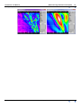
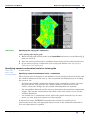
Below is an illustration of total horizontal derivative grids for continuation levels
112 m and 1655 m.
Library | Help | Top
© 2012 Intrepid Geophysics
| Back |
INTREPID User Manual
Library | Help | Top
Library | Help | Top
Multi-scale edge detection wizard (T44a)
22
| Back |
© 2012 Intrepid Geophysics
| Back |
INTREPID User Manual
Library | Help | Top
Interactive
Multi-scale edge detection wizard (T44a)
23
| Back |
Saving derivative grids—interactive
>> To specify the saving of horizontal derivative grids:
Library | Help | Top
1
Go to the Step 2—Pre-process and filter page.
2
Check the Save derivative grids checkbox.
3
Choose the corresponding Settings button. INTREPID displays the Save
derivatives—Settings dialog box.
4
Specify the precision for the saved grids, using the Grid Precision drop-down list.
See "Data Types in INTREPID datasets" in INTREPID database, file and data
structures (R05) for the available numeric data types.
5
Specify the prefixes for the derivative grids using the corresponding text boxes.
•
THD Prefix—Total horizontal derivative
•
XD Prefix—X derivative
•
YD Prefix—Y derivative
6
Specify the folder to contain the saved derivative grids, using the Grid Folder Path
text box.
7
Check the Save continuation grids checkbox. This is the original signal grid
upward continued at each level.
8
Also confirm the prefix and folder to save these grids
9
Choose Close.
© 2012 Intrepid Geophysics
| Back |
INTREPID User Manual
Library | Help | Top
Task files
Multi-scale edge detection wizard (T44a)
24
| Back |
Saving derivative grids—task files
1
PARMS job file syntax
Within the UC_Filtering Begin – End block:
•
Include the Output_Grids Begin – End block:
•
Use the Folder_Path keyword to specify the path of the folder for storing the
derivative grids, assigning a full or relative path.
•
Use the prefix keywords to specify the prefixes for the derivative grid filenames
(see Saving derivative grids—explanation for more about prefixes):
•
•
THD_Prefix—Total horizontal derivative
•
XD_Prefix—X derivative
•
YD_Prefix—Y derivative
Specify the precision of the saved derivative grids. Use the Grid_Precision
keyword, assigning the name of the data type. See "Data Types in INTREPID
datasets" in INTREPID database, file and data structures (R05) for a list.
Example:
Output_Grids Begin
Folder_Path = output/derivatives/
THD_Prefix = total_hz_deriv
XD_Prefix = x_deriv
YD_Prefix = y_deriv
Grid_Precision = IEEE4ByteReal
Output_Grids End
2
PROTOBUF task file syntax
message Output_Grids_INT {
optional string Folder_Path = 1 [default="output/grids"];
optional string THD_Prefix = 2 [default="total_hz_deriv"]; // the main grid used for edge
picking
optional string XD_Prefix = 3 [default="x_deriv"];
optional string YD_Prefix = 4 [default="y_deriv"];
optional ctm.GridDataTypes Grid_Precision = 5 [default=IEEE4ByteReal];
}
Library | Help | Top
© 2012 Intrepid Geophysics
| Back |
INTREPID User Manual
Library | Help | Top
Multi-scale edge detection wizard (T44a)
25
| Back |
Step 3—Calculate edge points
Parent topic:
Multi-scale edge
detection wizard
(T44a)
In this step you specify how INTREPID calculates the edge points that will make up
the worms. In this section:
•
Calculating edge points—options
•
Calculating edge points—interactive
•
Calculating edge points—task files
Below is an illustration of edge points derived from our case study grid.
Below is a 3D view of the points dataset. We exported the points dataset as VRML
(see Step 7—Export results) and viewed it using the Cosmo browser plug-in (see http:/
/www.karmanaut.com/cosmo/player/ or search for Cosmo player download) or the
Cortona VRML Client (see http://www.parallelgraphics.com/products/cortona/).
Library | Help | Top
© 2012 Intrepid Geophysics
| Back |
INTREPID User Manual
Library | Help | Top
Multi-scale edge detection wizard (T44a)
26
| Back |
Calculating edge points—options
Parent topic:
Step 3—
Calculate edge
points
You can specify the following options:
•
Whether to use the Euler method to estimate the depth of the calculated edge
points. If you do not require depth estimation, you can speed up processing
without it.
•
The method for calculating the edge points. Two methods are available—Canny
and Blakely & Simpson.
The Blakely & Simpson method involves sensing for a maximum across each of
several profiles within (usually) a 3 x 3 kernel. The number of profiles along which
maxima are found is used as a selection criteria. Too many maxima points are
generated if acceptance is based on only one profile requiring a maximum, and
best results are obtained when at least three are required. The position of a
selected maximum within each kernel computation is not restricted to a grid cell
point. INTREPID fits a cubic function to the three points and the maximum of
this function obtained.
The Blakely & Simpson method requires a parameter—the minimum size of an
anomaly for INTREPID to include a point. This is the minimum difference
required of the cell from the average of the surrounding cells. If the difference is
larger, INTREPID identifies an edge point at the position of the cell. This
parameter is in the units of the signal in the cell per distance unit, generally
mGal/m or nT/m. If you give the parameter the value 0, then INTREPID selects
all anomalies.
The Canny method also uses a 3 x 3 kernel, but in this case one profile is used for
sensing a maximum, and its direction is that of the main field gradient.
INTREPID needs to calculate this direction before applying the method. The
computed maxima are not restricted to a grid cell location. INTREPID
interpolates them using a cubic function.
The results of the Canny method are generally better by a small margin. Both
methods give good results when the signal to noise ratio is large, but extraction of
reliable points is not easy in noisy data.
Both these methods have also been adapted for use with tensor gradient grids.
Other edge picking algorithms are also in trial. A recussive Gaussian filter, as
used in medical imaging, may be available soon.
•
Library | Help | Top
Whether to save the output edge points dataset, and the path and file name for it.
See Structure of output edge point datasets for dataset details.
© 2012 Intrepid Geophysics
| Back |
INTREPID User Manual
Library | Help | Top
Multi-scale edge detection wizard (T44a)
27
| Back |
Calculating edge points—interactive
Parent topic:
Step 3—
Calculate edge
points
See Calculating edge points—options for information about the options.
Interactive
1
Go to the Step 3—Calculate edge points page.
2
(If you want INTREPID to estimate depths of the calculated edge points) Check the
Estimate depth of points using the Euler method checkbox.
3
Select the edge Points calculation method from the drop-down list.
4
Specify the Minimum anomaly size for including point in the corresponding text
box. This is essentially a noise rejection option. It is set to a low value - 0.00005 as
a starting value, and is progressively made smaller as the upwards continuation
process proceeds. If you feel you are not getting enough WORMS, turn off this
option by setting the value to 0.0.
5
(If you want to save the calculated edge points dataset):
Library | Help | Top
>> To specify edge point calculation:
•
Check the Save output edge points dataset checkbox.
•
Specify the path and name for the dataset in the Edge points dataset text box
or use the browse [...] button to specify it.
© 2012 Intrepid Geophysics
| Back |
INTREPID User Manual
Library | Help | Top
Multi-scale edge detection wizard (T44a)
28
| Back |
Calculating edge points—task files
Parent topic:
Step 3—
Calculate edge
points
Task files
See Calculating edge points—options for information about the options.
1
PARMS job file syntax
Within the Vector_Processing Begin – End block:
•
Include the Point_Picking Begin – End block:
•
Use the Point_Depth_Estimation keyword to specify whether you want
INTREPID to estimate depths of the calculated edge points—assign yes or no.
•
Use the Name keyword to specify the edge points calculation method—assign
Blakely or Canny.
•
(If you selected the Blakely method) Use the Minimum_Anomaly keyword to
specify the minimum size of an anomaly for INTREPID to calculate an edge
point—assign a numeric value.
•
Specify the path and filename of the calculated edge points dataset. Use the
Point_Dataset keyword, assigning the path and file name for the dataset. Omit
the line if you do not want to save the dataset.
Example:
Point_Picking Begin
Point_Dataset= output/points..DIR
Point_Depth_Estimation= no
Name = Blakely
Minimum_Anomaly= 0.000000
Point_Picking End
2
PROTOBUF task file syntax
point {
Minimum_Anomaly: 0.0000; # way to reject more subtle surface features, this
is also scaled as we go upwards
Point_Dataset: "../datasets/output/points..DIR";
Method: Canny;
Amplitiude_Option: TotalHorizontal;
}
Library | Help | Top
© 2012 Intrepid Geophysics
| Back |
INTREPID User Manual
Library | Help | Top
Multi-scale edge detection wizard (T44a)
29
| Back |
Step 4—Group edge points into 'worms'
Parent topic:
Multi-scale edge
detection wizard
(T44a)
In this step you specify how INTREPID groups the edge points to form worms and
saves this data in a line dataset. In this section:
•
Group edge points into worms—options
•
Group edge points into worms—interactive
•
Group edge points into worms—task files
Below is an illustration of worms derived from the edge points of our case study grid.
Group edge points into worms—options
Parent topic:
Step 4—Group
edge points into
'worms'
Library | Help | Top
You can specify the following options:
•
The maximum distance allowed between edge points that INTREPID groups into
a worm. We recommend 2 cell widths.
•
Whether to save the worms dataset, and the path and file name for it. See
Structure of output worm line datasets for dataset details.
•
At this stage, you also get to request a true depth to the worm, at ecah
continuation level. In the early tests for this method, it was noticed that
approximately 0.5 times the continuation height, was a reasonable first estimate
of the worm depth. This remains a default estimate of the depth. A more serious
attempt can be made by calling on the Euler Deconvolution mdifferential
equations, especially adapted and modified for this context. In particular, nmore
enmphasis is placed on the vertical components, as the X & Y location of the
source is assumed to be the calculated “worm” position. We add the 2 Hilbert
transforms to the vertical component, and use 2 observation points or pairs of
points down thje worm, to directly solve for the depth and the structural index.
Any inadmissable values are rejected, and we simplify the depth and SI estimate
to an average value for each worm at each continuation level.
•
The stratgety for an FTG signal is different to this, as we have measured
gradients for all components.
© 2012 Intrepid Geophysics
| Back |
INTREPID User Manual
Library | Help | Top
Multi-scale edge detection wizard (T44a)
30
| Back |
Group edge points into worms—interactive
Parent topic:
Step 4—Group
edge points into
'worms'
See Group edge points into worms—options for information about the options.
Interactive
1
Go to the Step 4—Group edge points into worms page.
2
Specify the Maximum distance between edge points (in cell widths) in the
corresponding text box.
3
You can save a GeoTiff of the amplitude of each picked point at each level, burnt
into an image file. This is very convienent for rapid interpretation within a GIS
package, or even within Geomodeller, when you wish to reconcile the 3D fault/
contact surfaces with the original picks.
4
A temporary standard geophysical grid “ wormsTemp.ers” is used as an
intermeditary place to accumulate the results needed for this image.
5
(If you want to save the worms line dataset):
>> To specify edge point grouping into worms:
•
Check the Save output worms line dataset checkbox.
•
Specify the path and name for the dataset in the Worms dataset text box or
use the browse [...] button to specify it. By default this is an Intrepid format
line database.
Group edge points into worms—task files
Parent topic:
Step 4—Group
edge points into
'worms'
Task files
See Group edge points into worms—options for information about the options.
1
PARMS job file syntax
Within the Vector_Processing Begin – End block:
•
Include the Worm_Processing Begin – End block:
•
Use the Maximum_Point_Separation keyword to specify maximum distance
allowed (in cell widths) between edge points that INTREPID groups into a
worm—assign a numeric value.
•
Specify the path and filename of the worms dataset. Use the Worm_Dataset
keyword, assigning the path and file name for the dataset. Omit the line if you do
not want to save the dataset.
Example:
Worm_Processing Begin
Maximum_Point_Separation= 2.0
Library | Help | Top
© 2012 Intrepid Geophysics
| Back |
INTREPID User Manual
Library | Help | Top
Multi-scale edge detection wizard (T44a)
31
| Back |
Worm_Dataset= output/worms..DIR
Worm_Processing End
2
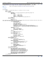
PROTOBUF task file syntax
worm {
Maximum_Point_Separation: 2.0; # units of cell size
Worm_Dataset: "../datasets/output/worms..DIR";
Worm_Min_Nr_Points: 3; # minimum required length of a worm in points
Worm_Image: "wormImage.tif";
Euler_Minimum_Gradient_Amplitude: 0.3; # nT/m
Depth_Estimation: true; # also estimate a local best Euler decon depth
estimate
}
In this case, you can see previously undocumented features. This is one of the big
benefits of a published data model for each of the tools, especially if the file published
tells the truth. In this case, the intrepid-tasks.proto published file, is exactly the same
one used to build the whole software base, so it is guarenteed to tell the truth.
So, extra stuff here -
Library | Help | Top
•
a tif file with the worms burnt in as a image
•
New signal/noise parameter to stop generating points when the amplitude of the
signal is below a noise floor.
•
Flag to ask for Euler deconvolution work
© 2012 Intrepid Geophysics
| Back |
INTREPID User Manual
Library | Help | Top
Multi-scale edge detection wizard (T44a)
32
| Back |
Step 5 - Calculate linears
Parent topic:
Multi-scale edge
detection wizard
(T44a)
In this step you specify how INTREPID produces a straight line segment (linear) that
simplifies the edges of the inferred structure. In this section:
•
Calculate linears—options
•
Calculate linears—interactive
•
Calculate linears—task files
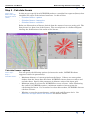
Below are illustrations of linears derived from the worms of our case study grid. The
first picture is a plan view of the linears. The second picture is a balloon diagram
showing the distribution of the strike of the linears.
Calculate linears—options
Parent topic:
Step 5 Calculate linears
Library | Help | Top
You can specify the following options (in interactive mode, INTREPID shows
suggested values for parameters):
•
Maximum distance of a worm point from the linear. If there are worm points
further from the linear than this limit, INTREPID classes them as outliers and
excludes them. Specify this parameter in distance units of the input grid.
•
Minimum points in a worm for INTREPID to create a linear. After eliminating
the outliers, INTREPID requires a minimum number of worm points for
calculating the linear. If a worm has less than this number, INTREPID does not
calculate a linear.
•
Whether to save the worms dataset, and the path and file name for it. See
Structure of output linears line datasets for dataset details.
© 2012 Intrepid Geophysics
| Back |
INTREPID User Manual
Library | Help | Top
Multi-scale edge detection wizard (T44a)
33
| Back |
Calculate linears—interactive
Parent topic:
Step 5 Calculate linears
See Calculate linears—options for information about the options.
Interactive
1
Go to the Step 5—Calculate linears page.
2
Specify the Maximum deviation of worm points from a linear in the
corresponding text box.
3
Specify the Minimum number of points in a linear in the corresponding text box.
4
(If you want to save the linears line dataset):
>> To specify calculating linears:
•
Check the Save linear dataset checkbox.
•
Specify the path and name for the dataset in the Linear dataset text box or use
the browse [...] button to specify it.
Calculate linears—task files
Parent topic:
Step 5 Calculate linears
Task files
See Calculate linears—options for information about the options.
Within the Vector_Processing Begin – End block:
•
Include the Line_Processing Begin – End block:
•
Use the Maximum_Straight_Line_Deviation keyword to specify maximum
distance from a worm point to a linear—assign a numeric value in input dataset
distance units.
•
Use the Minimum_Points_For_Linear keyword to specify the minimum
number of points required in a worm for INTREPID to create a linear—assign a
numeric value.
•
Specify the path and filename of the linears dataset. Use the Linear_Dataset
keyword, assigning the path and file name for the dataset. Omit the line if you do
not want to save the dataset.
Example:
Line_Processing Begin
Maximum_Straight_Line_Deviation= 8000.0
Minimum_Points_For_Linear= 15
Linear_Dataset= output/linears..DIR
Line_Processing End
Library | Help | Top
© 2012 Intrepid Geophysics
| Back |
INTREPID User Manual
Library | Help | Top
Multi-scale edge detection wizard (T44a)
34
| Back |
Step 6 - Calculate 3D Surfaces
You can create 3D surfaces from the worms that you have already calculated. This is
done semi-automatically at present. The clustering algorithm works by starting at
the greatest level, taking worms that exist, and then searching all the other levels for
near fits in an XY spatial sense, near striuke sense, and minimum length. Total
horizontal gradient, and total curvature gradient can also be used for picking, when
an FTG signal source is being used. Typically, a smaller number of 3D surfaces is
created this way, than the total number of worms at the greatest continuatiopn level,
due to the extra constraints being placed upon the surface. As the intent is to
automatically create something like a fault network in 3D, in a short timeframe,
efforts are made to also estimate dip and limited fault extents. Every effort is made to
make 3 ASCII csv files that are compatible with the 3D import options inside
Geomodeller, resulting in contacts that form 3D surfaces caulated from the interface
points, foliations and the limits.
Calculate surfaces—options
Parent topic:
Step 5 Calculate linears
You can specify the following options (in interactive mode, INTREPID shows
suggested values for parameters):
•
Maximum distance of a worm point from the linear at each 3D continuation level.
If there are worm points further from the linear than this limit, INTREPID
classes them as outliers and excludes them. Specify this parameter in distance
units of the input grid.
•
Minimum points in a worm for INTREPID to create a surface. After eliminating
the outliers, INTREPID requires a minimum number of worm points for
calculating the surface. If a worm has less than this number, INTREPID does not
calculate a surface using this worm.
•
Minimum number of co-located worms in a 3D stack, to then move to a coherent
surface - defalut is 3.
•
When clustering worms at differering levels, the polylines might cross rather than
be semi-parallel. To check for this and reject a join, a maximum strike angle
divergence can be specified - default is 45.
•
The option of subsampling the interface points at each level - the default is to take
start and end points and every 5th point.
•
Whether to save the surface dataset, and the path and file name for it.
•
1
PROTOBUF task file syntax
surfaces { # here is the extension to 3D contacts, export to Geomodeller, does feature clustering and
estimate a dip/strike
Maximum_Straight_Line_Deviation: 8000.0;
Minimum_Points_For_3D: 15;
Contact_Dataset: "../datasets/output/contacts3d"; # stub for the 3 output csv files
drape { # flying elevation grid of survey
type: Elevation;
mean_elevation: 200;
# grid: ; # named grid
}
style: ALL; # go for all the indicated contacts, not just the linears
Strike_Divergence: 45 # when joining worms that cross at different levels
DoSubSample: true # only save every 5th point plus beginning and end for each level
}
An important new aspect that emerges here, is the requirement to get the elevations
Library | Help | Top
© 2012 Intrepid Geophysics
| Back |
INTREPID User Manual
Library | Help | Top
Multi-scale edge detection wizard (T44a)
35
| Back |
properly tied to the DTM. For that purpose, either a notional mean_elevation for a
survey is required, or, better, supply a proper DTM grid, so that each worm has
corrected below surface attributed depths.
As with the linears, the 3D worms can also be restrited to mostly linear features. The
new clustering algorithm starts at the deepest level, and then chases back up through
the preceeding levels, looking for best fit joins in a vertical sense.
Look at the report file, to get a sense of the number of segments involved, and the
success or otherwise of this process.
Written 28 fault features from possible 52 to file output/contacts_interface_contacts.csv
Written 28 fault orientations from possible 52 to file output/contacts_orientation_contacts.csv
Written 28 limited fault extents from possible 52 to file output/contacts_limited_extents.csv
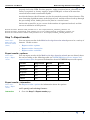
Step 7—Export results
Parent topic:
Multi-scale edge
detection wizard
(T44a)
You can export results of the Multi-scale edge detection wizard process in a variety of
formats. In this section:
•
Export results—options
•
Export results—interactive
•
Export results—task files
Export results—options
Parent topic:
Step 7—Export
results
You can export results of the Multi-scale edge detection wizard process directly from
the tool according to the following table (see INTREPID direct access, import and
export formats (R11) for general information about INTREPID import and export):
Format
Edge Points
Worms
Linears
ASCII
Yes
Yes
Yes
ArcShape
Yes
Yes
MapInfo
Yes
Yes
gOcad
Yes
Yes
VRML
Yes
Export results—interactive
Parent topic:
Step 7—Export
results
See Export results—options for information about the options.
Interactive
1
Library | Help | Top
>> To specify calculating linears:
Go to the Step 7—Export results page.
© 2012 Intrepid Geophysics
| Back |
INTREPID User Manual
Library | Help | Top
2
Library | Help | Top
Multi-scale edge detection wizard (T44a)
36
| Back |
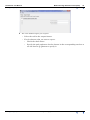
For each dataset export you require:
•
Select the tab for the output format.
•
For the datasets that you want to export:
•
Check the check boxes.
•
Specify the path and name for the dataset in the corresponding text box or
use the browse [...] button to specify it.
© 2012 Intrepid Geophysics
| Back |
INTREPID User Manual
Library | Help | Top
Multi-scale edge detection wizard (T44a)
37
| Back |
Export results—task files
Parent topic:
Step 7—Export
results
See Export results—options for information about the options.
•
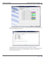
Include the Supplementary_Outputs Begin – End block:
Task files
•
Use the keywords shown in the table below to specify the paths and filenames of
the exported datasets that you require:.
Format
Dataset
Keyword
ASCII
Edge Points
Ascii_Point_Dataset
Worms
Ascii_Worm_Dataset
Linears
Ascii_Line_Dataset
Edge Points
ArcShape_Point_Dataset
Worms
ArcShape_Worm_Dataset
Edge Points
MapInfo_Point_Dataset
Worms
MapInfo_Worm_Dataset
Edge Points
GoCad_Point_Dataset
Worms
GoCad_Worm_Dataset
Edge Points
Vrml_Point_Dataset
ArcShape
MapInfo
gOcad
VRML
Example
Supplementary_Outputs Begin
Ascii_Point_Dataset= output/asciiPts.wrm
Ascii_Worm_Dataset= output/asciiWorms.str
Ascii_Line_Dataset= output/asciiLines.lin
ArcShape_Point_Dataset= output/arcshapePts.shp
ArcShape_Worm_Dataset= output/arcshapeWorms.shp
MapInfo_Point_Dataset= output/mapInfoPts.mif
MapInfo_Worm_Dataset= output/mapInfoWorms.mif
GoCad_Point_Dataset= output/gocadPts.cad
GoCad_Worm_Dataset= output/gocadWorms.pl
Vrml_Point_Dataset= output/vrmlPts.wrl
Supplementary_Outputs End
Library | Help | Top
© 2012 Intrepid Geophysics
| Back |
INTREPID User Manual
Library | Help | Top
Multi-scale edge detection wizard (T44a)
38
| Back |
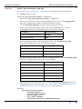
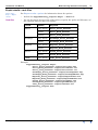
Example GeoTIFF image
If required, the WormE tool produces a geoTiff image of the points
picked at each continuation level, stacked by adding the Total
Horizontal derivative anomaly magnitude at each cell centroid.
Library | Help | Top
© 2012 Intrepid Geophysics
| Back |
INTREPID User Manual
Library | Help | Top
Multi-scale edge detection wizard (T44a)
39
| Back |
Specifying input and output files
Parent topic:
Multi-scale edge
detection wizard
(T44a)
INTREPID has controls for specifying the input and output datasets at logical places
in the wizard and some controls in the File menu.
You can enter the path and ..DIR or .ers file name of the datasets in the dataset
text boxes or browse using the [...] buttons. If you browse, INTREPID displays an
Open or Save As dialog box. Use the directory and file selector to locate the file you
require. (See "Specifying input and output files" in Introduction to INTREPID (R02)
for information about specifying files).
INTREPID may need to obtain information from the dataset aliases. In the output
vector datasets it creates the following aliases.
Alias
Field
X
X coordinate (geographic location)
Y
Y coordinate (geographic location)
See "Vector dataset field aliases" in INTREPID database, file and data structures
(R05) for more information about aliases.
In this section:
•
File menu options
•
Input and output datasets in wizard pages
•
Structure of output edge point datasets
•
Structure of output worm line datasets
•
Structure of output linears line datasets
File menu options
Parent topic:
Specifying input
and output files
Load Options If you want to use an existing task specification file to specify the
Multi-scale edge detection wizard process, use this option to specify it.
INTREPID loads the file and uses its contents to set all of the parameters for the
Multi-scale edge detection wizard process. (See Creating and using task
specification files for more information).
Save Options If you want to save the current Multi-scale edge detection wizard file
specifications and parameter settings as a task specification file, use this option to
specify the filename and save the file. (See Creating and using task specification
files for more information).
Open Input Dataset Use this command to specify the input grid dataset. This is the
same as using the browse [...] button in the Input Grid page. See Step 1—Specify
input dataset, scalar TMI grid example for more information.
Library | Help | Top
© 2012 Intrepid Geophysics
| Back |
INTREPID User Manual
Library | Help | Top
Multi-scale edge detection wizard (T44a)
40
| Back |
Input and output datasets in wizard pages
Parent topic:
Specifying input
and output files
The instructions for specifying input and output datasets are in appropriate places in
the wizard pages:
•
Input datasets:
•
•
Input grid dataset—see Step 1—Specify input dataset, scalar TMI grid
example.
Output datasets (all optional, depending on your requirements):
•
Subsection of the input grid dataset—see Step 1—Specify input dataset, scalar
TMI grid example
•
Intermediate FFT datasets: Expanded, Windowed, FFT—see Step 2—Preprocess and filter and Saving FFT products
•
Intermediate filter results: Horizontal derivative—see Step 2—Pre-process
and filterand Saving derivative grids
•
Point dataset with edge points (in INTREPID native or other format)—see
Step 3—Calculate edge points and Step 7—Export results
•
Line dataset with worms (in INTREPID native or other format)—see Step 4—
Group edge points into 'worms' and Step 7—Export results
•
Line dataset with linears (regressed line segments) (in INTREPID native or
other format)—see Step 5 - Calculate linears and Step 7—Export results
•
3D surface interface, orientation and fault extents in comma seperated file
format.
•
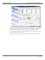
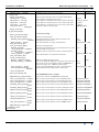
A process report file that summarises the options used for each run of the tool,
adn records what was found and where things got stored. For example -
Summary of continuation
Level
Library | Help | Top
Height
CellSize Points
Segments Linears found
0
112.00
80.0000
3105
200
61
1
157.00
80.0000
2618
150
49
2
220.00
80.0000
2112
119
50
3
308.00
80.0000
1730
90
34
4
431.00
80.0000
1326
56
29
5
603.00
80.0000
986
36
19
6
844.00
80.0000
704
28
15
7
1182.00
80.0000
577
13
10
8
1655.00
80.0000
550
12
8
© 2012 Intrepid Geophysics
| Back |
INTREPID User Manual
Library | Help | Top
Multi-scale edge detection wizard (T44a)
41
| Back |
Structure of output edge point datasets
Parent topic:
Specifying input
and output files
Library | Help | Top
The output edge point dataset contains the edge points calculated in Step 3 of the
worming process.
Output edge point datasets have the following fields
Field
Description
X
East–West geographic location
Y
North–South geographic location
amplitude
Magnitude of signal at the point
Cont_Ht
Continuation level at which INTREPID inferred the edge
point (‘group by’ field)
Strike
Estimate of direction of any detected edge (based on values
in the 9 grid cells (3 x 3 matrix) that include the point)
CellSize
Cell size of grid ('group by' field)
Window
Size of Euler window.
© 2012 Intrepid Geophysics
| Back |
INTREPID User Manual
Library | Help | Top
Multi-scale edge detection wizard (T44a)
42
| Back |
Structure of output worm line datasets
Parent topic:
Specifying input
and output files
INTREPID associates nearby edge points to infer edges and produce ‘worms’. In the
output worm line dataset, each line is an inferred edge.
Output worm line datasets have the fields shown in the following table. The worms
are grouped by continuation height.
Depth and SI fields should only appear in the worm line dataset if Euler point depth
estimation is used.
Library | Help | Top
Field
Description
X
East–West geographic location
Y
North–South geographic location
Depth
Depth estimate for the edge point - optional.
SI
Structural index of inferred structure - optional (see
"Structural Index" in Euler Deconvolution (T44))
Cont_Ht
Continuation level at which INTREPID inferred the edge
point (‘group by’ field)
amplitude
Magnitude of signal for the edge point
© 2012 Intrepid Geophysics
| Back |
INTREPID User Manual
Library | Help | Top
Multi-scale edge detection wizard (T44a)
43
| Back |
Structure of output linears line datasets
Parent topic:
Specifying input
and output files
INTREPID performs linear regression on each ‘worm’ to produce a straight line
segment (linear) that simplifies edges in the inferred structure. In the output linears
line dataset, each line shows the strike and length of an inferred edge.
Output linears line datasets have the fields shown in the following table. The linears
are grouped by continuation height.
Depth and SI fields should only appear in the linears line dataset if Euler point depth
estimation is used..
Library | Help | Top
Field
Description
X
East–West geographic location of the end point
Y
North–South geographic location of the end point
amplitude
Magnitude of signal at the end point
Depth
Depth estimate for the end point - optional
Cont_Ht
Continuation level at which INTREPID inferred the
corresponding edge points and worm (‘group by’ field—
same value for both points)
SI
Structural index of inferred structure - optional (see
"Structural Index" in Euler Deconvolution (T44)) (‘group
by’ field—same value for both points)
Linearity
Measure of linearity of the worm using least squares fit—
small values indicate relatively straight worm (‘group by’
field—same value for both points)
Strike
Direction of the linear (‘group by’ field—same value for
both points)
Points
Number of points in the worm used for the linear (‘group
by’ field—same value for both points)
© 2012 Intrepid Geophysics
| Back |
INTREPID User Manual
Library | Help | Top
Multi-scale edge detection wizard (T44a)
44
| Back |
Structure of Worm3D surface datasets
Parent topic:
Specifying input
and output files
INTREPID performs cluster analysis on each ‘worm’ at the highest continuation level
to produce a family of related interface points, foliations and limited fault extents
estimated from each cluster. In the output 3D surface dataset, part A is for interface
points, part B is for foliations and part C is for fault limited radii.
•
A - Output interface points have the fields “ContactNumber, X,Y,Depth,Anomaly”
shown in the following example.
// Intrepid WormE 3D contacts, Projection: TMAMG54, Datum: AGD66
// Intrepid assumes the solutions are below a aero-survey drape surface (zero value),
with Z positive upwards
Contact,Easting,Northing,Elevation,Anomaly
Contact1,747276.187500,8416132.000000,-215.500000,3.284356
Contact1,747582.562500,8415519.000000,-215.500000,4.026762
Contact1,747705.250000,8414906.000000,-215.500000,3.754344
•
B - Output foliation points have the fields “ContactNumber,
X,Y,Depth,DipDirection,Dip” shown in the following example.
// Intrepid WormE 3D contact orientations, Projection: TMAMG54, Datum: AGD66
// Intrepid assumes the solutions are below a aero-survey drape surface (zero value),
with Z positive upwards
// This file also must be imported by Geomodeller along with the contacts, to define
enough constraints to create fault surfaces
Contact,Easting,Northing,Elevation,DipDirection,Dip,Polarity
Contact1,747693.8,8415176.1,-215.5, 246.0, 36.5, 1
Contact1,747086.2,8416655.0,-422.0, 253.0, 61.2, 1
Contact2,750123.0,8419553.1,-110.0, 229.0, 64.1, 1
•
C - Output limited fault radii so that each 3D worm can be treated as having
limited extent when rendered within Geomodeller, and allowing the user to
merge, delete, and decide on the fault network order
// Intrepid WormE 3D contact limited extents box, Projection: TMAMG54, Datum: AGD66
// Intrepid assumes the solutions are below a aero-survey drape surface (zero value),
with Z positive upwards
// This file also must be imported by Geomodeller along with the contacts, to define
enough constraints to create a limited fault surface
Contact,HorizontalRadius,VerticalRadius,InfluenceDistance
Contact1,5047.2,3310.0,1394.6
Contact2,4177.6,3310.0,1245.1
Contact3,8534.5,3310.0,997.3
Contact4,8801.9,3310.0,3025.5
Geomodeller Project Import and fault network Creation
The process of bringing the womrs3D interface/foliation data into Geomodeller and
creating a Fault network is described. You need to also have a copy of the
Geomodeller tool available and open, ready to use. A very small example project is
distributed within the examples/geomodeller_projects/mlevel_example/
Library | Help | Top
© 2012 Intrepid Geophysics
| Back |
INTREPID User Manual
Library | Help | Top
Multi-scale edge detection wizard (T44a)
45
| Back |
worme_example data area. The project is an xml file called “wormeexample.xml”
Open this project within geomodeller and you should arrive at the following
unpopulated 3D geology model .
From there, choose import>3DGeology> interfaces
You then go through a series of wizard screen, to bring these 3D points into your
project.
Library | Help | Top
© 2012 Intrepid Geophysics
| Back |
INTREPID User Manual
Library | Help | Top
Multi-scale edge detection wizard (T44a)
46
| Back |
Now press NEXT and then toggle the top 3 comment lines, so that the first line in the
import screen is the first interface datapoint.
Press NEXT and then review the requirement for the 3D interfrace import option to
have a geology Formation, X,Y and Z field.
Library | Help | Top
© 2012 Intrepid Geophysics
| Back |
INTREPID User Manual
Library | Help | Top
Multi-scale edge detection wizard (T44a)
47
| Back |
Press NEXT and then toggle the ALL drop down list to choose “CREATE FAULT”.
With this option chosen, the import wizard will also crete Faults in the project, give
them a disticnt colour code, and then associate each set of 3D points with the correct
fault unit.
Press FINISH to complete the interface import.
The import report will look like the following.
Library | Help | Top
© 2012 Intrepid Geophysics
| Back |
INTREPID User Manual
Library | Help | Top
Multi-scale edge detection wizard (T44a)
48
| Back |
Repeat the same process now for the other two exported Worm3D files.
Firstly, the orientation dataset - choose Import>3DGeology>Orientation Data.
After NEXT, you will see the importer wanting to join the orientation 3D data with
the previous interface data. This is shown by the wizard panel’s default action
“Import” offering to Merge with the known Fault/Contacts.
Library | Help | Top
© 2012 Intrepid Geophysics
| Back |
INTREPID User Manual
Library | Help | Top
Multi-scale edge detection wizard (T44a)
49
| Back |
After selecting FINISH, you are given a report that tells you how many foliation data
points were added to your project.
To finish the process, repeat much the same steps, this time choosing
Import>3DGeology>Fault Limits. The following screen shows a point partly through
the wizard process, where you are setting the influence radius of each of the 3
directions for the fault axes.
Library | Help | Top
© 2012 Intrepid Geophysics
| Back |
INTREPID User Manual
Library | Help | Top
Multi-scale edge detection wizard (T44a)
50
| Back |
Now we have a set of viable conditions to create a 3D fault surfaces, directly from the
wormE tool, with an ability to verify the spatial 2D relationships, as traditionally
done using a GIS, with the full power of a 3D fault network interpretation.
So, in a short form explanation, compute the geology model Model>Compute, then
choose Faults Only. select all contacts.
Display the topographic expression of the faults. Model > Plot the model settings
Library | Help | Top
© 2012 Intrepid Geophysics
| Back |
INTREPID User Manual
Library | Help | Top
Multi-scale edge detection wizard (T44a)
51
| Back |
Then in 3D, build 3D shapes, and show fault surfaces.
The quality of the initial fault network is quite dependent on the survey data. Good
quality gravity and FTG data will give a very credible automatic model, which can
rapidly be improved using the Merge faults tool.
Library | Help | Top
© 2012 Intrepid Geophysics
| Back |
INTREPID User Manual
Library | Help | Top
Multi-scale edge detection wizard (T44a)
52
| Back |
Dealing with FTG survey data
With V4.5, this tool has also been adapted to have a workflow that accomodates full
tensor gradient data, provided it is presented as a regular grid, with each cell of the
grid having a best estimate of the field curvature gradients. This is accomplised easily
enough using the Intrepid gridding tool. As with the scalar data case already
described, the best result can be obtained by doing as little filtering to the original
survey data as possible, so best results come from using tensors that have been
measured. The full tensor gravity, magnetics survey data is well suited for this task.
As it happens, Falcon is also a reasonable candidate, as the measured gradient pair,
often called the horizontal curvate gradient, is similar to conventional measures.
The Falcon tensor workflow remain to finalized, as the initial emphasis has been on
FTG. The maximum horizontal curvature anomaly ( Txy,Tuv) of the Falcon,
represents a depature from a perfect spherical body, as opposed to the maximum
horizontal gradien ( Tzx,Tyz), as used traditionally. This later quantity represents
contact edges.
All upwards continuation work is done on the tensor grid signal. This option can also
be found in the gfilt tool.
Step 1—Specify input dataset, Tensor Gravity Gradient grid example
Parent topic:
Multi-scale edge
detection wizard
(T44a)
In this step you can specify:
•
Input grid and band—see Specifying the input grid
•
Subsection of input grid—see Specifying a subsection of the input grid
Specifying the input grid
Parent topic:
Step 1—Specify
input dataset,
scalar TMI grid
example
In this section:
•
Specifying the input grid—interactive
•
Specifying the input grid—batch files
Note: The current version of this tool only supports projected input grids with metres
as distance unit.
Below is an illustration of a grid that we shall use as a case study in this chapter. It is
the Brazilian dataset called Aurizonia and can be found in the cookbook>tensor
section.
This data was acquired around 2007 and the geology context is one of rolling sand
dunes in a swampy environment with suspected gas accumaltions that are not that
deep. The data was provided by the exploration company, via Bell Geoscience. There
is also the SRTM digital terrain data provided in the same cookbook area.
Library | Help | Top
© 2012 Intrepid Geophysics
| Back |
INTREPID User Manual
Library | Help | Top
Interactive
Multi-scale edge detection wizard (T44a)
53
| Back |
Specifying the input grid—interactive
>> To specify the input grid:
1
Enter the full path and file name in the Input Grid text box or use the Browse [...]
button to locate it.
2
Note, the tensor grid reference coordiante frame is noted next to the band chooser.
3
(If you want to specify a subsection of the input grid dataset) See Specifying a
subsection of the input grid.
Specifying upward continuation levels for tensor grids
Parent topic:
Step 2—Preprocess and filter
In this section:
Specifying upward continuation levels—explanation
The selection of levels depends on the number of levels required, the grid cell size and
the smallest dimension of the survey. We recommend the following way of deciding
the levels to use:
•
Calculate the upward continuation heights using a multiplier of about 1.6 times
the grid cell size. This provides for a greater density of levels nearer to the
surface, where the changes are more rapid, thinning them out upwards.
•
Use the smallest dimension of the survey to determine the maximum continuation
height. The upward continuations have little value after about 0.1 to 0.2 of the
smallest dimension.
•
use around 6 or 7 continuation levels, and as the signal attenuates by on extra
power ( eg cube instead of square for scalar signals).
In interactive mode, INTREPID automatically calculates a suitable set of
continuation levels for your input grid dataset based on the method described here.
You can adjust them as required
Library | Help | Top
© 2012 Intrepid Geophysics
| Back |
INTREPID User Manual
Library | Help | Top
Interactive
Multi-scale edge detection wizard (T44a)
54
| Back |
Specifying upward continuation levels—interactive
>> To specify upward continuation levels:
Library | Help | Top
1
Go to the Step 2—Pre-process and filter page
2
The adaptation for tensors has simplified this panel, and the 2 horizontal gradient
options are available. However, just use the total horizontal gradient for now.
3
The save grids option allows you to see the daughter products use in the actual
picking and depth estimation work.
© 2012 Intrepid Geophysics
| Back |
INTREPID User Manual
Library | Help | Top
Multi-scale edge detection wizard (T44a)
55
| Back |
All further options are common to the previous tutorial descriptions. The next image
shows the stacked “worms” for this dataset in the Intrepid Visual tool. The amplitude
field is used to colour code the polylines. The deeper, more important contacts, are
shown in red.
Summary of continuation
Level
Library | Help | Top
Height
CellSize Points
Segments Linears found
0
80.00
50.0000
9827
945
99
1
244.00
50.0000
5326
373
113
© 2012 Intrepid Geophysics
| Back |
INTREPID User Manual
Library | Help | Top
Multi-scale edge detection wizard (T44a)
56
| Back |
2
990.00
50.0000
1816
63
30
Help
Parent topic:
Multi-scale edge
detection wizard
(T44a)
When you point to an element in the Multi-scale edge detection wizard, it displays
help information about the element.
You can use the Help menu to display further information about this tool.
Apply
Parent topic:
Multi-scale edge
detection wizard
(T44a)
When you choose Finish on Step 7—Export results INTREPID executes the Multiscale edge detection wizard task.
Exit
Parent topic:
Multi-scale edge
detection wizard
(T44a)
Library | Help | Top
To exit from Multi-scale edge detection wizard choose Exit from the File menu or the
Cancel button.
© 2012 Intrepid Geophysics
| Back |
INTREPID User Manual
Library | Help | Top
Multi-scale edge detection wizard (T44a)
57
| Back |
Task specification (.job) files
Parent topic:
Multi-scale edge
detection wizard
(T44a)
This section gives an overview, example and describes the syntax of Multi-scale edge
detection wizard task specification files.
In this section:
•
Finding out more about task files and batch processing mode
•
Main block structure of an Multi-scale edge detection wizard task file
•
Sample Multi-scale edge detection wizard task specification (.job) file
•
Syntax table
•
Creating and using task specification files
Finding out more about task files and batch processing mode
Parent topic:
Task
specification
(.job) files
Use the following references:
Introduction to INTREPID auxiliary files,
such as task files
"INTREPID Auxiliary files" in INTREPID database,
file and data structures (R05)
Structure, syntax and use of INTREPID task
files
INTREPID task specification (.job) files (R06)
Running INTREPID in batch processing
mode
"How to start INTREPID—Overview" in Introduction
to INTREPID (R02)
Main block structure of an Multi-scale edge detection wizard task file
Parent topic:
Task
specification
(.job) files
The following table shows the main block structure of a Multi-scale edge detection
wizard task file. See Syntax table for more details.
Block definition
Contents
Process Begin
Task file outer block
—Tool name and date stamp
—Parameters block
——Input grid block
———Grid filename and band
...
Parameters Begin
Input_Grid Begin
...
Input_Grid End
UC_Filtering Begin
...
——Upward continuation grid filtering block
———FFT, IGRF and filter parameters
UC_Filtering End
Vector_Processing Begin
...
——Vector processing block
———Output vector datasets and parameters
Vector_Processing End
Supplementary_Outputs Begin
...
——Supplementary outputs block
———Outputs in non-INTREPID-native formats
Supplementary_Outputs End
Parameters End
Process End
Library | Help | Top
—End
End
© 2012 Intrepid Geophysics
| Back |
INTREPID User Manual
Library | Help | Top
Multi-scale edge detection wizard (T44a)
58
| Back |
Sample Multi-scale edge detection wizard task specification (.job) file
Parent topic:
Task
specification
(.job) files
Here is an example of an Multi-scale edge detection wizard task.
Process Begin
Comments= "Intrepid Audit Stamp v3.7 (release) cut 267-11/ 5/2004"
Name
= WormE
Parameters Begin
Input_Grid Begin
Input_Grid= C:\Intrepid\cookbook\mlevel_edge\sanders_bouguer.ers
Input_Band= 1
Subset Begin
XUpper = -720000.000000
XLower = -900000.000000
YUpper = -1600000.000000
YLower = -1800000.000000
SubsetGrid= C:\datasets\mlevel_edge\subset.ers
Subset End
Input_Grid End
UC_Filtering Begin
Perform_RTP= yes
Levels =
1500,1700,1900,2100,2300,2600,2900,3200,3600,4000,4400,4900,5400,6000,6700,7400,8200,9100,10000,11000,12000,1
3000,14000,16000,18000,20000,22000,24000,27000,30000,
Pre_FFT_Transform Begin
Detrend_Degree= 0
Rolloff_Type= COSINE
Window_Type= None
Fill_Type= SOURCE_GRID
FFT_Grid_Precision= IEEE4ByteComplex
FFT_Border= 120.000000
FFT_Grid_Path= C:\datasets\mlevel_edge\output\FFTGrid.ers
Expanded_Grid_Path= C:\datasets\mlevel_edge\output\ExpandedGrid.ers
Windowed_Grid_Path= C:\datasets\mlevel_edge\output\WindowedGrid.ers
Pre_FFT_Transform End
IGRF Begin
Name
= Specified
Inclination= -45.516918
Declination= 2.876096
FieldStrength= 48889.725439
IGRF End
Rarefy Begin
Height_Mesh_Multiple= 8
Minimum_Rows= 187
Rarefy End
Output_Grids Begin
Folder_Path= output
THD_Prefix= total_hz_deriv
XD_Prefix= x_deriv
YD_Prefix= y_deriv
Grid_Precision= IEEE4ByteReal
Output_Grids End
UC_Filtering End
Vector_Processing Begin
Worm_Processing Begin
Maximum_Point_Separation= 2.0
Worm_Dataset= output/worms..DIR
Worm_Processing End
Line_Processing Begin
Maximum_Straight_Line_Deviation= 8000.0
Minimum_Points_For_Linear= 15
Linear_Dataset= output/linears..DIR
Line_Processing End
Point_Picking Begin
Method = Blakely
Minimum_Anomaly= 0.0
Point_Dataset= output/points..DIR
Point_Depth_Estimation= yes
Point_Picking End
Vector_Processing End
Supplementary_Outputs Begin
Ascii_Point_Dataset= output/asciiPts.wrm
Ascii_Worm_Dataset= output/asciiWorms.str
Ascii_Line_Dataset= output/asciiLines.lin
ArcShape_Point_Dataset= output/arcshapePts.shp
ArcShape_Worm_Dataset= output/arcshapeWorms.shp
MapInfo_Point_Dataset= output/mapInfoPts.mif
MapInfo_Worm_Dataset= output/mapInfoWorms.mif
GoCad_Point_Dataset= output/gocadPts.cad
GoCad_Worm_Dataset= output/gocadWorms.pl
Vrml_Point_Dataset= output/vrmlPts.wrl
Supplementary_Outputs End
Parameters End
Library | Help | Top
© 2012 Intrepid Geophysics
| Back |
INTREPID User Manual
Library | Help | Top
Multi-scale edge detection wizard (T44a)
59
| Back |
Syntax table
Parent topic:
Task
specification
(.job) files
This table has a complete task specification file outline with all possible statements
and blocks.
Statement
Description
Process Begin
Task definition
Specifies Multi-scale edge detection wizard as the
application for this task.
Parameters block
Input grid specifications
Input grid block
The input grid, with relative or absolute path if
necessary.
Band of grid to be filtered
Input grid subset block
Maximum Eastern extent of subsection*
Maximum Western extent of subsection*
Maximum Northern extent of subsection*
Maximum Southern extent of subsection*
Relative path and name for subsection grid*
Name = WormE
Parameters Begin
Input_Grid Begin
Input_Grid = <path>
Input_Band = <ord>
Subset Begin
XUpper = <number>
XLower = <number>
YUpper = <number>
YLower = <number>
SubsetGrid = <path>
Unit
Default
oblig
1
m or °
m or °
m or °
m or °
= extents of
input grid
subset
Subset End
Input_Grid End
UC_Filtering Begin
Perform_RTP = <YES|NO>
Levels =
<number>, ..., <number>
Pre_FFT_Transform Begin
DetrendDegree = <0|1|2|3>
RolloffType = <COSINE|
LINEAR|
NONE>
WindowType =
<COSINE_BELL|
HANNING|HAMMING|
BLACKMAN|TRIANGLE|NONE>
FillType = <ARTHUR|MEM|
SOURCE GRID>
FFT_Grid_Precision =
<datatype>
FFT_Border = <number>
FFT_Grid_Path = <path>
Expanded_Grid_Path = <path>
Windowed_Grid_Path = <path>
Upward continuation specifications
Start of upward continuation parameters block
Perform reduction to pole?
Continuation levels
NO
m
Pre-FFT Transform parameters block
De-trend the spatial grid using a polynomial of degree n
(0 is a constant, 1 is a slope, 2 is curved).
Roll-off type for the edge of the expanded grid. Use
RolloffType OR WindowType, not both. Set
RolloffType to NONE if you use WindowType
Roll-off method applied across the whole of the grid. Use
RolloffType OR WindowType, not both. Set
WindowType to NONE if you use RolloffType
see note
0
COSINE
NONE
Fill type for dummy data in new cells of expanded grid
ARTHUR
Precision of data in FFT output grid.
IEEE4byteComplex
Width of FFT border
Path of FFT of the input grid for use in future tasks.
Expanded and filled intermediate grid. INTREPID
normally deletes it. Save it if required for debug check.
Expanded grid with rolloff applied to edges. INTREPID
normally deletes it. Save it if required for debug check.
m or °
120
output/FFTGrid
output/ExpandedGrid
output/WindowedGrid
Pre_FFT_Transform End
IGRF Begin
Name = <specified|calculated>
.
Inclination = <number>
.
Declination = <number>
.
Strength = <number>
Start of IGRF parameters block
Shows whether IGRF is calculated from model or
specified
IGRF specified values
specified
°
°
nT
calculated
from dataset
OR
.
Date = <date>
.
Elevation = <number>
Date for calculated IGRF model
Elevation for calculated IGRF model
km
1/1/01
0.1
IGRF End
Rarefy Begin
Height_Mesh_Multiple =
<number>
Library | Help | Top
Start of FFT optimisation parameters block
Continuation Height for Rarefying = Height Mesh
Multiple X Cell Size
© 2012 Intrepid Geophysics
8
| Back |
INTREPID User Manual
Library | Help | Top
Statement
Multi-scale edge detection wizard (T44a)
60
| Back |
Description
Minimum_Rows = <number>
Unit
Minimum rows of cells in rarefied grid
Default
calculated
Rarify End
Output_Grids Begin
Folder_Path = <path>
THD_Prefix = <string>
XD_Prefix = <string>
YD_Prefix = <string>
Grid_Precision =
Output total horizontal derivative filtered grid block
Path of folder containing output grid
Prefix added to continuation level for output grid name
Prefix added to continuation level for output grid name
Prefix added to continuation level for output grid name
Precision of data in output grid.
output
total_hz_deriv
x_deriv
y_deriv
IEEE4byteReal
<datatype>
Output_Grids End
UC_Filtering Begin
Vector Processing
Vector_Processing Begin
Worm_Processing Begin
Maximum_Point_Separation =
<number>
Worm_Dataset = <path>
Worms processing block
Maximum distance between points for them to be
included in the same worm
Path and filename of output worms dataset
cell
widths
2
output/worms..DIR
Worm_Processing End
Line_Processing Begin
Maximum_Straight_
Line_deviation = <number>
Minimum_Points_
For_linear = <number>
Linear_Dataset = <path>
Linears processing block
Maximum allowed distance of point from linear for point
to be included in regression
Minimum points required in worm to calculate linear
Path and filename of output linears dataset
m or °
800
15
output/linears..DIR
Line_Processing End
Point_Picking Begin
Method = <Blakely|Canny>
Minimum_Anomaly_= <number>
Point_Dataset = <path>
Point_Depth_Estimation =
<YES|NO>
Point_Picking End
Method of identifying edge points
This is the minimum difference required of the cell from
the average of the surrounding cells for INTREPID to
identify an edge point. (Blakely method only)
Relative path and filename of output points dataset
Include Euler depth estimation for each point?
Canny
nT or
mGal
0
output/points..DIR
NO
Vector_Processing End
Supplementary_Outputs Begin
Ascii_Point_Dataset = <path>
Ascii_Worm_Dataset = <path>
Ascii_Line_Dataset = <path>
ArcShape_Point_Dataset =
<path>
ArcShape_Worm_Dataset =
<path>
MapInfo_Point_Dataset =
<path>
MapInfo_Worm_Dataset =
<path>
GoCad_Point_Dataset =
<path>
GoCad_Worm_Dataset =
<path>
Vrml_Point_Dataset =
<path>
Supplementary_Outputs End
Non-INTREPID-native outputs
Outputs in non-native INTREPID format block
Path of output point dataset saved in ASCII format
Path of output worm dataset saved in ASCII format
Path of output linears dataset saved in ASCII format
Path of output point dataset saved in ArcShape format
output/asciiPts
output/asciiWorms
output/asciiLines
output/arcshapePts
Path of output worm dataset saved in ArcShape format
output/arcshapeWorms
Path of output point dataset saved in MapInfo format
output/mapInfoPts
Path of output worm dataset saved in MapInfo format
output/mapInfoWorms
Path of output point dataset saved in GoCAD format
output/gocadPts
Path of output worm dataset saved in GoCAD format
output/gocadWorms
Path of output point dataset saved in VRML format
output/vrmlPts
Parameters End
Process End
Library | Help | Top
© 2012 Intrepid Geophysics
| Back |
INTREPID User Manual
Library | Help | Top
Multi-scale edge detection wizard (T44a)
61
| Back |
Creating and using task specification files
Parent topic:
Task
specification
(.job) files
You can store sets of file specifications and parameter settings for Multi-scale edge
detection wizard in task specification (.job) files.
>> To create a task specification file with the Multi-scale edge detection
wizard
1
Specify all files and parameters in all pages.
2
Choose Save Options from the File menu. Specify a task specification file
(INTREPID adds the extension .job).
For full instructions on creating and editing task specification files see INTREPID
task specification (.job) files (R06).
>> To use a task specification file in an interactive Multi-scale edge detection
wizard session
1
Load the task specification (.job) file (File menu, Load Options).
2
Modify settings as required.
3
On the Step 7—Export results page, choose Finish.
>> To use a task specification file for a batch mode Multi-scale edge detection
wizard task
Using Project Manager
This method enables you to use the extended task specification language available to
the Project Manager.
For instructions, see "Executing batch mode tasks with the Project Manager" in
INTREPID Old Project Manager (T01).
For information about the Project Manager task specification language extensions,
see "Special Project Manager batch task operations" in INTREPID task specification
(.job) files (R06).
Using Multi-scale edge detection wizard directly
Type the command worme.exe with the switch –batch followed by the name (and
path if necessary) of the task specification file.
For example, if you had a task specification file called surv329.job in the current
directory you would use the command
worme.exe –batch surv329.job
Finding out more about spectral domain operations
Parent topic:
Multi-scale edge
detection wizard
(T44a)
This chapter briefly describes spectral domain operations.
INTREPID has a number of tools that perform spectral domain operations and use
spectral domain filters. We have created a common reference chapter, which has
detailed explanation of INTREPID spectral domain operations. It includes an
explanation of pre-processing and post-processing, as well as details of the available
filters.
See INTREPID spectral domain operations reference (R14) for full details.
Library | Help | Top
© 2012 Intrepid Geophysics
| Back |
INTREPID User Manual
Library | Help | Top
Multi-scale edge detection wizard (T44a)
62
| Back |
Glossary
Parent topic:
Multi-scale edge
detection wizard
(T44a)
WormE is the short product name for the Multi-scale edge detection wizard.
Edge points are those points picked at the maxima of the total horizontal gradient
for a particular level of upward continuation. They may represent a change in
geology. They represent a physical property contrast.
Note: INTREPID picks edge points without Euler deconvolution. It calculates the
depths after it picks the edge points.
Worms are groups of edge points that are physically close to each other. INTREPID
can store each group as a line in a line dataset. The worms may delineate a
change in geology.
Linears are regressed straight line segments that INTREPID derives from each of
the worms. A linear shows the general direction of the corresponding worm.
References
Parent topic:
Multi-scale edge
detection wizard
(T44a)
Blakely, R.J. and Simpson, R.W., 1986. Approximating edges of source bodies from
magnetic or gravity anomalies. Geophysics, 51, 1494-1498.
Canny, J., 1986. A computational approach to edge detection. IEEE Transactions on
Pattern Analysis and Machine Intelligence, 8, 679-698.
Eaton, D., Vasudevanz, K., 2004. Skeletonization of aeromagnetic data, Geophysics,
Vol. 69, No. 2 (March-April 2004); p. 478–488
Fedi, M., 2003. Weighted averages of magnetization from magnetic field
measurements: A fast interpretation tool, Geophysical Research Letters, Vol. 30, No.
15, 1798.
Fedi, M., Florio, G., 2003. Decorrugation and removal of directional trends of
magnetic fields by the wavelet transform: application to archaeological areas
Geophysical Prospecting, 51, 1–12
Fedi, M., Florio, G., 2001. Detection of potential fields source boundaries by enhanced
horizontal derivative method, Geophysical Prospecting, 49, 40–58
Hornby, P., Boschetti, F., Horowitz, F.G., Analysis of Potential Field Data in the
Wavelet Domain, Australian Geodynamics Cooperative Research Centre and CSIRO
Exploration and Mining, PO Box 437, Nedlands, WA, Australia. 6009.
Milligan, P. R., Lyons, P., Direen, N. G., 2003. Spatial and directional analysis of
potential field gradients — new methods to help solve and display three-dimensional
crustal architecture ASEG 16th Geophysical Conference and Exhibition.
Phillips, J.D., 1997. Potential-field geophysical software for the PC, version 2.2:
United States Geological Survey Open File Report 97-0725, 34p.
Library | Help | Top
© 2012 Intrepid Geophysics
| Back |