1
ORTEC
®
MAESTRO®-32
MCA Emulator for
Microsoft® Windows® 98 SE, 2000 Pro, and XP® Pro
A65-B32
Software User’s Manual
Software Version 6.0
Printed in U.S.A.
ORTEC Part No. 777800
Manual Revision K
1004
Advanced Measurement Technology, Inc.
a/k/a/ ORTEC®, a subsidiary of AMETEK®, Inc.
WARRANTY
ORTEC* DISCLAIMS ALL WARRANTIES OF ANY KIND, EITHER EXPRESSED OR
IMPLIED, INCLUDING, BUT NOT LIMITED TO, THE IMPLIED WARRANTIES OF
MERCHANTABILITY AND FITNESS FOR A PARTICULAR PURPOSE, NOT
EXPRESSLY SET FORTH HEREIN. IN NO EVENT WILL ORTEC BE LIABLE FOR
INDIRECT, INCIDENTAL, SPECIAL, OR CONSEQUENTIAL DAMAGES,
INCLUDING LOST PROFITS OR LOST SAVINGS, EVEN IF ORTEC HAS BEEN
ADVISED OF THE POSSIBILITY OF SUCH DAMAGES RESULTING FROM THE
USE OF THESE DATA.
Copyright © 2004, Advanced Measurement Technology, Inc. All rights reserved.
*ORTEC® is a registered trademark of Advanced Measurement Technology, Inc. All other trademarks used herein are the
property of their respective owners.
TABLE OF CONTENTS
1. INTRODUCTION . . . . . . . . . . . . . . . . . . . . . . . . . . . . . . . . . . . . . . . . . . . . . . . . . . . . . . . . . .
1.1. MCA Emulation . . . . . . . . . . . . . . . . . . . . . . . . . . . . . . . . . . . . . . . . . . . . . . . . . . . . . . . .
1.2. About This User Manual . . . . . . . . . . . . . . . . . . . . . . . . . . . . . . . . . . . . . . . . . . . . . . . . .
1.3. PC Requirements . . . . . . . . . . . . . . . . . . . . . . . . . . . . . . . . . . . . . . . . . . . . . . . . . . . . . . .
1.4. Detectors . . . . . . . . . . . . . . . . . . . . . . . . . . . . . . . . . . . . . . . . . . . . . . . . . . . . . . . . . . . . .
1.5. Detector Security . . . . . . . . . . . . . . . . . . . . . . . . . . . . . . . . . . . . . . . . . . . . . . . . . . . . . . .
1.6. Enhancements to MAESTRO for Windows . . . . . . . . . . . . . . . . . . . . . . . . . . . . . . . . . .
1.6.1. MAESTRO-32 V6.04 vs. V6 . . . . . . . . . . . . . . . . . . . . . . . . . . . . . . . . . . . . . . . .
1.6.2. MAESTRO-32 V6 vs. V5.35 . . . . . . . . . . . . . . . . . . . . . . . . . . . . . . . . . . . . . . . .
1.6.3. MAESTRO-32 V5.35 vs. V5.3 . . . . . . . . . . . . . . . . . . . . . . . . . . . . . . . . . . . . . .
1.6.4. MAESTRO-32 V5.3 vs. V5. . . . . . . . . . . . . . . . . . . . . . . . . . . . . . . . . . . . . . . . .
1
1
2
2
3
3
4
4
4
4
4
2. INSTALLING MAESTRO-32 . . . . . . . . . . . . . . . . . . . . . . . . . . . . . . . . . . . . . . . . . . . . . . . . . 7
2.1. If You Have Windows XP Service Pack 2 and Wish to Share Your Local ORTEC
MCBs Across a Network . . . . . . . . . . . . . . . . . . . . . . . . . . . . . . . . . . . . . . . . . . . . . . . . 10
2.2. Enabling Additional ORTEC Device Drivers . . . . . . . . . . . . . . . . . . . . . . . . . . . . . . . . 11
3. GETTING STARTED . . . . . . . . . . . . . . . . . . . . . . . . . . . . . . . . . . . . . . . . . . . . . . . . . . . . . .
3.1. Startup . . . . . . . . . . . . . . . . . . . . . . . . . . . . . . . . . . . . . . . . . . . . . . . . . . . . . . . . . . . . . .
3.2. Screen Features . . . . . . . . . . . . . . . . . . . . . . . . . . . . . . . . . . . . . . . . . . . . . . . . . . . . . . .
3.3. Spectrum Displays . . . . . . . . . . . . . . . . . . . . . . . . . . . . . . . . . . . . . . . . . . . . . . . . . . . . .
3.4. The Toolbar . . . . . . . . . . . . . . . . . . . . . . . . . . . . . . . . . . . . . . . . . . . . . . . . . . . . . . . . . .
3.5. Using the Mouse . . . . . . . . . . . . . . . . . . . . . . . . . . . . . . . . . . . . . . . . . . . . . . . . . . . . . .
3.5.1. Moving the Marker with the Mouse . . . . . . . . . . . . . . . . . . . . . . . . . . . . . . . . .
3.5.2. The Right-Mouse-Button Menu . . . . . . . . . . . . . . . . . . . . . . . . . . . . . . . . . . . . .
3.5.3. Using the “Rubber Rectangle” . . . . . . . . . . . . . . . . . . . . . . . . . . . . . . . . . . . . . .
3.5.4. Sizing and Moving the Full Spectrum View . . . . . . . . . . . . . . . . . . . . . . . . . . .
3.6. Buttons and Boxes . . . . . . . . . . . . . . . . . . . . . . . . . . . . . . . . . . . . . . . . . . . . . . . . . . . . .
3.7. Opening Files with Drag and Drop . . . . . . . . . . . . . . . . . . . . . . . . . . . . . . . . . . . . . . . .
3.8. Associated Files . . . . . . . . . . . . . . . . . . . . . . . . . . . . . . . . . . . . . . . . . . . . . . . . . . . . . . .
3.9. Editing . . . . . . . . . . . . . . . . . . . . . . . . . . . . . . . . . . . . . . . . . . . . . . . . . . . . . . . . . . . . . .
13
13
13
16
17
19
20
20
20
22
22
23
24
24
4. MENU COMMANDS . . . . . . . . . . . . . . . . . . . . . . . . . . . . . . . . . . . . . . . . . . . . . . . . . . . . . .
4.1. File . . . . . . . . . . . . . . . . . . . . . . . . . . . . . . . . . . . . . . . . . . . . . . . . . . . . . . . . . . . . . . . . .
4.1.1. Settings... . . . . . . . . . . . . . . . . . . . . . . . . . . . . . . . . . . . . . . . . . . . . . . . . . . . . . .
4.1.1.1. General . . . . . . . . . . . . . . . . . . . . . . . . . . . . . . . . . . . . . . . . . . . . . . . . .
4.1.1.2. Export . . . . . . . . . . . . . . . . . . . . . . . . . . . . . . . . . . . . . . . . . . . . . . . . . .
Arguments . . . . . . . . . . . . . . . . . . . . . . . . . . . . . . . . . . . . . . . . . .
Initial Directory . . . . . . . . . . . . . . . . . . . . . . . . . . . . . . . . . . . . . .
Run Options . . . . . . . . . . . . . . . . . . . . . . . . . . . . . . . . . . . . . . . .
25
27
27
27
28
29
30
30
iii
MAESTRO-32® V6 (A65-B32)
4.1.1.3. Import . . . . . . . . . . . . . . . . . . . . . . . . . . . . . . . . . . . . . . . . . . . . . . . . . .
Arguments . . . . . . . . . . . . . . . . . . . . . . . . . . . . . . . . . . . . . . . . . .
Initial Directory . . . . . . . . . . . . . . . . . . . . . . . . . . . . . . . . . . . . . .
Default . . . . . . . . . . . . . . . . . . . . . . . . . . . . . . . . . . . . . . . . . . . . .
Run Options . . . . . . . . . . . . . . . . . . . . . . . . . . . . . . . . . . . . . . . .
4.1.1.4. Directories . . . . . . . . . . . . . . . . . . . . . . . . . . . . . . . . . . . . . . . . . . . . . .
4.1.2. Recall... . . . . . . . . . . . . . . . . . . . . . . . . . . . . . . . . . . . . . . . . . . . . . . . . . . . . . . . .
4.1.3. Save and Save As... . . . . . . . . . . . . . . . . . . . . . . . . . . . . . . . . . . . . . . . . . . . . . .
4.1.4. Export... . . . . . . . . . . . . . . . . . . . . . . . . . . . . . . . . . . . . . . . . . . . . . . . . . . . . . . .
4.1.5. Import... . . . . . . . . . . . . . . . . . . . . . . . . . . . . . . . . . . . . . . . . . . . . . . . . . . . . . . .
4.1.6. Print... . . . . . . . . . . . . . . . . . . . . . . . . . . . . . . . . . . . . . . . . . . . . . . . . . . . . . . . . .
4.1.7. ROI Report... . . . . . . . . . . . . . . . . . . . . . . . . . . . . . . . . . . . . . . . . . . . . . . . . . . .
4.1.7.1. Printing to a Printer and/or File . . . . . . . . . . . . . . . . . . . . . . . . . . . . . .
4.1.7.2. Print to display . . . . . . . . . . . . . . . . . . . . . . . . . . . . . . . . . . . . . . . . . . .
4.1.8. Compare... . . . . . . . . . . . . . . . . . . . . . . . . . . . . . . . . . . . . . . . . . . . . . . . . . . . . . .
4.1.9. Exit . . . . . . . . . . . . . . . . . . . . . . . . . . . . . . . . . . . . . . . . . . . . . . . . . . . . . . . . . . .
4.1.10. About MAESTRO... . . . . . . . . . . . . . . . . . . . . . . . . . . . . . . . . . . . . . . . . . . . . .
4.2. Acquire . . . . . . . . . . . . . . . . . . . . . . . . . . . . . . . . . . . . . . . . . . . . . . . . . . . . . . . . . . . . . .
4.2.1. Start . . . . . . . . . . . . . . . . . . . . . . . . . . . . . . . . . . . . . . . . . . . . . . . . . . . . . . . . . . .
4.2.2. Stop . . . . . . . . . . . . . . . . . . . . . . . . . . . . . . . . . . . . . . . . . . . . . . . . . . . . . . . . . . .
4.2.3. Clear . . . . . . . . . . . . . . . . . . . . . . . . . . . . . . . . . . . . . . . . . . . . . . . . . . . . . . . . . .
4.2.4. Copy to Buffer . . . . . . . . . . . . . . . . . . . . . . . . . . . . . . . . . . . . . . . . . . . . . . . . . .
4.2.5. Download Spectra... . . . . . . . . . . . . . . . . . . . . . . . . . . . . . . . . . . . . . . . . . . . . . .
4.2.6. View ZDT Corrected . . . . . . . . . . . . . . . . . . . . . . . . . . . . . . . . . . . . . . . . . . . . .
4.2.7. MCB Properties... . . . . . . . . . . . . . . . . . . . . . . . . . . . . . . . . . . . . . . . . . . . . . . . .
4.2.7.1. DSPEC Pro . . . . . . . . . . . . . . . . . . . . . . . . . . . . . . . . . . . . . . . . . . . . . .
Amplifier . . . . . . . . . . . . . . . . . . . . . . . . . . . . . . . . . . . . . . . . . . .
Amplifier 2 . . . . . . . . . . . . . . . . . . . . . . . . . . . . . . . . . . . . . . . . .
Amplifier PRO . . . . . . . . . . . . . . . . . . . . . . . . . . . . . . . . . . . . . .
ADC . . . . . . . . . . . . . . . . . . . . . . . . . . . . . . . . . . . . . . . . . . . . . . .
Stabilizer . . . . . . . . . . . . . . . . . . . . . . . . . . . . . . . . . . . . . . . . . . .
High Voltage . . . . . . . . . . . . . . . . . . . . . . . . . . . . . . . . . . . . . . . .
About . . . . . . . . . . . . . . . . . . . . . . . . . . . . . . . . . . . . . . . . . . . . . .
Status . . . . . . . . . . . . . . . . . . . . . . . . . . . . . . . . . . . . . . . . . . . . . .
Presets . . . . . . . . . . . . . . . . . . . . . . . . . . . . . . . . . . . . . . . . . . . . .
MDA Preset . . . . . . . . . . . . . . . . . . . . . . . . . . . . . . . . . . . . . . . . .
4.2.7.2. digiDART . . . . . . . . . . . . . . . . . . . . . . . . . . . . . . . . . . . . . . . . . . . . . .
Amplifier . . . . . . . . . . . . . . . . . . . . . . . . . . . . . . . . . . . . . . . . . . .
Amplifier 2 . . . . . . . . . . . . . . . . . . . . . . . . . . . . . . . . . . . . . . . . .
ADC . . . . . . . . . . . . . . . . . . . . . . . . . . . . . . . . . . . . . . . . . . . . . . .
Stabilizer . . . . . . . . . . . . . . . . . . . . . . . . . . . . . . . . . . . . . . . . . . .
iv
31
31
32
32
33
33
33
34
35
36
36
37
38
39
40
42
42
42
43
43
43
43
43
44
44
46
46
48
49
51
52
53
54
54
57
58
59
59
61
63
64
TABLE OF CONTENTS
High Voltage . . . . . . . . . . . . . . . . . . . . . . . . . . . . . . . . . . . . . . . .
Field Data . . . . . . . . . . . . . . . . . . . . . . . . . . . . . . . . . . . . . . . . . .
About . . . . . . . . . . . . . . . . . . . . . . . . . . . . . . . . . . . . . . . . . . . . . .
Status . . . . . . . . . . . . . . . . . . . . . . . . . . . . . . . . . . . . . . . . . . . . . .
Presets . . . . . . . . . . . . . . . . . . . . . . . . . . . . . . . . . . . . . . . . . . . . .
MDA Preset . . . . . . . . . . . . . . . . . . . . . . . . . . . . . . . . . . . . . . . . .
Nuclide Report . . . . . . . . . . . . . . . . . . . . . . . . . . . . . . . . . . . . . .
4.2.7.3. InSight Mode . . . . . . . . . . . . . . . . . . . . . . . . . . . . . . . . . . . . . . . . . . . .
Exiting InSight Mode . . . . . . . . . . . . . . . . . . . . . . . . . . . . . . . . .
InSight Mode Controls . . . . . . . . . . . . . . . . . . . . . . . . . . . . . . . .
Mark Types . . . . . . . . . . . . . . . . . . . . . . . . . . . . . . . . . . . . . . . . .
4.2.7.4. Gain Stabilization . . . . . . . . . . . . . . . . . . . . . . . . . . . . . . . . . . . . . . . .
4.2.7.5. Zero Stabilization . . . . . . . . . . . . . . . . . . . . . . . . . . . . . . . . . . . . . . . . .
4.2.7.6. ZDT (Zero Dead Time) Mode . . . . . . . . . . . . . . . . . . . . . . . . . . . . . . .
4.2.7.7. Setting the Rise Time in Digital MCBs . . . . . . . . . . . . . . . . . . . . . . . .
4.3. Calculate . . . . . . . . . . . . . . . . . . . . . . . . . . . . . . . . . . . . . . . . . . . . . . . . . . . . . . . . . . . . .
4.3.1. Settings... . . . . . . . . . . . . . . . . . . . . . . . . . . . . . . . . . . . . . . . . . . . . . . . . . . . . . .
4.3.1.1. “x” for FW(1/x)M= . . . . . . . . . . . . . . . . . . . . . . . . . . . . . . . . . . . . . . .
4.3.1.2. Sensitivity Factor . . . . . . . . . . . . . . . . . . . . . . . . . . . . . . . . . . . . . . . . .
4.3.2. Calibration... . . . . . . . . . . . . . . . . . . . . . . . . . . . . . . . . . . . . . . . . . . . . . . . . . . . .
4.3.2.1. General . . . . . . . . . . . . . . . . . . . . . . . . . . . . . . . . . . . . . . . . . . . . . . . . .
4.3.2.2. How to Calibrate . . . . . . . . . . . . . . . . . . . . . . . . . . . . . . . . . . . . . . . . .
4.3.3. Peak Search . . . . . . . . . . . . . . . . . . . . . . . . . . . . . . . . . . . . . . . . . . . . . . . . . . . . .
4.3.4. Peak Info . . . . . . . . . . . . . . . . . . . . . . . . . . . . . . . . . . . . . . . . . . . . . . . . . . . . . . .
4.3.5. Input Count Rate . . . . . . . . . . . . . . . . . . . . . . . . . . . . . . . . . . . . . . . . . . . . . . . .
4.3.6. Sum . . . . . . . . . . . . . . . . . . . . . . . . . . . . . . . . . . . . . . . . . . . . . . . . . . . . . . . . . . .
4.3.7. Smooth . . . . . . . . . . . . . . . . . . . . . . . . . . . . . . . . . . . . . . . . . . . . . . . . . . . . . . . .
4.3.8. Strip... . . . . . . . . . . . . . . . . . . . . . . . . . . . . . . . . . . . . . . . . . . . . . . . . . . . . . . . . .
4.4. Services . . . . . . . . . . . . . . . . . . . . . . . . . . . . . . . . . . . . . . . . . . . . . . . . . . . . . . . . . . . . .
4.4.1. Job Control... . . . . . . . . . . . . . . . . . . . . . . . . . . . . . . . . . . . . . . . . . . . . . . . . . . .
4.4.2. Library . . . . . . . . . . . . . . . . . . . . . . . . . . . . . . . . . . . . . . . . . . . . . . . . . . . . . . . .
4.4.2.1. Select Peak... . . . . . . . . . . . . . . . . . . . . . . . . . . . . . . . . . . . . . . . . . . . .
4.4.2.2. Select File... . . . . . . . . . . . . . . . . . . . . . . . . . . . . . . . . . . . . . . . . . . . . .
4.4.3. Sample Description... . . . . . . . . . . . . . . . . . . . . . . . . . . . . . . . . . . . . . . . . . . . . .
4.4.4. Lock/Unlock Detector... . . . . . . . . . . . . . . . . . . . . . . . . . . . . . . . . . . . . . . . . . . .
4.4.5. Edit Detector List... . . . . . . . . . . . . . . . . . . . . . . . . . . . . . . . . . . . . . . . . . . . . . .
4.5. ROI . . . . . . . . . . . . . . . . . . . . . . . . . . . . . . . . . . . . . . . . . . . . . . . . . . . . . . . . . . . . . . . . .
4.5.1. Off . . . . . . . . . . . . . . . . . . . . . . . . . . . . . . . . . . . . . . . . . . . . . . . . . . . . . . . . . . . .
4.5.2. Mark . . . . . . . . . . . . . . . . . . . . . . . . . . . . . . . . . . . . . . . . . . . . . . . . . . . . . . . . . .
4.5.3. UnMark . . . . . . . . . . . . . . . . . . . . . . . . . . . . . . . . . . . . . . . . . . . . . . . . . . . . . . . .
4.5.4. Mark Peak . . . . . . . . . . . . . . . . . . . . . . . . . . . . . . . . . . . . . . . . . . . . . . . . . . . . . .
64
65
66
66
69
70
71
75
75
75
77
78
80
81
82
84
84
84
84
85
85
85
86
87
89
90
90
90
91
91
93
93
93
94
94
95
96
96
97
97
97
v
MAESTRO-32® V6 (A65-B32)
4.5.5. Clear . . . . . . . . . . . . . . . . . . . . . . . . . . . . . . . . . . . . . . . . . . . . . . . . . . . . . . . . . . 97
4.5.6. Clear All . . . . . . . . . . . . . . . . . . . . . . . . . . . . . . . . . . . . . . . . . . . . . . . . . . . . . . . 98
4.5.7. Save File... . . . . . . . . . . . . . . . . . . . . . . . . . . . . . . . . . . . . . . . . . . . . . . . . . . . . . 98
4.5.8. Recall File... . . . . . . . . . . . . . . . . . . . . . . . . . . . . . . . . . . . . . . . . . . . . . . . . . . . . 98
4.6. Display . . . . . . . . . . . . . . . . . . . . . . . . . . . . . . . . . . . . . . . . . . . . . . . . . . . . . . . . . . . . . . 99
4.6.1. Detector... . . . . . . . . . . . . . . . . . . . . . . . . . . . . . . . . . . . . . . . . . . . . . . . . . . . . . . 99
4.6.2. Detector/Buffer . . . . . . . . . . . . . . . . . . . . . . . . . . . . . . . . . . . . . . . . . . . . . . . . . . 99
4.6.3. Logarithmic . . . . . . . . . . . . . . . . . . . . . . . . . . . . . . . . . . . . . . . . . . . . . . . . . . . 100
4.6.4. Automatic . . . . . . . . . . . . . . . . . . . . . . . . . . . . . . . . . . . . . . . . . . . . . . . . . . . . . 100
4.6.5. Baseline Zoom . . . . . . . . . . . . . . . . . . . . . . . . . . . . . . . . . . . . . . . . . . . . . . . . . 100
4.6.6. Zoom In . . . . . . . . . . . . . . . . . . . . . . . . . . . . . . . . . . . . . . . . . . . . . . . . . . . . . . 100
4.6.7. Zoom Out . . . . . . . . . . . . . . . . . . . . . . . . . . . . . . . . . . . . . . . . . . . . . . . . . . . . . 100
4.6.8. Center . . . . . . . . . . . . . . . . . . . . . . . . . . . . . . . . . . . . . . . . . . . . . . . . . . . . . . . . 101
4.6.9. Full View . . . . . . . . . . . . . . . . . . . . . . . . . . . . . . . . . . . . . . . . . . . . . . . . . . . . . 101
4.6.10. Isotope Markers . . . . . . . . . . . . . . . . . . . . . . . . . . . . . . . . . . . . . . . . . . . . . . . 101
4.6.11. Preferences... . . . . . . . . . . . . . . . . . . . . . . . . . . . . . . . . . . . . . . . . . . . . . . . . . . 102
4.6.11.1. Points/Fill ROI/Fill All . . . . . . . . . . . . . . . . . . . . . . . . . . . . . . . . . . 102
4.6.11.2. Spectrum Colors... . . . . . . . . . . . . . . . . . . . . . . . . . . . . . . . . . . . . . . 103
4.6.11.3. Peak Info Font/Color . . . . . . . . . . . . . . . . . . . . . . . . . . . . . . . . . . . . 104
4.7. Window . . . . . . . . . . . . . . . . . . . . . . . . . . . . . . . . . . . . . . . . . . . . . . . . . . . . . . . . . . . . 104
4.8. Right-Mouse-Button Menu . . . . . . . . . . . . . . . . . . . . . . . . . . . . . . . . . . . . . . . . . . . . . 105
4.8.1. Start . . . . . . . . . . . . . . . . . . . . . . . . . . . . . . . . . . . . . . . . . . . . . . . . . . . . . . . . . . 105
4.8.2. Stop . . . . . . . . . . . . . . . . . . . . . . . . . . . . . . . . . . . . . . . . . . . . . . . . . . . . . . . . . . 105
4.8.3. Clear . . . . . . . . . . . . . . . . . . . . . . . . . . . . . . . . . . . . . . . . . . . . . . . . . . . . . . . . . 105
4.8.4. Copy to Buffer . . . . . . . . . . . . . . . . . . . . . . . . . . . . . . . . . . . . . . . . . . . . . . . . . 105
4.8.5. Zoom In . . . . . . . . . . . . . . . . . . . . . . . . . . . . . . . . . . . . . . . . . . . . . . . . . . . . . . 105
4.8.6. Zoom Out . . . . . . . . . . . . . . . . . . . . . . . . . . . . . . . . . . . . . . . . . . . . . . . . . . . . . 106
4.8.7. Undo Zoom In . . . . . . . . . . . . . . . . . . . . . . . . . . . . . . . . . . . . . . . . . . . . . . . . . 106
4.8.8. Mark ROI . . . . . . . . . . . . . . . . . . . . . . . . . . . . . . . . . . . . . . . . . . . . . . . . . . . . . 106
4.8.9. Clear ROI . . . . . . . . . . . . . . . . . . . . . . . . . . . . . . . . . . . . . . . . . . . . . . . . . . . . . 106
4.8.10. Peak Info . . . . . . . . . . . . . . . . . . . . . . . . . . . . . . . . . . . . . . . . . . . . . . . . . . . . . 106
4.8.11. Input Count Rate . . . . . . . . . . . . . . . . . . . . . . . . . . . . . . . . . . . . . . . . . . . . . . 107
4.8.12. Sum . . . . . . . . . . . . . . . . . . . . . . . . . . . . . . . . . . . . . . . . . . . . . . . . . . . . . . . . . 107
4.8.13. MCB Properties . . . . . . . . . . . . . . . . . . . . . . . . . . . . . . . . . . . . . . . . . . . . . . . 107
5. KEYBOARD COMMANDS . . . . . . . . . . . . . . . . . . . . . . . . . . . . . . . . . . . . . . . . . . . . . . . .
5.1. Introduction . . . . . . . . . . . . . . . . . . . . . . . . . . . . . . . . . . . . . . . . . . . . . . . . . . . . . . . . .
5.2. Marker and Display Function Keys . . . . . . . . . . . . . . . . . . . . . . . . . . . . . . . . . . . . . . .
5.2.1. Next Channel . . . . . . . . . . . . . . . . . . . . . . . . . . . . . . . . . . . . . . . . . . . . . . . . . .
5.2.2. Next ROI . . . . . . . . . . . . . . . . . . . . . . . . . . . . . . . . . . . . . . . . . . . . . . . . . . . . .
5.2.3. Next Peak . . . . . . . . . . . . . . . . . . . . . . . . . . . . . . . . . . . . . . . . . . . . . . . . . . . . .
vi
109
109
109
109
112
112
TABLE OF CONTENTS
5.2.4. Next Library Entry . . . . . . . . . . . . . . . . . . . . . . . . . . . . . . . . . . . . . . . . . . . . . .
5.2.5. First/Last Channel . . . . . . . . . . . . . . . . . . . . . . . . . . . . . . . . . . . . . . . . . . . . . .
5.2.6. Jump (Sixteenth Screen Width) . . . . . . . . . . . . . . . . . . . . . . . . . . . . . . . . . . . .
5.2.7. Insert ROI . . . . . . . . . . . . . . . . . . . . . . . . . . . . . . . . . . . . . . . . . . . . . . . . . . . . .
5.2.8. Clear ROI . . . . . . . . . . . . . . . . . . . . . . . . . . . . . . . . . . . . . . . . . . . . . . . . . . . . .
5.2.9. Taller/Shorter . . . . . . . . . . . . . . . . . . . . . . . . . . . . . . . . . . . . . . . . . . . . . . . . . .
5.2.10. Compare Vertical Separation . . . . . . . . . . . . . . . . . . . . . . . . . . . . . . . . . . . . .
5.2.11. Zoom In/Zoom Out . . . . . . . . . . . . . . . . . . . . . . . . . . . . . . . . . . . . . . . . . . . . .
5.2.12. Fine Gain . . . . . . . . . . . . . . . . . . . . . . . . . . . . . . . . . . . . . . . . . . . . . . . . . . . .
5.2.13. Fine Gain (Large Move) . . . . . . . . . . . . . . . . . . . . . . . . . . . . . . . . . . . . . . . . .
5.2.14. Screen Capture . . . . . . . . . . . . . . . . . . . . . . . . . . . . . . . . . . . . . . . . . . . . . . . .
5.3. Keyboard Number Combinations . . . . . . . . . . . . . . . . . . . . . . . . . . . . . . . . . . . . . . . .
5.3.1. Start . . . . . . . . . . . . . . . . . . . . . . . . . . . . . . . . . . . . . . . . . . . . . . . . . . . . . . . . . .
5.3.2. Stop . . . . . . . . . . . . . . . . . . . . . . . . . . . . . . . . . . . . . . . . . . . . . . . . . . . . . . . . . .
5.3.3. Clear . . . . . . . . . . . . . . . . . . . . . . . . . . . . . . . . . . . . . . . . . . . . . . . . . . . . . . . . .
5.3.4. Copy to Buffer . . . . . . . . . . . . . . . . . . . . . . . . . . . . . . . . . . . . . . . . . . . . . . . . .
5.3.5. Detector/Buffer . . . . . . . . . . . . . . . . . . . . . . . . . . . . . . . . . . . . . . . . . . . . . . . . .
5.3.6. Narrower/Wider . . . . . . . . . . . . . . . . . . . . . . . . . . . . . . . . . . . . . . . . . . . . . . . .
5.4. Function Keys . . . . . . . . . . . . . . . . . . . . . . . . . . . . . . . . . . . . . . . . . . . . . . . . . . . . . . .
5.4.1. ROI . . . . . . . . . . . . . . . . . . . . . . . . . . . . . . . . . . . . . . . . . . . . . . . . . . . . . . . . . .
5.4.2. ZDT/Normal . . . . . . . . . . . . . . . . . . . . . . . . . . . . . . . . . . . . . . . . . . . . . . . . . . .
5.4.3. ZDT Compare . . . . . . . . . . . . . . . . . . . . . . . . . . . . . . . . . . . . . . . . . . . . . . . . . .
5.4.4. Detector/Buffer . . . . . . . . . . . . . . . . . . . . . . . . . . . . . . . . . . . . . . . . . . . . . . . . .
5.4.5. Taller/Shorter . . . . . . . . . . . . . . . . . . . . . . . . . . . . . . . . . . . . . . . . . . . . . . . . . .
5.4.6. Narrower/Wider . . . . . . . . . . . . . . . . . . . . . . . . . . . . . . . . . . . . . . . . . . . . . . . .
5.4.7. Full View . . . . . . . . . . . . . . . . . . . . . . . . . . . . . . . . . . . . . . . . . . . . . . . . . . . . .
5.4.8. Select Detector . . . . . . . . . . . . . . . . . . . . . . . . . . . . . . . . . . . . . . . . . . . . . . . . .
5.5. Keypad Keys . . . . . . . . . . . . . . . . . . . . . . . . . . . . . . . . . . . . . . . . . . . . . . . . . . . . . . . .
5.5.1. Log/Linear . . . . . . . . . . . . . . . . . . . . . . . . . . . . . . . . . . . . . . . . . . . . . . . . . . . .
5.5.2. Auto/Manual . . . . . . . . . . . . . . . . . . . . . . . . . . . . . . . . . . . . . . . . . . . . . . . . . . .
5.5.3. Center . . . . . . . . . . . . . . . . . . . . . . . . . . . . . . . . . . . . . . . . . . . . . . . . . . . . . . . .
5.5.4. Zoom In/Zoom Out . . . . . . . . . . . . . . . . . . . . . . . . . . . . . . . . . . . . . . . . . . . . . .
5.5.5. Fine Gain . . . . . . . . . . . . . . . . . . . . . . . . . . . . . . . . . . . . . . . . . . . . . . . . . . . . .
112
112
113
113
113
113
114
114
114
114
115
115
115
115
115
115
116
116
116
116
116
116
117
117
117
117
117
117
117
118
118
118
118
6. JOB FILES . . . . . . . . . . . . . . . . . . . . . . . . . . . . . . . . . . . . . . . . . . . . . . . . . . . . . . . . . . . . . .
6.1. Job Command Functionality . . . . . . . . . . . . . . . . . . . . . . . . . . . . . . . . . . . . . . . . . . . .
6.1.1. Loops . . . . . . . . . . . . . . . . . . . . . . . . . . . . . . . . . . . . . . . . . . . . . . . . . . . . . . . .
6.1.2. Errors . . . . . . . . . . . . . . . . . . . . . . . . . . . . . . . . . . . . . . . . . . . . . . . . . . . . . . . .
6.1.3. Ask on Save . . . . . . . . . . . . . . . . . . . . . . . . . . . . . . . . . . . . . . . . . . . . . . . . . . .
6.1.4. Password-Locked Detectors . . . . . . . . . . . . . . . . . . . . . . . . . . . . . . . . . . . . . . .
6.1.5. .JOB Files and the New Multiple-Detector Interface . . . . . . . . . . . . . . . . . . .
119
119
119
119
119
120
120
vii
MAESTRO-32® V6 (A65-B32)
6.2. Summary of JOB Commands . . . . . . . . . . . . . . . . . . . . . . . . . . . . . . . . . . . . . . . . . . . .
6.3. .JOB File Variables . . . . . . . . . . . . . . . . . . . . . . . . . . . . . . . . . . . . . . . . . . . . . . . . . . .
6.4. JOB Programming Example . . . . . . . . . . . . . . . . . . . . . . . . . . . . . . . . . . . . . . . . . . . .
6.4.1. Improving the JOB . . . . . . . . . . . . . . . . . . . . . . . . . . . . . . . . . . . . . . . . . . . . . .
6.5. JOB Command Details . . . . . . . . . . . . . . . . . . . . . . . . . . . . . . . . . . . . . . . . . . . . . . . . .
121
125
126
128
129
7. UTILITIES . . . . . . . . . . . . . . . . . . . . . . . . . . . . . . . . . . . . . . . . . . . . . . . . . . . . . . . . . . . . . .
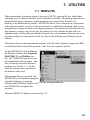
7.1. WINPLOTS . . . . . . . . . . . . . . . . . . . . . . . . . . . . . . . . . . . . . . . . . . . . . . . . . . . . . . . . .
7.1.1. File . . . . . . . . . . . . . . . . . . . . . . . . . . . . . . . . . . . . . . . . . . . . . . . . . . . . . . . . . .
7.1.2. Options . . . . . . . . . . . . . . . . . . . . . . . . . . . . . . . . . . . . . . . . . . . . . . . . . . . . . . .
7.1.2.1. Plot... . . . . . . . . . . . . . . . . . . . . . . . . . . . . . . . . . . . . . . . . . . . . . . . . .
ROI . . . . . . . . . . . . . . . . . . . . . . . . . . . . . . . . . . . . . . . . . . . . . .
Text . . . . . . . . . . . . . . . . . . . . . . . . . . . . . . . . . . . . . . . . . . . . . .
Horizontal . . . . . . . . . . . . . . . . . . . . . . . . . . . . . . . . . . . . . . . . .
Vertical . . . . . . . . . . . . . . . . . . . . . . . . . . . . . . . . . . . . . . . . . . .
7.1.3. Command Line Interface . . . . . . . . . . . . . . . . . . . . . . . . . . . . . . . . . . . . . . . . .
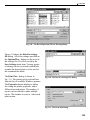
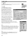
7.2. Nuclide Library Editor . . . . . . . . . . . . . . . . . . . . . . . . . . . . . . . . . . . . . . . . . . . . . . . . .
7.2.1. Copying Nuclides From Library to Library . . . . . . . . . . . . . . . . . . . . . . . . . . .
7.2.2. Creating a New Library Manually . . . . . . . . . . . . . . . . . . . . . . . . . . . . . . . . . .
7.2.3. Editing Library List Nuclides . . . . . . . . . . . . . . . . . . . . . . . . . . . . . . . . . . . . . .
7.2.3.1. Manually Adding Nuclides . . . . . . . . . . . . . . . . . . . . . . . . . . . . . . . .
7.2.3.2. Deleting Nuclides from the Library . . . . . . . . . . . . . . . . . . . . . . . . . .
7.2.3.3. Rearranging the Library List . . . . . . . . . . . . . . . . . . . . . . . . . . . . . . .
7.2.3.4. Editing Nuclide Peaks . . . . . . . . . . . . . . . . . . . . . . . . . . . . . . . . . . . .
7.2.3.5. Adding Nuclide Peaks . . . . . . . . . . . . . . . . . . . . . . . . . . . . . . . . . . . .
7.2.3.6. Rearranging the Peak List . . . . . . . . . . . . . . . . . . . . . . . . . . . . . . . . .
7.2.3.7. Saving or Canceling Changes and Closing . . . . . . . . . . . . . . . . . . . .
7.2.4. Print Library . . . . . . . . . . . . . . . . . . . . . . . . . . . . . . . . . . . . . . . . . . . . . . . . . . .
7.2.5. Close . . . . . . . . . . . . . . . . . . . . . . . . . . . . . . . . . . . . . . . . . . . . . . . . . . . . . . . . .
7.2.6. About... . . . . . . . . . . . . . . . . . . . . . . . . . . . . . . . . . . . . . . . . . . . . . . . . . . . . . . .
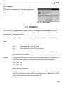
7.3. TRANSLT . . . . . . . . . . . . . . . . . . . . . . . . . . . . . . . . . . . . . . . . . . . . . . . . . . . . . . . . . .
143
143
144
146
146
146
146
147
147
148
148
149
150
151
152
152
152
153
153
153
154
154
154
155
155
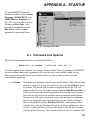
APPENDIX A. STARTUP . . . . . . . . . . . . . . . . . . . . . . . . . . . . . . . . . . . . . . . . . . . . . . . . . . . . 157
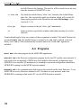
A.1. Command Line Options . . . . . . . . . . . . . . . . . . . . . . . . . . . . . . . . . . . . . . . . . . . . . . . 157
A.2. Programs . . . . . . . . . . . . . . . . . . . . . . . . . . . . . . . . . . . . . . . . . . . . . . . . . . . . . . . . . . . 158
APPENDIX B. FILE FORMATS . . . . . . . . . . . . . . . . . . . . . . . . . . . . . . . . . . . . . . . . . . . . . .
B.1. MAESTRO File Types . . . . . . . . . . . . . . . . . . . . . . . . . . . . . . . . . . . . . . . . . . . . . . . .
B.1.1. Detector Files . . . . . . . . . . . . . . . . . . . . . . . . . . . . . . . . . . . . . . . . . . . . . . . . . .
B.1.2. Spectrum Files . . . . . . . . . . . . . . . . . . . . . . . . . . . . . . . . . . . . . . . . . . . . . . . . .
B.1.3. Miscellaneous Files . . . . . . . . . . . . . . . . . . . . . . . . . . . . . . . . . . . . . . . . . . . . .
viii
159
159
159
159
159
TABLE OF CONTENTS
B.2. Program Examples . . . . . . . . . . . . . . . . . . . . . . . . . . . . . . . . . . . . . . . . . . . . . . . . . . . .
B.2.1. FORTRAN Language . . . . . . . . . . . . . . . . . . . . . . . . . . . . . . . . . . . . . . . . . . .
B.2.1.1. .CHN Files . . . . . . . . . . . . . . . . . . . . . . . . . . . . . . . . . . . . . . . . . . . . .
B.2.1.2. .ROI Files . . . . . . . . . . . . . . . . . . . . . . . . . . . . . . . . . . . . . . . . . . . . .
B.2.2. C Language: . . . . . . . . . . . . . . . . . . . . . . . . . . . . . . . . . . . . . . . . . . . . . . . . . . .
159
160
160
161
162
APPENDIX C. ERROR MESSAGES . . . . . . . . . . . . . . . . . . . . . . . . . . . . . . . . . . . . . . . . . . . 165
INDEX . . . . . . . . . . . . . . . . . . . . . . . . . . . . . . . . . . . . . . . . . . . . . . . . . . . . . . . . . . . . . . . . . . . . 175
ix
NOTE!
We assume that you are thoroughly familiar with 32-bit Microsoft®
Windows® usage and terminology. If you are not fully acquainted
with the Windows environment, including the use of the mouse, we
strongly urge you to read the Microsoft documentation supplied
with your Windows software and familiarize yourself with a few
simple applications before proceeding.
The convention used in this manual to represent actual keys
pressed is to enclose the key label within angle brackets; for
example, <F1>. For key combinations, the key labels are
joined by a + within the angle brackets; for example,
<Alt + 2>.
x
xi
INSTALLATION
If you are installing a new multichannel buffer (MCB) in
addition to MAESTRO-32, or if your MCB and/or new
MAESTRO-32 is accompanied by a CONNECTIONS-32
Driver Update Kit (Part No. 797230), follow the installation
instructions that accompany the driver update kit.
For information on installation and configuration, hardware
driver activation, network protocol configuration, and
building the master list of instruments accessible within
MAESTRO-32, see Chapter 2 (page 7) and the
accompanying ORTEC MCB CONNECTIONS-32 Hardware
Property Dialogs Manual.
xii
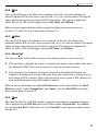
1. INTRODUCTION
Welcome to MAESTRO-32 Version 6. This latest release extends the capabilities of the world's
most popular multichannel analyzer (MCA) emulation software with the addition of a command
that gives you the option of using a multi-detector interface that lets you view up eight MCA
windows and eight buffer windows at a time, or using the “classic,” single-window interface. In
addition, the revised installation wizard provides more guidance in selecting the instrument
drivers you will need. MAESTRO-32 V6 uses the GammaVision library editor so you can now
create, modify, and use both .LIB- and .MDB-format (NuclideNavigator®) libraries. This release
of MAESTRO also supports our new DSPEC Pro™, DSPEC jr 2.0™, Detective™,
Detective-EX™, and trans-SPEC™ instruments.
1.1. MCA Emulation
An MCA, in its most basic form, is an instrument that sorts and counts events in real time. This
sorting is based on some characteristic of these events, and the events are grouped together into
bins for counting purposes called channels. The most common type of multichannel analysis,
and the one which is of greatest interest to nuclear spectroscopists, is pulse-height analysis
(PHA). PHA events are signal pulses originating from a detector.1 The characteristic of interest
is the pulse height or voltage, which is proportional to the particle or photon energy. An analogto-digital converter (ADC) is used to convert each pulse into a channel number, so that each
channel corresponds to a narrow range of pulse heights or voltages. As pulses arrive over time,
the MCA collects in memory a distribution of the number of pulses with respect to pulse height
(a series of memory locations, corresponding to ADC channels, will contain the number of
pulses of similar, although not necessarily identical, height). This distribution, arranged in order
of ascending energies, is commonly referred to as a spectrum. To be useful, the acquired
spectrum must be available for storage and/or analysis, and is displayed on a graph whose
horizontal axis represents the height of the pulse and whose vertical axis represents the number
of pulses at that height, also referred to as a histogram.
MAESTRO-32, combined with multichannel buffer (MCB) hardware and a personal computer,
emulates an MCA with remarkable power and flexibility. The MCB performs the actual pulseheight analysis, while the computer and operating system make available the display facility and
data-archiving hardware and drivers. The MAESTRO software is the vital link that marries these
components to provide meaningful access to the MCB via the user interface provided by the
computer hardware.
The MAESTRO-32 MCA emulation continuously shows the spectrum being acquired, the
current operating conditions, and the available menus. All important operations that need to be
1
In this manual “Detector” (capitalized) means the transducer (high-purity germanium, sodium iodide, silicon
surface barrier, or others) plus all the electronics including the ADC and histogram memory. The transducers are
referenced by the complete name, e.g., high-purity germanium (HPGe) detector.
1
MAESTRO-32® V6 (A65-B32)
performed on the spectrum, such as peak location, insertion of regions of interest (ROIs), and
display scaling and sizing are implemented with both the keyboard (accelerators) and mouse
(toolbar and menus). Spectrum peak searching, report generation, printing, archiving,
calibration, and other analysis tools are available from the menus. Some menu functions have
more than one accelerator so that both new and experienced users will find the system easy to
use. This version of MAESTRO continues to offer the flexibility of constructing automated
sequences or “job streams.”
Buffers are maintained in the computer memory to which one spectrum can be moved for display
and analysis, either from Detector memory or from disk, while another spectrum is collected in
the Detector. As much as possible, the buffer duplicates in memory the functions of the Detector
hardware on which a particular spectrum was collected. Data can also be analyzed directly in the
Detector hardware memory, as well as stored directly from the Detector to disk. This release of
MAESTRO allows you to open up to eight Detector windows and eight buffer windows
simultaneously.
MAESTRO-32 uses the network features of Windows so you can use and control ORTEC MCB
hardware anywhere on the network.
1.2. About This User Manual
This manual is intended to be used in conjunction with the ORTEC MCB CONNECTIONS-32
Hardware Property Dialogs Manual (Part No. 931001, hereinafter called the “MCB Properties
manual”) included with MAESTRO. The hardware property dialogs manual contains the
hardware setup information for our CONNECTIONS-compliant MCBs (these dialogs are discussed
in more detail in Section 4.2.7). In addition, it provides detailed instructions on installing
CONNECTIONS software, building the Master Instrument List of all ORTEC MCBs connected to
your PC locally and across a network, and selecting the proper protocol for communicating with
networked ORTEC instruments.
1.3. PC Requirements
MAESTRO-32 (A65-B32) is designed for use on PCs that run Microsoft Windows 98 SE, 2000
Pro, and XP Pro. For PCs with a memory-mapped MCB interface, no other interface can use
memory mapped into page D of the PC memory map (see the MCB Properties manual). Data can
be saved or retrieved from any number of removable or fixed drives.
2
1. INTRODUCTION
1.4. Detectors
Front-end acquisition hardware supported includes ORTEC’s CONNECTIONS-32-compliant
MCBs interfaced to the computer with an appropriate adapter card and cable, or using the
printer-port adapter. In a network, the ORSIM™ III can also be used to connect MCBs directly to
the Ethernet.
MAESTRO-32 can control and display an almost unlimited number of Detectors, either local or
networked; the limit depends on system resources. These can be any mixture of the following
types of units, properly installed and hardware-configured: DSPEC Pro™, DSPEC jr 2.0™,
Detective™, Detective-EX™, trans-SPEC™, digiBASE™, microBASE™, DSP-Scint™,
digiDART™, DSPEC Plus™, DSPEC jr™, Models 916A, 917, 918A, 919, 920, 921, 926, 919E,
920E, 921E, 92X, 92X-II, NOMAD™ Plus, NOMAD, MicroNOMAD®, OCTÊTE® PC,
TRUMP™, MicroACE™, DART®, DSPEC, MatchMaker™, M3CA, MiniMCA-166, and other new
modules. MAESTRO-32 will correctly display and store a mixture of different sizes of spectra.
Multiple MAESTRO windows can be open at one time, displaying Detectors, buffers, spectrum
files from disk, and data analyses. The larger and higher-resolution your monitor, the more
windows you can comfortably view.
Expanding the system for more Detectors (as well as enabling more than one device on a
Model 919) is easy. When the system incorporates a Model 920- or OCTÊTE PC-type MCB, the
system can also be expanded using the internal multiplexer/router. In the Model 920 or
OCTÊTE PC, the MCB memory is divided into segments so that each input has an equal share of
the MCB memory, the size of which matches the conversion gain or maximum channel number
of the ADC. Note that in the multiple-input MCBs like the Model 919 or Model 920, all inputs
are treated as different Detectors. Therefore, all CONNECTIONS software will address one
physical 919 unit as four distinct Detectors.
1.5. Detector Security
Detectors can be protected from destructive access by password. If your application supports
detector locking and unlocking, passwords can be set within the application. Once a password is
set, no application can start, stop, clear, change presets, change ROIs, or perform any command
that affects the data in the detector if the password is not known. The current spectrum and
settings for the locked device can be viewed read-only. The password is required for any
destructive access, even on a network. This includes changing instrument descriptions and IDs
with the MCB Configuration program.
3
MAESTRO-32® V6 (A65-B32)
1.6. Enhancements to MAESTRO for Windows
1.6.1. MAESTRO-32 V6.04 vs. V6
1. The new Multiple Windows command, on the Window menu, lets you choose between the
newer multiple-detector-window mode and the original single-detector-window mode.
2. MAESTRO no longer supports operation with Microsoft Windows 95, NT or the earliest
release of Windows 98 (as distinguished from Windows 98 Second Edition, which is still
supported).
3. Support has been added for the new ORTEC DSPEC Pro, DSPEC jr 2.0, Detective,
Detective-EX, and trans-SPEC MCBs.
1.6.2. MAESTRO-32 V6 vs. V5.35
1. MAESTRO now has a multi-detector interface that allows you to open up to eight Detector
windows and eight buffer windows simultaneously.
2. Support has been added for the new ORTEC digiBASE, microBASE, and DSP-Scint MCBs.
3. The list of library peaks can be sorted by clicking on the column header.
4. MAESTRO now uses the same library editor as GammaVision-32®, so both .LIB- and .MDBformat libraries can be created, modified, and used within the program. The old MAESTRO
.MCA library file format is no longer supported.
1.6.3. MAESTRO-32 V5.35 vs. V5.3
1. Support for Windows XP Pro has been added.
2. Operation with Windows 95 is not guaranteed.
3. The DSPEC jr is supported on the USB port.
4. Support for SP3 of Windows 2000 has been added.
1.6.4. MAESTRO-32 V5.3 vs. V5.
1. The digiDART portable MCA is supported on the USB port.
2. The MCB presets and controls have been moved into a single menu control, MCB
Properties. This makes all the MCB controls more uniform and more in line with other
Windows programs.
4
1. INTRODUCTION
3. Isotope markers have been added. The isotope markers show all the gamma rays of a single
nuclide (from the library) on the spectrum displays when any one of the gamma rays from
that nuclide is selected on the spectrum. The amplitude of the marker for the selected peak is
proportional to the peak area. The amplitude of the marker for the other peaks is proportional
to the first peak and the branching ratio.
4. Support for the SBS60 has been added. The SBS60 is a single ISA card spectrometer
intended for use in Safeguards applications.
5. Support for Windows 2000 Pro has been added.
5
MAESTRO-32® V6 (A65-B32)
6
2. INSTALLING MAESTRO-32
If your MAESTRO CD is accompanied by a CONNECTIONS-32 Driver Update Kit (Part No.
797230), follow the installation instructions that accompany the update kit, which supersede the
instructions below.
NOTE For systems using Windows 2000 or XP, ORTEC CONNECTIONS-32 software products
are designed to operate correctly only for users with full Administrator privileges.
Limiting user privileges could cause unexpected results.
1) Insert the MAESTRO-32 CD. If it does not autorun, go to the Windows Taskbar and click on
Start, then Run.... In the Run dialog, enter D:\Disk 1\Setup.exe (use your CD-ROM
drive designator instead of D:), then click on OK. This will start the installation wizard; click
on Next and follow the wizard prompts.
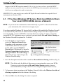
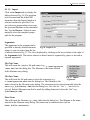
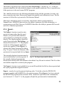
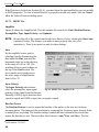
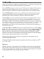
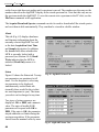
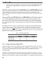
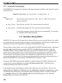
2) On the Instrument Setup page, mark the checkbox(es) that corresponds to the instrument(s)
installed on your PC, as shown in Fig. 1. To see more information on each instrument family,
click on the family name and read the corresponding Item Description on the right side of
the dialog.
If this is a MAESTRO upgrade and not a first-time installation, you probably already have
ORTEC CONNECTIONS-32 instruments attached to your PC. If so, they will be included on
the Local Instrument List at the bottom of the dialog, along with any new instruments.
Existing (previously configured before this upgrade) instruments do not have to be powered
on during this part of the installation procedure.
NOTE You can enable other device drivers later, as described in Section 2.2.
3) If you want other computers in a network to be able to use your MCBs, leave the Allow
other computers to use this computer’s instruments marked so the MCB Server program
will be installed. Most users will leave this box marked for maximum flexibility.
NOTE If your PC uses Windows XP and you wish to use or share ORTEC MCBs across a
network, be sure to read Section 2.1.
4) Click on Done.
If your PC is operating under Windows 2000 or XP, the installation wizard will resume
copying files.
7
MAESTRO-32® V6 (A65-B32)
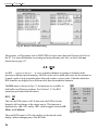
Fig. 1. Choose the Interface for Your Instruments.
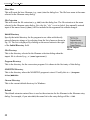
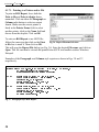
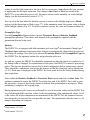
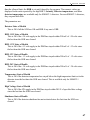
If your PC uses Windows 98 SE, two additional dialogs might be displayed. The first, shown
in Fig. 2, might ask you to insert the “ORTEC Installation CD”. Ignore this message and
click on OK.
Fig. 2. Window Menu.
8
2. INSTALLING MAESTRO-32
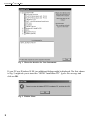
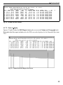
The second additional dialog could request a specific file (see the example in Fig. 3). Browse
to the c:\Program Files\Common Files\ORTEC Shared\UMCBI folder (not to the
MAESTRO CD), then click on OK. The installation wizard will resume copying files.
Fig. 3. Window Menu.
5) At the end of the wizard, restart the PC. Upon restart, remove the MAESTRO CD from the
drive.
6) After all processing for new plug-and-play devices has finished, you will be ready to
configure the MCBs in your system. Connect and power on all local and network ORTEC
instruments that you wish to use, as well as their associated PCs. Otherwise, the software will
not detect them during installation. Any instruments not detected can be configured at a later
time.
7) If any of the components on the network is a DSPEC Plus, ORSIM II or III, MatchMaker,
9DSPEC, 92X-II, 919E, 920E, 921E, or other module that uses an Ethernet connection, the
network default protocol must be set to the IPX/SPX Compatible Transport with NetBIOS
selection on all PCs that use CONNECTIONS hardware. For instructions on making this the
default, see the network protocol setup discussion in the MCB Properties Manual..
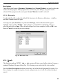
8) To start the MCB Configuration program on your PC, click on Start, Programs,
MAESTRO 32, and MCB Configuration. Alternatively, you can go to c:\Program
Files\Common Files\ORTEC Shared\Umcbi and run MCBCON32.EXE. The MCB
Configuration program will locate all of the (powered-on) ORTEC MCBs attached to the
local PC and to (powered-on) network PCs, display the list of instruments found, allow you
to enter customized instrument numbers and descriptions, and optionally write this
configuration to those other network PCs, as described in detail in the software installation
9
MAESTRO-32® V6 (A65-B32)
chapter of the MCB Properties manual. If this is the first time you have installed ORTEC
software on your system, be sure to refer to the MCB Properties manual for information on
initial system configuration and customization.
MAESTRO-32 is now ready to use, and its MCB pick list can be tailored to a specific list of
instruments (see Section 4.4.5).
2.1. If You Have Windows XP Service Pack 2 and Wish to Share
Your Local ORTEC MCBs Across a Network
NOTE If you do not have instruments connected directly to your PC or do not wish to share
your instruments, this section does not apply to you.
If you have installed Windows XP Service Pack 2 and have fully enabled the Windows Firewall,
as recommended by Microsoft, the default firewall settings will prevent other computers from
accessing the CONNECTIONS-32 MCBs connected directly to your PC. To share your locally
connected ORTEC instruments across a network, you must enable File and Printer Sharing on
the Windows Firewall Exceptions list. To do this:
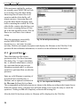
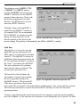
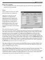
1. From the Windows Control Panel,
access the Windows Firewall entry.
Depending on the appearance of your
Control Panel, there are two ways to
do this. Either open the Windows
Firewall item (if displayed); or open the
Network Connections item then choose
Change Windows Firewall Settings, as
illustrated in Fig. 4. This will open the
Windows Firewall dialog.
Fig. 4. Change the Firewall Settings.
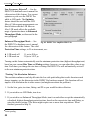
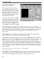
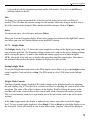
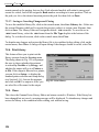
2. Go to the Exceptions tab, then click to mark the File and Printer Sharing checkbox (Fig. 5).
NOTE This affects only the ability of other users on your network to access your MCBs.
You are not required to turn on File and Printer Sharing in order to access
networked MCBs (as long as those PCs are configured to grant remote access).
3. To learn more about exceptions to the Windows Firewall, click on the What are the risks of
allowing exceptions link at the bottom of the dialog.
4. Click on OK to close the dialog. No restart is required.
10
2. INSTALLING MAESTRO-32
Fig. 5. Turn on File and Printer Sharing.
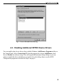
2.2. Enabling Additional ORTEC Device Drivers
You can enable other device drivers later with the Windows Add/Remove Programs utility on
the Control Panel. Select Connections 32 from the program list, choose Add/Remove, then
elect to Modify the software setup. This will reopen the Instrument Setup dialog so you can
mark or unmark the driver checkboxes as needed, close the dialog, then re-run the MCB
Configuration program as described in Step 8 on page 9.
11
MAESTRO-32® V6 (A65-B32)
12
3. GETTING STARTED
This chapter tells how to start MAESTRO, explains its display features, discusses the role of the
mouse and keyboard, covers the use of the Toolbar and sidebars, discusses how to change to
different disk drives and folders, and shows how to use additional features such as Help.
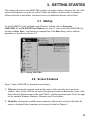
3.1. Startup
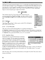
To start MAESTRO, click on Start on the Windows Taskbar, then on Programs,
MAESTRO 32, and MAESTRO for Windows (see Fig. 6). You can also start MAESTRO by
clicking on Start, Run..., and entering a command line in the Run dialog, with or without
arguments, as described in Section A.1.
Fig. 6. Starting MAESTRO.
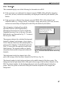
3.2. Screen Features
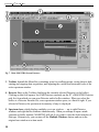
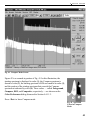
Figure 7 shows MAESTRO’s principal screen features:
1. Title bar, showing the program name and the source of the currently active spectrum
window. There is also a title bar on each of the spectrum windows showing the source of the
data: either the Detector name or the word “Buffer” with the spectrum name. On the far right
are the standard Windows Minimize, Maximize, and Close buttons.
2. Menu Bar, showing the available menu commands (which can be selected with either the
mouse or keyboard); these functions are discussed in detail in Chapter 4.
13
MAESTRO-32® V6 (A65-B32)
Fig. 7. Main MAESTRO Screen Features.
3. Toolbar, beneath the Menu Bar, containing icons for recalling spectra, saving them to disk,
starting and stopping data acquisition, and adjusting the vertical and horizontal scale of the
active spectrum window.
4. Detector List, on the Toolbar, displaying the currently selected Detector (or the buffer).
Clicking on this field opens a list of all Detectors currently on the PC’s MAESTRO Detector
pick list, from which you can open Detector and/or buffer windows. When you select the
buffer or a Detector from the list, a new spectrum window opens, to a limit of eight. If you
selected a Detector, the spectrum in its memory (if any) is displayed.
5. Spectrum Area, which displays multiple spectrum windows — up to eight Detector
windows and eight buffer windows simultaneously. When you attempt to open a ninth
spectrum or buffer window, MAESTRO will ask if you wish to close the oldest window of
that type. Alternatively, you can turn off the Multiple Windows feature and run in the
original one-window-at-a-time mode.
14
3. GETTING STARTED
Spectrum windows can be moved, sized, minimized, maximized, and closed with the mouse,
as well as tiled horizontally or vertically from the Window menu. When more than one
window is open, only one is active — available for data manipulation and analysis — at a
time. The title bar on the active window will normally be a brighter color than those on the
inactive windows (the color scheme will depend on the desktop colors you have selected in
Windows Control Panel). Detector windows or buffer windows containing a spectrum from
an MCB will list the Detector name on the title bar. If you have opened a spectrum file into a
buffer window, the title bar will display the filename. To switch windows, click on the
window that you wish to activate, use the Window menu (see Section 4.7), or cycle between
windows by pressing <Ctrl + Tab>.
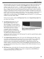
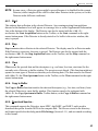
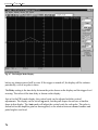
Each spectrum window contains a Full Spectrum View and an Expanded Spectrum View
(see items 6 and 7 below).
6. The Full Spectrum View shows the
full histogram from the file or the
Detector memory. The vertical scale is
always logarithmic, and the window can
be moved and sized (see Section 3.5.4).
The Full Spectrum View contains a
Fig. 8. Contents of Expanded Spectrum View are
rectangular window that marks the
Highlighted in Full Spectrum View.
portion of spectrum now displayed in
the Expanded Spectrum View (see Fig. 8).
To quickly move to different part of the
spectrum, just click on that area in the Full Spectrum View and the expanded display updates
immediately at the new position.
7. The Expanded Spectrum View shows all or part of the full histogram; this allows you to
zoom in on a particular part of the spectrum and see it in more detail. You can change the
expanded view vertical and horizontal scaling, and perform a number of analytical
operations such as peak information, marking ROIs, or calibrating the spectrum. This
window contains a vertical line called a marker that highlights a particular position in the
spectrum. Information about that position is displayed on the Marker Information Line (see
item 10 below).
8. ROI Status Area, on the right side of the menu bar, indicates whether the ROI marking
mode is currently Mark or UnMark. This operates in conjunction with the ROI menu
commands and arrow keys (see Section 4.5).
15
MAESTRO-32® V6 (A65-B32)
9. Status Sidebar, on the right side of the screen, provides information on the current Detector
presets and counting times, the time and date, and a set of buttons for moving easily between
peaks, ROIs, and library entries (see Section 3.6).
10. Marker Information Line, beneath the spectrum, showing the marker channel, marker
energy, and channel contents.
11. Supplementary Information Line, below the Marker Information Line, used to show
library contents, the results of certain calculations, warning messages, or instructions.
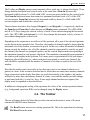
3.3. Spectrum Displays
The Full and Expanded Spectrum Views show, respectively, a complete histogram of the current
spectrum (whether from a Detector or the buffer) and an expanded view of all or part of the
spectrum. These two windows are the central features of the MAESTRO screen. All other
windows and most functions relate to the spectrum windows. The Full Spectrum View shows the
entire data memory of the Detector as defined in the configuration. In addition, it has a marker
box showing which portion of the spectrum is displayed in the Expanded Spectrum View.
The Expanded Spectrum View contains a reverse-color marker line at the horizontal position of
the pixel representing the marker channel. This marker can be moved with the mouse pointer, as
described in Section 3.5.1, and with the <7
7>/<6
6> and <PgUp>/<PgDn> keys.
Note that in both spectrum windows the actual spectrum is scaled to fit in its window as it
appears on the display. Also, since both windows can be arbitrarily resized (a feature of
Windows), it follows that the scaling is not always by powers of two, nor even integral
multiples. Therefore, MAESTRO uses algorithms to scale the window properly and maintain the
correct peak shapes regardless of the actual size of the window. The vertical scale in the Full
Spectrum View is always logarithmic. In the Expanded Spectrum View, use the menus, rightmouse-button menu, accelerator keys, and Toolbar to choose between logarithmic and linear
scales, change both axis scales by zooming in and out, and select which region of the spectrum
to view.
The spectrum display can be expanded to show more detail or contracted to show more data
using the Zoom In and Zoom Out features.2 Zooming in and out can be performed using the
Toolbar buttons, the Display menu commands, or the rubber rectangle (see Section 3.5.3). The
rubber rectangle allows the spectrum to be expanded to any horizontal or vertical scale. The
baseline or “zero level” at the bottom of the display can also be offset with this tool, allowing
the greatest possible flexibility in showing the spectrum in any detail.
2
These replace the Narrower/Wider and Shorter/Taller commands in older versions of MAESTRO.
16
3. GETTING STARTED
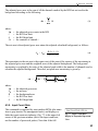
The Toolbar and Display menu zoom commands offer a quick way to change the display. These
change both the horizontal and vertical scales at the same time. Zoom In decreases the
horizontal width by about 6% of full width (ADC conversion gain) and halves the vertical scale.
The Zoom In button and menu item zoom to a minimum horizontal scale of 6% of the ADC
conversion gain. Zoom Out increases the horizontal width by about 6% of full width (ADC
conversion gain) and doubles the vertical scale.
The accelerator keys have also changed. Keypad<+> and Keypad<!
!>, respectively, duplicate
the Zoom In and Zoom Out Toolbar buttons and Display menu commands. The <F5>/<F6>
and <9
9>/<8
8> keys change the vertical scale by a factor of two without changing the horizontal
scale. The <F7>/<F8> and keyboard <!
!>/<+> keys change the horizontal scale by a factor of
two without changing the vertical scale.
Depending on the expansion or overall size of the spectrum, all or part of the selected spectrum
can be shown in the expanded view. Therefore, the number of channels might be larger than the
horizontal size of the window, as measured in pixels. In this case, where the number of channels
shown exceeds the window size, all of the channels cannot be represented by exactly one pixel
dot. Instead, the channels are grouped together, and the vertical displacement corresponding to
the maximum channel in each group is displayed. This maintains a meaningful representation of
the relative peak heights in the spectrum. For a more precise representation of the peak shapes
displaying all available data (i.e., where each pixel corresponds to exactly one channel), the
scale should be expanded until the number of channels is less than or equal to the size of the
window.
Note that the marker can be moved by no less than one pixel or one channel (whichever is
greater) at a time. In the scenario described above, where there are many more memory channels
being represented on the display than there are pixels horizontally in the window, the marker
will move by more than one memory channel at a time, even with the smallest possible change
as performed with the <6
6> and <7
7> keys. If true single-channel motions are required, the
display must be expanded as described above.
In addition to changing the scaling of the spectrum, the colors of the various spectrum features
(e.g., background, spectrum, ROIs) can be changed using the Display menu.
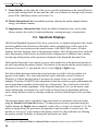
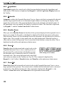
3.4. The Toolbar
The row of buttons below the Menu Bar provides convenient shortcuts to some of the most
common MAESTRO menu functions.
The Recall button retrieves an existing spectrum file. This is the equivalent of selecting
File/Recall from the menu.
17
MAESTRO-32® V6 (A65-B32)
Save copies the currently displayed spectrum to disk. It duplicates the menu functions
File/Save or File/Save As... (depending on whether the spectrum was recalled from disk,
and whether any changes have been made to the spectrum window since the last save).
Start Acquisition starts data collection in the current Detector. This duplicates
Acquire/Start and <Alt + 1>.
Stop Acquisition stops data collection. This duplicates Acquire/Stop and <Alt + 2>.
Clear Spectrum clears the detector or file spectrum from the window. This duplicates
Acquire/Clear and <Alt + 3>.
Mark ROI automatically marks an ROI in the spectrum at the marker position, according
to the criteria in Section 4.5.4. This duplicates ROI/Mark Peak and <Insert>.
Clear ROI removes the ROI mark from the channels of the peak currently selected with
the marker. This duplicates ROI/Clear and <Delete>.
The next section of the Toolbar (Fig. 9) contains the buttons that control the
spectrum’s vertical scale. These commands are also on the Display menu. In
addition, vertical scale can be adjusted by zooming in with the mouse (see
Fig. 15).
Fig. 9. Vertical
Scaling Section of
Toolbar.
Vertical Log/Lin Scale switches between logarithmic and linear
scaling. When switching from logarithmic to linear, it uses the previous linear scale
setting. Its keyboard duplicate is Keypad</>.
Vertical Auto Scale turns on the autoscale mode, a linear scale that automatically adjusts
until the largest peak shown is at its maximum height without overflowing the display. Its
keyboard duplicate is Keypad<*>.
The field to the left of these two buttons displays LOG if the scale is logarithmic, or indicates
the current vertical full-scale linear value.
The horizontal scaling section (Fig. 10) follows next. It includes a
field that shows the current window width in channels, and the
Zoom In, Zoom Out, Center, and Baseline Zoom buttons. These
commands are also on the Display menu. In addition, horizontal
scale can be adjusted by zooming in with the mouse (see Fig. 15).
18
Fig. 10. Horizontal Scaling
Section of Toolbar.
3. GETTING STARTED
Zoom In decreases the horizontal full scale of the Expanded Spectrum View according to
the discussion in Section 3.3, so the peaks appear “magnified.” This duplicates
Display/Zoom In and Keypad<+>.
Zoom Out increases the horizontal full scale of the Expanded Spectrum View according
to the discussion in Section 3.3, so the peaks appear reduced in size. This duplicates
Display/Zoom Out and Keypad<!
!>.
Center moves the marker to the center of the screen by shifting the spectrum without
moving the marker from its current channel. This duplicates Display/Center and
Keypad<5>.
Baseline Zoom keeps the baseline of the spectrum set to zero counts.
The right-most part of the Toolbar is a drop-down list of the available Detectors (Fig. 11). To
select a Detector or the buffer, click in the field or on the down-arrow beside it to open the list,
then click on the desired entry. The sidebar will register your selection.
Finally, note that as you pause the mouse pointer over the center of a Toolbar button, a pop-up
tool tip box opens, describing the button’s function (Fig. 12).
Fig. 12. Tool Tip.
Fig. 11. Drop-Down
Detector List.
3.5. Using the Mouse
The mouse can be used to access the menus, Toolbar, and sidebars; adjust spectrum scaling;
mark and unmark peaks and ROIs; select Detectors; work in the dialogs — every function in
MAESTRO except text entry. For most people, this might be more efficient than using the
keyboard. The following sections describe specialized mouse functions.
19
MAESTRO-32® V6 (A65-B32)
3.5.1. Moving the Marker with the Mouse
To position the marker with the mouse, move the pointer to the desired channel in the Expanded
Spectrum View and click the left mouse button once. This will move the marker to the mouse
position. This is generally a much easier way to move the marker around in the spectrum than
using the arrow keys, although you might prefer to use the keys for specific motions (such as
moving the marker 1 channel at a time).
3.5.2. The Right-Mouse-Button Menu
Figure 13 shows the right-mouse-button menu. To open it, position the
mouse pointer in the spectrum display, click the right mouse button, then
use the left mouse button to select from its list of commands. Not all of the
commands are available at all times, depending on the spectrum displayed
and whether the rubber rectangle is active. Except for Undo Zoom In, all
of these func-tions are on the Toolbar and/or the Menu Bar (Peak Info
and Sum are only on the Menu Bar, under Calculate). See Section 4.8 for
more information on the commands.
3.5.3. Using the “Rubber Rectangle”
The rubber rectangle is used for selecting a particular area of interest
within a spectrum. It can be used in conjunction with the right-mousebutton menu in Fig. 13 for many functions. To draw a rubber rectangle:
1. Click and hold the left mouse button; this anchors the starting corner
of the rectangle.
Fig. 13. RightMouse-Button Menu
for Spectra.
2. Drag the mouse diagonally across the area of interest. As you do this,
the mouse will be drawing a reverse-color rectangle bisected by the
marker line. Note that when drawing a rubber rectangle, the marker
line combines with a horizontal line inside the rectangle to form
crosshairs (Fig. 14). They make it easy to select the center channel in
the area of interest — this might be the center of an ROI that you
wish to mark or unmark, a portion of the spectrum to be summed, or
a peak for which you want detailed information.
3. Release the mouse button; this anchors the ending corner of
the rectangle.
20
Fig. 14. The Rubber
Rectangle’s
Crosshairs.
3. GETTING STARTED
4. Click the right mouse button to open its menu, and select one of the available commands.
Once an area is selected, the commands can also be issued from the Toolbar, Menu Bar,
Status Sidebar, or keyboard.
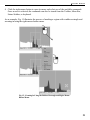
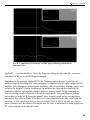
As an example, Fig. 15 illustrates the process of marking a region with a rubber rectangle and
zooming in using the right-mouse-button menu.
Fig. 15. Zooming In Using the Rubber Rectangle and Right-MouseButton Menu.
21
MAESTRO-32® V6 (A65-B32)
3.5.4. Sizing and Moving the Full Spectrum View
To change the horizontal and vertical size of the
Full Spectrum View, move the mouse pointer onto
the side edge, bottom edge, or corner of the window
until the pointer changes to a double-sided arrow
(see Fig. 16). Click and hold the left mouse button,
drag the edge of the window until it is the size you
want, then release the mouse button.
To move the Full Spectrum View to a different part
of the screen, move the mouse pointer onto the top
edge of the window until the pointer changes to
a four-sided arrow (see Fig. 16). Click and hold the
left mouse button, drag the window to its new
location, and release the mouse button.
Fig. 16. Two-Sided Pointer for Sizing Full
Spectrum View, and Four-Sided Pointer for
Moving Window.
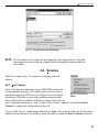
3.6. Buttons and Boxes
This section describes MAESTRO’s radio buttons, indexing buttons,
and checkboxes. To activate a button or box, just click on it.
Radio buttons (Fig. 17) appear on many MAESTRO dialogs, and
allow only one of the choices to be selected.
Fig. 17. Radio Buttons.
Checkboxes (Fig. 18) are another common feature, allowing one or
more of the options to be selected at the same time.
The ROI, Peak, and Library indexing buttons on the Status Sidebar
are useful for rapidly locating ROIs or peaks, and for advancing between
entries in the library. When the last item in either direction is reached,
the computer beeps and MAESTRO posts a “no more” message on the
Supplementary Information Line. If a library file has not been loaded or
the Detector is not calibrated, the Library buttons are disabled and shown
in gray.
Fig. 18. Checkboxes.
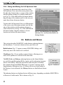
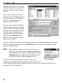
The indexing buttons are displayed in two different ways, depending on whether MAESTRO is
in Detector or buffer mode. This is shown in Fig. 19.
22
3. GETTING STARTED
In Detector mode, the buttons appear at the bottom of the Status Sidebar.
In buffer mode, the buttons are overlaid where the Presets and indexing
buttons are displayed in Detector mode.
The ROI, Peak, and Library buttons function the same in both modes. In
buffer mode, the additional features are the ability to insert or delete an
ROI with the Ins and Del buttons, respectively (located between the ROI
indexing buttons); and to display the peak information for an ROI with the
Info button (located between the Peak indexing arrows).
The Library buttons are useful after a peak has been located to advance
forward or backward through the library to the next closest library entry.
Each button press advances to the next library entry and moves the marker
to the corresponding energy.
Instead of using the Peak buttons to index from a previously identified
peak, position the marker anywhere in the spectrum and click on the
Library buttons to locate the entries closest in energy to that point. If a
warning beep sounds, it means that all library entries have been exhausted
in that direction, or that the spectrum is not calibrated. In any case, if an
appropriate peak is available at the location of the marker, data on the peak
are displayed on the Marker Information Line at the bottom of the screen.
Fig. 19. Indexing
Buttons (Detector
mode, top; buffer
mode, bottom).
The ROI and Peak indexing buttons are duplicated by <Shift+ 7>/
<Shift+ 6> and <Ctrl+ 7>/ <Ctrl+ 6>, respectively. The Library buttons are duplicated by
<Alt+ 7>/<Alt+ 6>. The Del button function is duplicated by the <Delete> key and Clear ROI
on the menus and Toolbar. The Ins button has the same function as the <Insert> key and Mark
ROI on the menus and Toolbar. The Info button duplicates the Calculate/Peak Info command,
Peak Info on the right-mouse-button menu, and double-clicking in the ROI.
3.7. Opening Files with Drag and Drop
Several types of files can be selected and loaded into MAESTRO using the Windows drag-anddrop feature. The file types are: spectra (.SPC, .AN1, .CHN), library (.LIB), and region of
interest (.ROI).
The drag-and-drop file is handled the same as a read (recall) operation for that type of file. For
spectra, this means a buffer window is opened, the file is loaded into it, and the spectrum is
displayed. Library files become the working library files. The ROIs saved in an .ROI file are
read and the regions set.
23
MAESTRO-32® V6 (A65-B32)
To drag and drop, open MAESTRO and Windows Explorer, and display both together on the
screen. Locate a file in Explorer such as DEMO.CHN. Now click and hold the left mouse button,
move the mouse (along with the file “ghost”) to the MAESTRO window, and release the mouse
button. The spectrum file will open as if you had recalled it from within MAESTRO.
3.8. Associated Files
When MAESTRO is installed, it registers the spectrum files in Windows so they can be opened
from Windows Explorer by double-clicking on the filename. The spectrum files are displayed in
WINPLOTS. These files are marked with a spectrum icon ( ) in the Explorer display. The
.JOB files ( ) are also registered, and open in Windows Notepad.
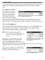
3.9. Editing
Many of the text entry fields in the MAESTRO dialogs support the Windows
editing functions on the right-mouse-button menu. Use these functions to copy
text from field to field with ease, as well as from program to program. Position
the mouse pointer in the text field and click the right mouse button to open the
menu shown in Fig. 20. Select a function from the menu with the left mouse
button.
Fig. 20. RightMouse-Button
Menu for
Dialogs.
24
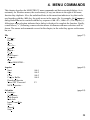
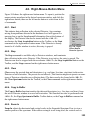
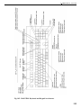
4. MENU COMMANDS
This chapter describes the MAESTRO-32 menu commands and their associated dialogs. As is
customary for Windows menus, the accelerator(s) (if any) are shown to the right of the menu
function they duplicate. Also, the underlined letter in the menu item indicates a key that can be
used together with the <Alt> key for quick access in the menu. (So, for example, the Compare...
dialog under File can be reached with the key sequence <Alt + F>, <Alt + C>.) The ellipsis (...)
following a menu selection indicates that a dialog is displayed to complete the function. Finally,
a small arrow (“<”) following a menu selection means a submenu with more selections will be
shown. The menus and commands covered in this chapter, in the order they appear on the menu
bar, are:
File
Settings...
Recall...
Save
Save As...
Export...
Import...
Print...
ROI Report...
Compare...
Exit
About MAESTRO...
(page 27)
Acquire
Start
Stop
Clear
Copy to Buffer
Download Spectra
View ZDT Corrected
MCB Properties...
(page 42)
Calculate
Settings...
Calibration...
Peak Search
Peak Info
Input Count Rate
Sum
Smooth
Strip...
Alt+1
Alt+2
Alt+3
Alt+5
F3
(page 84)
25
MAESTRO-32® V6 (A65-B32)
(page 91)
Services
JOB Control...
Library file <
Select Peak
Select File
Sample Description...
Lock/Unlock Detector...
Edit Detector list...
ROI
Off
Mark
UnMark
Mark Peak
Clear
Clear All
Save File...
Recall File...
Display
Detector...
Detector/Buffer
Logarithmic
Automatic
Baseline Zoom
Zoom In
Zoom Out
Center
Full View
Isotope Markers
Preferences <
Points
Fill ROI
Fill All
Spectrum Colors...
Peak Info Font/Color...
26
(page 96)
F2 or Alt+O
F2 or Alt+M
F2 or Alt+U
Insert
Delete
(page 99)
Ctrl+<Fn>
F4 or Alt+6
Keypad( / )
Keypad( * )
Keypad( + )
Keypad( - )
Keypad( 5 )
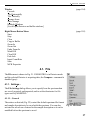
3. MENU COMMANDS
Window
Cascade
Tile Horizontally
Tile Vertically
Arrange Icons
Auto Arrange
Multiple Windows
[List of open Detector and buffer windows]
(page 104)
Right-Mouse-Button Menu
Start
Stop
Clear
Copy to Buffer
Zoom In
Zoom Out
Undo Zoom In
Mark ROI
Clear ROI
Peak Info
Input Count Rate
Sum
MCB Properties
(page 105)
4.1. File
The File menu is shown in Fig. 21. If MAESTRO is in Detector mode
and the selected Detector is acquiring data, the Compare... command is
disabled (gray).
4.1.1. Settings...
The File Settings dialog allows you to specify how the spectrum data
are saved, exported, and imported; and to set the directories for file
types used by MAESTRO.
4.1.1.1. General
The entries on this tab (Fig. 22) control the default spectrum file format
and sample description to be saved with the spectrum. You can also
activate the ask-on-save feature for the sample description so it can be
modified before the spectrum is saved.
Fig. 21. File Menu.
27
MAESTRO-32® V6 (A65-B32)
When you finish setting the parameters
in this dialog and click on OK, these
settings will be used until changed.
The file types are integer .CHN,
integer.SPC floating-point .SPC, and
ASCII .SPE. The .CHN file format is
the format used by all versions of
MAESTRO. It is the simplest format
and, therefore, the easiest to read with
other programs. It does not contain the
analysis parameter data, the complete
calibration, or other data needed for
the nuclide analysis. The format is
described in the ORTEC Software
Fig. 22. General Tab.
File Structure Manual for DOS and
Windows® Systems (Part No. 753800,
hereinafter called the “File Structure Manual”).
The two .SPC formats, integer and floating-point, are identical except for the format of the
spectrum data. The integer .SPC format should be used unless the files are to be used by earlier
versions of ORTEC programs. The .SPC files written by MAESTRO contain the energy
calibration data and the hardware parameters. The integer format stores the spectrum as 4-byte
integers and the floating-point format uses the 4-byte exponential format used in the hardware
math coprocessor (e.g., 80387) and most languages for the PC. The analysis and calibration
formats are defined in the File Structure Manual.
Sample Description allows you to designate the default sample description to be saved with the
spectrum (128-character maximum for .SPC files; 63 characters for .CHN files). If you also mark
the corresponding Ask on Save checkbox, this description will be presented for acceptance or
modification when the spectrum is saved. This is a time-saver that lets you enter the common
descriptors for a group of samples ahead of time then add the unique descriptors on a
sample-by-sample basis after acquisition.
4.1.1.2. Export
Click on the Export tab to display the screen shown in Fig. 23. The program, arguments, and
file directory to be used when the Export function is selected are specified here.
28
3. MENU COMMANDS
Choose any program3 that can accept
the spectrum filename as an argument
on the command line. Use the
Browse... button to automatically
select the complete proper path for the
program.
Arguments
The Arguments to the program
can be specified as directly entered
character strings or you can select
from the list of “macros” shown in
Fig. 24. The list is displayed by
clicking on the arrow button
Fig. 23. Export Tab.
to the right of the Arguments field.
Entries (macros or direct) must be separated by spaces to be read as separate arguments.
File Path Name
This will insert the complete file pathname (e.g., c:\user\spectrum\test.chn) into the dialog
box. The filename is the name selected in the filename entry dialog.
File Base Name
This will insert the file path name without the extension (e.g.,
c:\user\spectrum\test) into the dialog box. The filename is the
name selected in the filename entry dialog. The extension can be
entered manually after the macro (e.g., $(FullBase).CHN) into the
dialog box. Note that the “dot” ( . ) must also be entered. Related
filenames can also be made by adding characters before the “dot”
(e.g., $(FullBase)A.CHN).
Fig. 24. Export
Argument Macros.
Short Name
This will insert the filename (e.g., test.CHN) into the dialog box. The filename is the name
selected in the filename entry dialog. File names can be constructed as $(file
base).$(file extension).
3
Any executable program that can be executed from the Windows Run command can be selected, including DOS
batch commands.
29
MAESTRO-32® V6 (A65-B32)
Short Base
This will insert the base filename (e.g., test) into the dialog box. The file base name is the name
selected in the filename entry dialog.
File Extension
This will insert the file extension (e.g., CHN) into the dialog box. The file extension is the name
selected in the filename entry dialog. Note that the “dot” is not included. Any manually inserted
input of the macro form ($(xxx)) will be included in the argument list without changes.
Initial Directory
The initial directory for the program to use can be specified as directly
entered character strings or the user can select from the list of macros in
Fig. 25. The list is displayed by clicking on the arrow button to the right
of the Initial Directory field.
File Directory
This is the directory selected in the filename selection dialog when the
export file is selected (e.g., c:\user\spectrum\).
Fig. 25. The Initial
Character Macros.
Program Directory
This is the directory for the conversion program. It is shown in the first entry of this dialog.
MAESTRO Directory
This is the directory where the MAESTRO program is stored. By default, this is c:\Program
Files\MAESTRO.
Current Directory
This is the current default directory for Windows.
Run Options
These three radio buttons (Minimized, Maximized, and Normal Window) are used to select the
window for the program. If the program does not have any user dialogs, any option can be
selected. If the program needs user inputs, Normal Window should be selected.
30
3. MENU COMMANDS
4.1.1.3. Import
Click on the Import tab to display the
dialog shown in Fig. 26. The program
to be executed and the default file
extension when the Import function is
selected can then be specified. You
can select any program that can accept
the spectrum filename on the command
line. Use the Browse... button to automatically select the complete proper
path for the program.
Arguments
The arguments to the program can be
specified as directly entered character
Fig. 26. Import Tab.
strings or you can select from the list
of macros shown in Fig. 27. The list is displayed by clicking on the arrow button to the right of
the Arguments field. The entries (macros or direct) must be separated by spaces to be read as
separate arguments.
File Path Name
This will insert the complete file path name (e.g., c:\user\spectrum
\test.txt) into the dialog box. The filename is the name selected
in the filename entry dialog.
File Base Name
Fig. 27. Import
This will insert the file path name without the extension (e.g.,
Arguments.
c:\user\spectrum\test) into the dialog box. The filename is the
name selected in the file name entry dialog. The extension can be entered manually after the
macro (e.g., $(FullBase).CHN) into the dialog box. Note that the “dot” ( . ) must also be
entered. Related filenames can also be made by adding characters before the “dot” (e.g.,
$(FullBase)A.CHN).
Short Name
This will insert the filename (e.g., test.TXT) into the dialog box. The filename is the name
selected in the filename entry dialog. File names can be constructed as $(file
base).$(file extension).
31
MAESTRO-32® V6 (A65-B32)
Short Base
This will insert the base filename (e.g., test) into the dialog box. The file base name is the name
selected in the filename entry dialog.
File Extension
This will insert the file extension (e.g., TXT) into the dialog box. The file extension is the name
selected in the filename entry dialog. Note that the “dot” is not included. Any manually entered
input of the macro form ($(xxx)) will be included in the argument list without changes.
Initial Directory
Specify the initial directory for the program to use either with directly
entered character strings or by selecting from the list of macros shown in
Fig. 28. The list is displayed by clicking on the arrow button to the right
of the Initial Directory field.
File Directory
This is the directory selected in the filename selection dialog when the
import file is selected (e.g., c:\user\spectrum\).
Fig. 28. Import
Macros.
Program Directory
This is the directory for the conversion program. It is shown in the first entry of this dialog.
MAESTRO Directory
This is the directory where the MAESTRO program is stored. Usually this is c:\Program
Files\MAESTRO.
Current Directory
This is the current default directory for Windows.
Default
The default extension entered here is used as the extension for the filename in the filename entry
dialog. For example, if you enter TXT, the name list in the entry dialog will be *.TXT.
32
3. MENU COMMANDS
Run Options
These three radio buttons (Minimized, Maximized, and Normal Window) are used to select the
window for the program. If the program does not have any user dialogs, any option can be
selected. If the program needs user inputs, Normal Window should be selected.
4.1.1.4. Directories
Use this tab (Fig. 29) to select the default file directories for libraries, calibrations, .JOB files,
and other GammaVision file types.
To change the path (Location) of a particular File Type, click on the desired file type to
highlight it, then click on Modify.... This will open a standard file-recall dialog. Choose a
new path and click on Open. When all path changes have been completed, click on OK to use
them or Cancel to retain the previous settings.
Fig. 29. Directories Tab.
4.1.2. Recall...
This function reads an ORTEC .CHN or .SPC spectrum file into a new buffer window. It opens a
standard Windows file-open dialog (Fig. 30), allowing you to select the file to be recalled.
Note the Show Description checkbox on the lower left of the Recall Spectrum File dialog. Use
this to display the sample description, format, and spectrum size of each file without having to
open it.
33
MAESTRO-32® V6 (A65-B32)
If the maximum eight buffer windows
are currently open, MAESTRO will ask
if you wish to close the oldest buffer.
Answering No will cancel the recall
operation and the oldest buffer will
remain onscreen. Answering Yes will
close the oldest buffer and open a new
buffer containing the recalled file. If the
oldest buffer contains data that have not
been saved, a warning dialog will first
ask if the data should be saved. Click on
Yes to save and No to close without
saving.
When the spectrum is successfully
Fig. 30. Recall Spectrum Dialog.
recalled, MAESTRO loads its
descriptors (e.g., start time, live time,
real time, Detector and sample description) and displays the filename on the Title Bar. If the
spectrum file has calibration information, it is used to set the calibration for this buffer.
4.1.3. Save and Save As...
These functions save the current
spectrum to disk. The Save Spectrum
File dialog (Fig. 31) opens when Save
As... is selected, when Save is selected
for a spectrum that has no previous
filename associated with it, or after any
operation is performed that can alter the
spectrum.
Enter any valid filename (consisting of
an optional drive and directory, a
filename, and an optional extension) in
Fig. 31. Save Spectrum File Dialog.
the File name field and click on Save.
The recommended and default extension are shown in the dialog according to the format chosen.
If that file already exists, a message box will open asking you to verify the entry or cancel the
operation. Clicking on OK will completely overwrite the existing file.
After the disk file has been written, its filename will be displayed on the Title Bar.
34
3. MENU COMMANDS
The format is specified on the General tab under File/Settings... (Section 4.1.1.1), so the file
extension should be left at the default setting to avoid operator confusion. This is especially true
if the spectra are to be used in non-ORTEC programs.
The .CHN file format stores the following information along with the spectrum: live time, real
time, acquisition start time, Detector and sample descriptions, and calibration (if any). The file
structure of all the files is given in the File Structure Manual.
Much more information can be saved in the .SPC format, which is used primarily in
GammaVision. MAESTRO does not have the ability to generate all of this information, so
certain parts are not filled. However, MAESTRO does have the ability to generate ROI records
and a list of hardware parameters.
4.1.4. Export...
The Export... function is used to write
spectra in formats other than the usual
formats, or to perform other functions
such as plotting or printing the spectrum
directly. The export program is specified
on the Export tab under File/Settings..., as
discussed in Section 4.1.1.2. The program
can be one of the programs supplied or
can be user-supplied. When Export... is
selected, the Export Spectrum File dialog
(Fig. 32) opens. Choose the filename of the
spectrum to be exported and click on Open.
The currently displayed spectrum must be
saved to disk before it can be exported. If
Fig. 32. The Export Spectrum File Dialog.
the currently displayed spectrum has
already been stored to disk, that filename is the default. Any file can be selected. The file is then
read and the output file is written by the program.
The Export... function is not available for a second file until the first file has been exported and
the export program has stopped execution.
Export... can also be used to generate hardcopy plots. To do this, select the WINPLOTS
program (supplied with MAESTRO) as the export program. When Export... has been selected,
the WINPLOTS program will be executed. If the -P switch is specified on the command line
(see Sections 4.1.1.2 and 7.1.3), the program will plot the spectrum and exit automatically.
35
MAESTRO-32® V6 (A65-B32)
4.1.5. Import...
The Import function is used to read
spectrum files that are not in one of the
usual formats (i.e., .CHN or .SPC). The
import program is specified on the Import
tab under File/Settings..., as discussed in
Section 4.1.1.3. The program can be one
of the programs supplied or can be usersupplied. When selected, the Import File
dialog (see Fig. 33) opens so that you can
select the filename. The file is then read
and a spectrum file is written to the
specified directory. MAESTRO attempts
to read this file (in .CHN or .SPC format)
and displays the spectrum in the buffer.
Fig. 33. The Import File Dialog.
If the import program does not produce a file that MAESTRO can read, the buffer is not
changed.
4.1.6. Print...
The Print... function does one of the following:
! If the marker is in an ROI, the data contents of the ROI channels are printed.
! If the marker is not in an ROI, the contents of channels in the expanded view are printed.
Use the Print dialog (Fig. 34) to print the
output or save it in a disk file (click on Print
to file to mark it). An abort box appears
while the function is being performed,
allowing you to cancel the operation. The
printer can be selected or its properties
changed via a standard Windows printer
setup dialog.
Fig. 34. Print Spectrum.
The data are formatted at seven channels per
line with the channel number on the left.
36
3. MENU COMMANDS
4.1.7. ROI Report...
The ROI Report... function creates a report describing acquisition conditions and contents of all
ROIs, and sends the complete report to the printer (the default choice) and/or to a disk file (Print
to file). In addition, you can select Print to display to show on-screen a similar report only for
the ROIs currently displayed in the Expanded Spectrum View.
The ROI Report dialog, shown in
Fig. 35, opens first. It allows you to select
a file, preview it on-screen or send the
report to the printer (via Windows), and
select one of two output formats,
Paragraph or Column.
Both report formats supply the same
information. If the spectrum is not
calibrated, the following are reported for
each ROI:
1.
2.
3.
4.
5.
6.
7.
8.
9.
Fig. 35. ROI Report Dialog.
ROI number and Detector number.
Start channel of the ROI.
Stop channel of the ROI.
Gross area of the peak.
Net area of the peak, as calculated in Calculate/Peak Info.
Error in net area, as calculated in Calculate/Peak Info.
Centroid channel of peak, as calculated in Calculate/Peak Info.
Full width at half maximum (FWHM).
Full width at one-tenth maximum (FW(1/10)M).
If the spectrum is calibrated, both calibrated and channel values are given for items 1–9 above,
and, in addition, the following is included:
10. The best match from the library.
If a match is found in the library, the following additional parameter is supplied:
11. The activity calculated using the net area, the live time, and the factor from the library.
37
MAESTRO-32® V6 (A65-B32)
4.1.7.1. Printing to a Printer and/or File
To print an ROI Report, leave both the
Print to file and Print to display boxes
unmarked. Click on either the Paragraph or
Column radio button to select an output
format. Make sure the correct printer is
listed in the Printer Name field; to select
another printer, click on the Name field and
choose from the droplist. Click on OK.
To write an ROI Report to an ASCII file,
follow the same steps but click on the Print
Fig. 36. Report Filename Selection.
to file box to mark it. Then click on OK.
This will open the Report File dialog (see Fig. 36). Enter the desired File name: and click on
Open. This file can then be viewed and printed from ASCII-text handlers such as Windows
Notepad.
Examples of the Paragraph- and Column-style reports are shown in Figs. 38 and 37,
respectively.
Detector #65537 ACQ 07-Jun-91 at 0:37:33 RT = 4219.8
No detector description was entered
Mixed gamma Marinelli on endcap of P40268A
LT = 3600.0
ROI # 1
RANGE: 332 = 57.12keV to 360 = 61.64keV
AREA : Gross = 224820
Net = 123784 +/- 714
CENTROID: 346.17 = 59.40keV
SHAPE: FWHM = 0.93
FW.2M = 1.45
No close library match.
ROI # 2
RANGE: 509 = 85.70keV to 537 = 90.22keV
AREA : Gross = 449680
Net = 334221 +/- 881
CENTROID: 522.55 = 87.89keV
SHAPE: FWHM = 0.93
FW.2M = 1.44
No close library match.
Fig. 37. Paragraph-Style ROI Report.
38
3. MENU COMMANDS
Detector #65537 ACQ 07-Jun-91 at 0:37:33
RT = 4219.8
No detector description was entered
Mixed gamma Marinelli on endcap of P40268A
ROI#
RANGE (keV)
GROSS
NET
+/- CENTROID FWHM
1
57.12
61.64
224820
123784
714
59.40 0.93
2
85.70
90.22
449680
334221
881
87.89 0.93
3 119.62 124.14
310370
223053
746
121.91 0.95
4 133.99 138.52
101242
29253
552
136.33 0.97
5 163.39 167.91
251299
176085
681
165.70 1.00
6 252.54 257.39
62742
7728
486
254.90 1.02
7 276.44 281.29
67265
21006
462
278.98 1.09
8 388.85 394.02
217548
177819
597
391.48 1.20
9 658.57 667.62
646572
590536 1032
661.39 1.39
LT = 3600.0
FW.2M
1.45
1.44
1.51
1.55
1.56
1.65
1.65
1.86
2.15
LIBRARY (keV)
No close library
No close library
No close library
No close library
No close library
No close library
No close library
No close library
No close library
Bq
match.
match.
match.
match.
match.
match.
match.
match.
match.
+/-
Fig. 38. Column-Style ROI Report.
4.1.7.2. Print to display
Figures 39 and 40 show the ROI Report displayed on-screen in Column and Paragraph style.
Remember that this report includes only the ROIs currently displayed in the Expanded Spectrum
View.
Fig. 39. Column-Style ROI Report On-Screen.
39
MAESTRO-32® V6 (A65-B32)
Fig. 40. Paragraph-Style ROI Report On-Screen.
To close the report display window, click on its Close button ( ), or click on the control icon
on the left of the title bar and select Close from the drop-down menu.
4.1.8. Compare...
This function displays a spectrum from disk along with the current spectrum so the two can be
visually compared. A standard file-recall dialog box opens. Once the desired spectrum file is
selected, the Expanded Spectrum View shows both spectra, as illustrated in Fig. 41.
Note that the spectra in this illustration are displayed in Fill All mode, in which all of the area
under the peaks is filled with a color different from the background (see Display/Preferences/
Fill All, Section 4.6.11.1).
The Compare spectrum is offset from the starting spectrum, and can be moved up and down
incrementally with the <Shift + 8> and <Shift + 9> accelerators. In addition, the vertical scale
of both spectra can be simultaneously changed with <8
8>/<9
9>. Note that the Compare spectrum’s
ROIs (if any were saved with the file) are not marked in this mode.
40
3. MENU COMMANDS
Fig. 41. Compare Mode Screen.
Figure 42 is a zoomed-in portion of Fig. 41. In this illustration, the
starting spectrum is displayed in color (1), the Compare spectrum is
shown in color (2), the starting spectrum’s ROIs are marked in color (3),
and the portion of the starting spectrum that exceeds the Compare
spectrum is indicated by color (4). These colors — called Foreground,
Compare, ROI, and Composite, respectively — are chosen on the
Color Preferences dialog discussed in Section 4.6.11.2.
Press <Esc> to leave Compare mode.
Fig. 42. Spectrum
Colors in Compare
Mode.
41
MAESTRO-32® V6 (A65-B32)
4.1.9. Exit
This exits MAESTRO and returns to Windows. If the buffer contains a spectrum that has not
been saved, a warning message is displayed. Any JOBs are terminated. All MCBs continue
acquisition.
4.1.10. About MAESTRO...
Figure 43 shows the About box for MAESTRO. It provides software version information that
will be useful should you need customer support.
Fig. 43. About MAESTRO.
If you are connected to the Internet, click on the Visit ORTEC On-Line button
to browse our website which, in addition to our product catalog, includes
application notes, technical papers, information on training courses, and access
to our Global Service Center.
4.2. Acquire
The Acquire menu is shown in Fig. 44. Access to the various
functions depends on whether the a Detector or buffer window is
currently active. For example, if a buffer window is active, Clear
is the only active Detector control and MCB Properties... is readonly. If a Detector window is active, MCB Properties... is
interactive. The Download Spectra and View ZDT Corrected
commands are available only for supported hardware (which is
listed in the discussion for each of these functions).
Fig. 44. Acquire Menu.
42
3. MENU COMMANDS
NOTE In some cases, a Detector option might be grayed because it is disabled for the current
Detector (while it might still be valid for some other Detector in the system, or for this
Detector under different conditions).
4.2.1. Start
This initiates data collection in the selected Detector. Any warnings arising from problems
detected at the hardware level will appear in a message box or on the Supplemental Information
Line at the bottom of the display. The Detector can also be started with the <Alt + 1>
accelerator, the Start Acquisition button on the Toolbar, or the Start command on the rightmouse-button menu. If the Detector is already started or if a buffer is the active window, this
entry is grayed.
4.2.2. Stop
Stop terminates data collection in the selected Detector. The display must be in Detector mode.
If the Detector is not active, the entry is grayed. The Detector can also be stopped with the
accelerator <Alt+ 2>, the Stop Acquisition button on the Toolbar, and the Stop command on
the right-mouse-button menu.
4.2.3. Clear
Clear erases the spectral data and the descriptors (e.g., real time, live time, start time) for the
currently active Detector or buffer window. The presets are not altered. (This function might not
operate on some types of Detectors when they are collecting data.) The data can also be cleared
with <Alt+ 3>, the Clear Spectrum button on the Toolbar, or the Clear command on the rightmouse-button menu.
4.2.4. Copy to Buffer
The Copy to Buffer function transfers the data and descriptors (e.g., live time, real time), from
the selected Detector to a new buffer window. This function can also be performed with
<Alt + 5>, the Copy Spectrum to Buffer Toolbar button, or the Copy to Buffer command on
the right-mouse-button menu.
4.2.5. Download Spectra...
This command supports the Detective, trans-SPEC, digiDART, and DART, and is used to
download the spectra from the MCB to the computer disk. The files are stored in the directory
and format specified in the dialog under File/Settings (Section 4.1.1), and are named according
to this format:
43
MAESTRO-32® V6 (A65-B32)
sss iiiiiiii ddddddddd ttttttttt.ext
where
sss
is the sequence number as shown on the digiDART spectrum list display
or the storage sequence in the DART.
iiiiiiii
is the ID string entered on the digiDART when the spectrum was saved
and shown on the digiDART spectrum list display or the text string from
the barcode reader in the DART.
ddddddddd
is the date the spectrum was collected, as recorded in the MCB.
ttttttttt
is the time the spectrum was collected, as recorded in the MCB.
ext
is the extension for the file type selected.
If any Ask on Save Options are set in the File Settings dialog, they will be asked for each
spectrum individually. Note that if you cancel an ask-on-save prompt for a particular spectrum,
any remaining ask-on-save prompts for that spectrum are not displayed, and the spectrum is not
saved to disk.
The spectra are not erased from the MCB after download.
4.2.6. View ZDT Corrected
This command is active only for a Detector that supports Zero Dead-Time (ZDT) Mode4 and that
has a ZDT mode enabled on the ADC tab under Acquire/MCB Properties.... When the
Detector is in a ZDT mode, two spectra are collected: either live-time corrected (LTC) and ZDT;
or uncertainty (ERR) and ZDT (see Fig. 45 and the discussion in Section 4.2.7.6). The spectrum
is labeled in the upper-right corner of the Full Spectrum View. When you choose ZDT Display
Select, the ZDT spectrum is displayed, the ZDT label appears in the Full Spectrum View, and
this command has a checkmark beside it on the menu. This function is duplicated by <F3>.
4.2.7. MCB Properties...
ORTEC CONNECTIONS-32 applications now use a uniform data-acquisition setup dialog called
Properties. In MAESTRO, the Properties dialog opens when you select the Acquire/MCB
Properties... command. Two of our most commonly used Detectors — the DSPEC Pro and
4
Patent number 6,327,549.
44
3. MENU COMMANDS
Fig. 45. Comparison of Uncertainty and ZDT Spectra Showing Labels in Full
Spectrum View.
digiDART — are described here. To see the Properties dialogs for our other CONNECTIONScompliant MCBs, see the MCB Properties manual.
Depending on the currently selected MCB, the Properties dialog displays several tabs of
hardware controls including ADC setup parameters, acquisition presets, high-voltage controls,
amplifier gain adjustments, gain and zero stabilizers, pole-zero and other shaping controls, and
access to the InSight™ Virtual Oscilloscope. In addition, the Status tab for certain MCBs
monitors conditions such as alpha chamber pressure, detector status, charge remaining on
batteries, and the number of spectra collected in remote mode. Find your Detector’s setup
section here or in the MCB Properties manual, move from tab to tab and set your hardware
parameters, then click on Close. Note that as you enter characters in the data-entry fields, the
characters will be underlined until you move to another field or until 5 seconds have lapsed
since a character was last entered. During the time the entry is underlined, no other program or
PC on the network can modify this value.
45
MAESTRO-32® V6 (A65-B32)
If the Detector is locked (see Section 4.4.4), you must know the password before you can modify
its MCB properties. To view a locked Detector’s properties in read-only mode, click on Cancel
when the Unlock Password dialog opens.
4.2.7.1. DSPEC Pro
Amplifier
Figure 46 shows the Amplifier tab. This tab contains the controls for Gain, Baseline Restore,
Preamplifier Type, Input Polarity, and Optimize.
NOTE
Be sure that all of the controls on the tabs have been set before clicking the Start Auto
(optimize) button. The changes you make on most property tabs take place
immediately. There is no cancel or undo for these dialogs.
Gain
Set the amplifier coarse gain by
selecting from the Coarse droplist,
then adjust the Fine gain with the
horizontal slider bar or the edit box,
in the range of 0.45 to 1.00. The
resulting effective gain is shown at
the top of the Gain section. The
two controls used together cover
the entire range of amplification
from 0.45 to 32.
Input Polarity
The Input Polarity radio buttons
Fig. 46. DSPEC Pro Amplifier Tab.
select the preamplifier input signal
polarity for the signal from the detector.
Normally, GEM (p-type) detectors have
a positive signal and GMX (n-type) have a negative signal.
Baseline Restore
The Baseline Restore is used to return the baseline of the pulses to the true zero between
incoming pulses. This improves the resolution by removing low frequency noise from dc shifts
or mains power ac pickup. The baseline settings control the time constant of the circuit that
returns the baseline to zero. There are three fixed choices (Auto,5 Fast, and Slow). The fast
5
Patent number 5,912,825.
46
3. MENU COMMANDS
setting is used for high count rates, the slow for low count rates. Auto adjusts the time constant
as appropriate for the input count rate. The settings (Auto, Fast, or Slow) are saved in the
DSPEC Pro even when the power is off. The time constant can be manually set on the InSight
display (see the discussion in Section 4.2.7.3).
You can view the time when the baseline restorer is active on the InSight display as a Mark
region (see the discussion on Marks, page 77). In the automatic mode, the current value is shown
on the InSight sidebar (Fig. 67). For a low-count-rate system, the value will remain at about 90.
Preamplifier Type
Use the Preamplifier Type section to choose Transistor Reset or Resistive Feedback
preamplifier operation. Your choice will depend on the preamplifier supplied with the
germanium detector being used.
Optimize
The DSPEC Pro is equipped with both automatic pole-zero logic6 and automatic flattop logic.7
The Start Auto (optimize) button uses these features to automatically choose the best pole zero
and flattop tilt settings. Note that if you selected Transistor Reset as the Preamplifier Type for
this DSPEC Pro, the optimize button does not perform the pole zero.
As with any system, the DSPEC Pro should be optimized any time the detector is replaced or if
the flattop width is changed. For optimization to take place, the DSPEC Pro must be processing
pulses. The detector should be connected in its final configuration before optimizing is started.
There should be a radioactive source near the detector so that the count rate causes a dead time
of ~5%. Dead time is displayed on the DSPEC Pro front panel and on the Status Sidebar during
data acquisition.
Select either the Resistive Feedback or Transistor Reset option and click on Start Auto. The
optimize command is sent to the DSPEC Pro at this time and, if the DSPEC Pro is able to start
the operation, a series of short beeps sounds to indicate that optimization is in progress. When
optimizing is complete, the beeping stops.
During optimization, pole zeroes are performed for several rise-time values and the DSPEC Pro
is cycled through all the rise time values for the determination of the optimum tilt values. As all
of the values for all the combinations are maintained in the DSPEC Pro, the optimize function
does not need to be repeated for each possible rise time. The optimization can take from 1 to 10
minutes depending on count rate.
6
Patent number 5,872,363.
7
Patent number 5,821,533.
47
MAESTRO-32® V6 (A65-B32)
You should repeat the optimization if you change the flattop width.
The effect of optimization on the pulse can be seen in the InSight mode, on the Amplifier 2 tab.
Note, however, that if the settings were close to proper adjustment before starting optimization,
the pulse shape may not change enough for you to see. (In this situation, you also may not notice
a change in the shape of the spectrum peaks.) The most visible effect of incorrect settings is
high- or low-side peak tailing or poor resolution.
Amplifier 2
Figure 47 shows the Amplifier 2 tab,
which accesses the advanced DSPEC
Pro shaping controls including the
InSight Virtual Oscilloscope mode.
The many choices of Rise Time allow
you to precisely control the tradeoff
between resolution and throughput.
The value of the rise time parameter in
the DSPEC Pro is roughly equivalent
to twice the integration time set on a
conventional analog spectroscopy
amplifier. Thus, a DSPEC Pro value
of 12 µs corresponds to 6 µs in a
Fig. 47. DSPEC Pro Amplifier 2 Tab.
conventional amplifier. Starting with
the nominal value of 12.0, you should
increase values of the rise time for better resolution for expected lower count rates, or when
unusually high count rates are anticipated, reduce the rise time for higher throughput with
somewhat worse resolution.
Use the up/down arrows to adjust the Rise Time within the range of 0.8 to 23.0 µs. After all the
controls have been adjusted, return to the Amplifier tab and click on Start Auto. The most
recent settings are saved in the DSPEC Pro firmware even when the power is turned off.
For the more advanced user, the InSight mode allows you to directly view all the parameters and
adjust them interactively while collecting live data. To access the InSight mode, go to the
Insight section on the Amplifier 2 tab and click on Start. The InSight mode is discussed in more
detail in the following section.
Note that the Amplifier 2 tab graphically presents a modeled shape. This is not a sampled
waveform of the actual pulse shape, only a model based on the current parameters. The modeled
48
3. MENU COMMANDS
shape is nominally a quasi-trapezoid whose sides and top may be adjusted by the controls in this
dialog. While a particular control is being adjusted, the model is updated to represent the
changes made.
The Rise Time value is for both the rise and fall times; thus, changing the rise time has the
effect of spreading or narrowing the quasi-trapezoid symmetrically.
The Flattop controls adjust the top of the quasi-trapezoid. The Width adjusts the extent of the
flattop (from 0.3 to 2.4 µs). The Tilt adjustment varies the “flatness” of this section slightly. The
Tilt can be positive or negative. Choosing a positive value results in a flattop that slopes
downward; choosing a negative value gives an upward slope. Alternatively, the optimize feature
on the Amplifier tab can set the tilt value automatically. This automatic value is normally the
best for resolution, but it can be changed on this dialog and in the InSight mode to accommodate
particular throughput/resolution tradeoffs. The optimize feature also automatically adjusts the
pole-zero setting.
The dead time per pulse is (3 × Rise Time) % (2 × Flattop Width).
In the Pole Zero section, the Start button performs a pole zero at the specified rise time and
other shaping values. Unlike the optimize feature, it performs a pole zero for only the one rise
time. The pole-zero Stop button aborts the pole zero, and is normally not used.
When you are satisfied with the settings, Close the Properties dialog and prepare to acquire data.
Once data acquisition is underway, the advanced user may wish to return to MCB Properties...
and click on the Insight section’s Start button to adjust the shaping parameters interactively
with a “live” waveform showing the actual pulse shape, or just to verify that all is well.
Amplifier PRO
This tab (Fig. 48) contains the controls for the Low Frequency Rejector (LFR) filter,
Resolution Enhancer, and Enhanced Through-put Mode. To enable a particular
feature, mark the corresponding checkbox. Any or all of these features can be used at one time,
however, the LFR and enhanced throughput modes must be set up before the resolution
enhancer is configured, as discussed below. Note that once an MCB is “trained” for the
Resolution Enhancer (see the following section), it must be “retrained” if any settings
are changed that can affect peak shape or position (e.g., bias, gain, rise time, flattop, PZ).
49
MAESTRO-32® V6 (A65-B32)
Low Frequency Rejector8 — See the
DSPEC Pro hardware user’s manual for
a discussion of this feature. You cannot
optimize or pole-zero the DSPEC Pro
while in LFR mode. The Optimize
feature should be used with the LFR
filter off. Subsequent measurements can
then be taken with the LFR filter on.
Also, LFR mode affects the available
range of protection times in Enhanced
Throughput Mode, as discussed in the
next paragraph.
Enhanced Throughput Mode — See
Fig. 48. DSPEC Pro Amplifier PRO Tab.
the DSPEC Pro hardware user’s manual
for a discussion of this feature. The valid
Protection Time settings, in 25-ns increments, are:
! LFR mode off
! LFR mode on
1.1 µs to 48.4 µs
3.0 µs to 145.2 µs
Turning on this feature automatically sets the minimum protection time (highest throughput rate)
based on your current Rise Time and Flattop settings, however, you can adjust this value at any
time. Each time you change the rise time or flattop, the DSPEC Pro will automatically set itself
to the new minimum protection time.
“Training” the Resolution Enhancer
The resolution enhancer can help alleviate the low-side peak tailing that results from increased
charge trapping; see the discussion in the DSPEC Pro hardware manual. This function will not
improve low resolution due to other causes (and might exacerbate the problem).
1. Set the bias, gain, rise time, flattop, and PZ as you would for data collection.
2. If you wish to use LFR Mode, turn it on.
3. If you wish to use Enhanced Throughput Mode, turn it on and either accept the automatically
calculated, highest-throughput protection time, based on the current rise time and flattop; or
enter the desired setting. (The latter might require one or more data acquisitions. When
finished, proceed to Step 4).
8
Patent pending.
50
3. MENU COMMANDS
4. Clear the MCB and acquire a well-isolated peak.
5. You will now use the gain stabilization section of the Stabilizer tab to configure the
resolution enhancer. (The gain stabilizer and resolution are somewhat similar in function,
and only one of these features can be used at a time.) Enter the Center channel and Width of
the peak acquired in Step 4; the maximum Width is 255 channels. If you wish, use the
Suggest button.
6. If you have already used the resolution enhancer, you can either use the previously
established settings (which will go into effect when you turn on the enhancer in Step 7), or
click on Initialize to clear all settings. Initialization does not change the current Center
channel and Width.
7. Return to the PRO tab and turn on the resolution enhancer.
8. Clear the MCB, re-start acquisition, and monitor the FWHM of the target peak until it no
longer changes. Typically, the more charge trapping exhibited by the detector, the longer the
data collection time.
9. When you are satisfied that the FWHM has reached the best possible value, clear the MCB
and collect another spectrum for confirmation.
10. At this point, the resolution enhancer is now “trained” for the current peak shape parameters
and can be turned off. (You can leave it on, if you wish, but you might notice some peak
broadening.)
11. If you change any parameters that affect peak position and/or shape, you must repeat this
“training” procedure.
ADC
This tab (Fig. 49) contains the Gate, ZDT Mode, Conversion Gain, Lower Level
Discriminator, and Upper Level Discriminator controls. In addition, the current real time, live
time, and count rate are monitored at the bottom of the dialog.
Gate
The Gate control allows you to select a logic gating function. With this function Off, no gating
is performed (that is, all detector signals are processed); with the function in Coincidence, a
gating input signal must be present at the proper time for the conversion of the event; in
Anticoincidence, the gating input signal must not be present for the conversion of the detector
51
MAESTRO-32® V6 (A65-B32)
signal. The gating signal must occur
prior to and extend 500 ns beyond peak
detect (peak maximum).
ZDT Mode
Use this droplist to choose the ZDT
Mode to be used for collecting the
zero dead time (corrected) spectrum
(see Section 4.2.7.6). The three modes
are Off (LTC only), NORM_CORR
(LTC and ZDT), and CORR_ERR
(ERR and ZDT). If one of the ZDT
modes is selected, both spectra are
stored in the same spectrum (.SPC)
file. If you do not need the ZDT
spectrum, you should select Off.
Fig. 49. DSPEC Pro ADC Tab.
In MAESTRO, the display can show either of the two spectra. Use <F3> or Acquire/
ZDT Display Select to toggle the display between the two spectra. In the Compare mode, <F3>
switches both spectra to the other type and <Shift+F3> switches only the compare spectrum.
This allows you to make all types of comparisons.
Conversion Gain
The Conversion Gain sets the maximum channel number in the spectrum. If set to 16384, the
energy scale will be divided into 16384 channels. The conversion gain is entered in powers of 2
(e.g., 8192, 4096, 2048). The up/down arrow buttons step through the valid settings for the
DSPEC Pro.
Upper- and Lower-Level Discriminators
In the DSPEC Pro, the lower- and upper-level discriminators are under computer control. The
Lower Level Discriminator sets the level of the lowest amplitude pulse that will be stored. This
level establishes a lower-level cutoff by channel number for ADC conversions.
The Upper Level Discriminator sets the level of the highest amplitude pulse that will be stored.
This level establishes an upper-level cutoff by channel number for storage.
Stabilizer
The DSPEC Pro has both a gain stabilizer and a zero stabilizer (see Sections 4.2.7.4 and 4.2.7.5).
The Stabilizer tab (Fig. 50) shows the current values for the stabilizers. The value in
52
3. MENU COMMANDS
each Adjustment section shows how
much adjustment is currently applied.
The Initialize buttons set the adjustment to 0. If the value approaches 90%
or above, the amplifier gain should
be adjusted so the stabilizer can continue
to function — when the adjustment value
reaches 100%, the stabilizer cannot make
further corrections in that direction.
The Center Channel and Width
fields show the peak currently used
for stabilization.
To enable the stabilizer, enter the
Fig. 50. DSPEC Pro Stabilizer Tab.
Center Channel and Width values
manually or click on the Suggest
Region button. Suggest Region reads the position of the marker and inserts values into the
fields. If the marker is in an ROI, the limits of the ROI are used. If the marker is not in an ROI,
the center channel is the marker channel and the width is 3 times the FWHM at this energy. Now
click on the appro-priate Enabled checkbox to turn the stabilizer on. Until changed in this
dialog, the stabilizer will stay enabled even if the power is turned off. When the stabilizer is
enabled, the Center Channel and Width cannot be changed.
High Voltage
Figure 51 shows the High Voltage
tab, which allows you to turn the high
voltage on or off; set and monitor the
voltage; and choose the Shutdown
mode. The polarity is set in the DIM
module.
The high voltage is overridden by the
detector bias remote shutdown signal
from the detector; high voltage cannot
be enabled if the remote shutdown or
overload signals prevent it. Enter the
detector high voltage in the Target
field, click On, and monitor the
voltage in the Actual field. Click the
Off button to turn off the high voltage.
Fig. 51. DSPEC Pro High Voltage Tab.
53
MAESTRO-32® V6 (A65-B32)
The shutdown can be ORTEC, TTL, or SMART. The ORTEC mode is used for all ORTEC
detectors except SMART-1 detectors. Use the SMART option for those detectors. Check with
the detector manufacturer for other detectors. The TTL mode is used for most non-ORTEC
detectors.
The high voltage in the DSPEC Pro is supplied by the SMART-1 module or in a separate DIM.
The recommended HV for SMART-1 is displayed on the dialog. For other detectors, see the
detector manual or data sheet for the correct voltage. The polarity is determined by the DIM or
SMART-1 module.
To use a Sodium Iodide Detector, mark the checkbox. This changes the gain and zero
stabilizers to operate in a faster mode. For the DIM-296, the HV is controlled by the adjustment
in the Model 296 and not here.
About
This tab (Fig. 52) displays hardware
and firmware information about the
currently selected DSPEC Pro as well
as the data Acquisition Start Time
and Sample description. In addition,
the Access field shows whether the
Detector is currently locked with a
password (see Section 4.4.4). Read/
Write indicates that the Detector is
unlocked; Read Only means it is
locked.
Status
Fig. 52. DSPEC Pro About Tab.
Figure 53 shows the Status tab. There
are 21 values monitored at all times.
You can select any six of these to be displayed simultaneously on the Status tab. The parameters
you choose can be changed at any time, so you can view them as needed. Two types of values
are presented: OK or ERR, and numeric value. The state-of-health (SOH) parameters are all OK
or ERR. If the state is OK, the parameter stayed within the set limits during the spectrum
acquisition. If the parameter varied from the nominal value by more than the allowed limit, the
ERR is set until cleared by the program. The numeric values are displayed in the units reported
54
3. MENU COMMANDS
by the DSPEC Pro. Security, Detector
temperature, and Live detector
temperature are available only for
SMART-1 detectors. For nonSMART-1 detectors, they show N/A.
The parameters displayed are:
Detector State of Health
This is OK if all the SOH are OK
and ERR if any one is ERR.
DIM +24V State of Health
This is OK if the +24 volt supply in
the DIM has stayed within 200 mV
of +24 volts since the last time the
SOH was cleared.
Fig. 53. DSPEC Pro Status Tab.
DIM +12V State of Health
This is OK if the +12 volt supply in the DIM has stayed within 200 mV of +12 volts since
the last time the SOH was cleared.
DIM -12V State of Health
This is OK if the !12 volt supply in the DIM has stayed within 200 mV of !12 volts since
the last time the SOH was cleared.
DIM -24V State of Health
This is OK if the !24 volt supply in the DIM has stayed within 200 mV of !24 volts since
the last time the SOH was cleared.
Temperature State of Health
This is OK if the detector temperature has stayed below the high temperature limit set in the
detector since the last time the SOH was cleared. This is available only for SMART-1
detectors.
High Voltage State of Health
This is OK if the HV supply in the DIM has stayed within 200 V of specified bias voltage
since the last time the SOH was cleared.
55
MAESTRO-32® V6 (A65-B32)
Shutdown State of Health
This is OK if the detector shutdown has not activated since the last time the SOH was
cleared.
Preamplifier overload State of Health
This is OK if the preamplifier overload has not activated since the last time the SOH was
cleared.
Security State of Health
This is OK if the security test was passed at the end of the last spectrum acquisition. This is
available only for SMART-1 detectors.
Power State of Health
This is OK if the power to the DIM was constant during the last spectrum acquisition.
+24 volts
This is the current value of the +24 volt supply in the DIM as delivered to the detector.
+12 volts
This is the current value of the +12 volt supply in the DIM as delivered to the detector.
!12 volts
This is the current value of the -12 volt supply in the DIM as delivered to the detector.
!24 volts
This is the current value of the -24 volt supply in the DIM as delivered to the detector.
High Voltage
This is the current value of the high voltage bias supply in the DIM as delivered to the
detector.
Detector temperature
This is the detector temperature at the time the current spectrum acquisition stopped. This is
available only for SMART-1 detectors.
Live detector temperature
This is the detector temperature at the current time. This is available only for SMART-1
detectors.
Battery voltage
This is not used in the DSPEC Pro.
56
3. MENU COMMANDS
Battery % full
This is not used in the DSPEC Pro.
Battery time remaining
This is not used in the DSPEC Pro.
Presets
Figure 54 shows the Presets tab. MDA
presets are shown on a separate tab.
The presets can only be set on a
Detector that is not acquiring data
(during acquisition the preset field
backgrounds are gray indicating that
they are inactive). You can use any
or all of the presets at one time. To
disable a preset, enter a value of zero.
If you disable all of the presets, data
acquisition will continue until
manually stopped.
Fig. 54. DSPEC Pro Presets Tab.
When more than one preset is enabled
(set to a non-zero value), the first
condition met during the acquisition causes the Detector to stop. This can be useful when you
are analyzing samples of widely varying activity and do not know the general activity before
counting. For example, the Live Time preset can be set so that sufficient counts can be obtained
for proper calculation of the activity in the sample with the least activity. But if the sample
contains a large amount of this or another nuclide, the dead time could be high, resulting in a
long counting time for the sample. If you set the ROI Peak preset in addition to the Live Time
preset, the low-level samples will be counted to the desired fixed live time while the very active
samples will be counted for the ROI peak count. In this circumstance, the ROI Peak preset can
be viewed as a “safety valve.”
The values of all presets for the currently selected Detector are shown on the Status Sidebar.
These values do not change as new values are entered on the Presets tab; the changes take place
only when you Close the Properties dialog.
Enter the Real Time and Live Time presets in units of seconds and fractions of a second. These
values are stored internally with a resolution of 20 milliseconds (ms) since the Detector clock
increments by 20 ms. Real time means elapsed time or clock time. Live time refers to the amount
57
MAESTRO-32® V6 (A65-B32)
of time that the Detector is available to accept another pulse (i.e., is not busy), and is equal to the
real time minus the dead time (the time the Detector is not available).
Enter the ROI Peak count preset value in counts. With this preset condition, the Detector stops
counting when any ROI channel reaches this value unless there are no ROIs marked in the
Detector, in which case that Detector continues counting until the count is manually stopped.
Enter the ROI Integral preset value in counts. With this preset condition, the Detector stops
counting when the sum of all counts in all channels for this Detector marked with an ROI
reaches this value. This has no function if no ROIs are marked in the Detector.
The Uncertainty preset stops acquisition when the statistical or counting uncertainty of a userselected net peak reaches the value you have entered. Enter the Preset in % value as percent
uncertainty at 1 sigma of the net peak area. The range is from 99% to 0.1% in 0.1% steps. You
have complete control over the selected peak region. The region must be at least 7 channels wide
with 3 channels of background on each side of the peak. As the uncertainty is calculated
approximately every 30 seconds, the uncertainty achieved for a high count-rate sample may be
lower than the preset value.
Use the Start Channel and Width fields to enter the channel limits directly, or click on Suggest
Region. If the marker is positioned in an ROI around the peak of interest, Suggest Region reads
the limits of the ROI with the marker and display those limits in the Start Chan and Width
fields. The ROI can be cleared after the preset is entered without affecting the uncertainty
calculation. If the marker is not positioned in an ROI, the start channel is 1.5 times the FWHM
below the marker channel and the width is 3 times the FWHM.
The net peak area and statistical uncertainty are calculated in the same manner as for the
MAESTRO Peak Info command.
Marking the Overflow checkbox terminates acquisition when data in any channel exceeds 231!1
(over 2×10⁹) counts.
MDA Preset
The MDA preset (Fig. 55) can monitor up to 20 nuclides at one time, and stops data collection
when the values of the minimum detectable activity (MDA) for all of the user-specified MDA
nuclides reach the needed value. The MDA preset is implemented in the hardware. The formula
for calculating the MDA can be generally represented as follows:
58
3. MENU COMMANDS
MDA '
a% b%c(Counts
Live time ( (Eff ( Yield)
The coefficients a, b, and c are
determined by the MDA formula to be
used. The Eff (detector efficiency) is
determined from external programs.
The Yield (branching ratio) is read
from the working library using the
nuclide and energy specified. The
MDA value is the one you have
entered in the dialog. Counts is the
gross counts in the specified region
and Live time is the live time. The
MDA value is calculated in the MCB
given the values a, b, c, Live time,
Fig. 55. DSPEC Pro MDA Preset Tab.
and Yield. The calculated value is
compared with the MDA value on the
dialog and when it is lower, acquisition is stopped.
Coefficients A, B, and C can be entered as numbers for the MDA calculation desired.
Select the Nuclide and Energy from the droplists. The Nuclide list contains all the nuclides in
the working library. The Energy list shows all the gamma-ray energies for the selected nuclide
in the library.
The MDA field is labeled Correction because MAESTRO does not use efficiency. In this case,
the Eff value is set to 1.0. The Yield value is taken from the library. If the Correction value
entered is the actual MDA times the efficiency (known from other sources), the MDA preset will
function normally.
4.2.7.2. digiDART
Amplifier
Figure 56 shows the Amplifier tab. This tab contains the controls for Gain, Baseline Restore,
Preamplifier Type, Input Polarity, and optimization. Be sure that all of the controls on the tabs
have been set before clicking the Start Auto (optimize) button.
NOTE
The changes you make on this tab take place immediately. There is no cancel or undo
for this dialog.
59
MAESTRO-32® V6 (A65-B32)
Gain
Set the amplifier coarse gain by
selecting from the Coarse droplist,
then adjust the Fine gain with the
horizontal slider bar or the edit box, in
the range of 0.45 to 1.00. The resulting
effective gain is shown at the top of the
Gain section. The two controls used
together cover the entire range of
amplification from 0.45 to 100.
Input Polarity
The Input Polarity radio buttons
select the preamplifier input signal
polarity for the signal from the detector. Fig. 56. digiDART Amplifier Tab.
Normally, GEM (p-type) detectors have a
positive signal and GMX (n-type) have a negative signal.
Baseline Restore
The Baseline Restore is used to return the baseline of the pulses to the true zero between
incoming pulses. This improves the resolution by removing low frequency noise such as dc
shifts or mains power ac pickup. The baseline settings control the time constant of the circuit
that returns the baseline to zero. There are three fixed choices (Auto,5 Fast, and Slow). The fast
setting is used for high count rates, the slow for low count rates. Auto adjusts the time constant
as appropriate for the input count rate. The settings (Auto, Fast, or Slow) are saved in the
digiDART even when the power is off. The time constant can be manually set on the InSight
display (see the discussion in Section 4.2.7.3).
You can view the time when the baseline restorer is active on the InSight display as a Mark
region (see the discussion on Marks, page 77). In the automatic mode, the current value is shown
on the InSight sidebar (Fig. 67). For a low-count-rate system, the value will remain at about 90.
Preamplifier Type
Use the Preamplifier Type section to choose Transistor Reset or Resistive Feedback
preamplifier operation. Your choice will depend on the preamplifier supplied with the type of
germanium detector being used.
Optimize
The digiDART is equipped with both automatic pole-zero logic6 and automatic flattop logic.7
The Start Auto optimization button uses these features to automatically choose the best pole
60
3. MENU COMMANDS
zero and flattop tilt settings. Note that if you selected Transistor Reset as the Preamplifier
Type for this digiDART, the Start Auto button does not perform the pole zero.
As with any system, the digiDART should be optimized any time the detector is replaced or if
the flattop width is changed. For optimization to take place, the digiDART must be processing
pulses. The detector should be connected in its final configuration before optimizing is started.
There should be a radioactive source near the detector so that the count rate causes a dead time
of ~5%. Dead time is displayed on the digiDART front panel and on the Status Sidebar during
data acquisition.
Select either the Resistive Feedback or Transistor Reset option and click on Start Auto. The
optimize command is sent to the digiDART at this time and, if the digiDART is able to start
the operation, a series of short beeps sounds to indicate that optimization is in progress. When
optimizing is complete, the beeping stops.
During optimization, pole zeroes are performed for several rise-time values and the digiDART is
cycled through all the rise time values for the determination of the optimum tilt values. As all of
the values for all the combinations are maintained in the digiDART, the optimize function does
not need to be repeated for each possible rise time. The optimization can take from 1 to 10
minutes depending on count rate.
You should repeat the optimization if the flattop width is changed.
The effect of optimization on the pulse can be seen in the InSight mode, on the Amplifier 2 tab.
Note, however, that if the settings were close to proper adjustment before starting optimization,
the pulse shape might not change enough for you to see. (In this situation, you also might not
notice a change in the shape of the spectrum peaks.) The most visible effect of incorrect settings
is high- or low-side peak tailing or poor resolution.
Amplifier 2
Figure 57 shows the Amplifier 2 tab, which accesses the advanced digiDART shaping controls
including the InSight Virtual Oscilloscope mode, which is discussed in Section 4.2.7.3.
The many choices of Rise Time allow you to precisely control the tradeoff between resolution
and throughput. Section 4.2.7.6 discusses this tradeoff and contains a guide to choosing rise
time according to count rate. The value of the rise time parameter in the digiDART is roughly
equivalent to twice the integration time set on a conventional analog spectroscopy amplifier.
Thus, a digiDART value of 12 corresponds to 6 in a conventional amplifier. Starting with the
nominal value of 12.0, you should increase values of the rise time for better resolution for
expected lower count rates, or when unusually high count rates are anticipated, reduce the rise
61
MAESTRO-32® V6 (A65-B32)
time for higher throughput with
somewhat worse resolution.
Use the up/down arrows to adjust the
rise time within the range of 0.2 to 23.0.
After all the controls have been adjusted,
return to the Amplifier tab and click on
Start Auto. The most recent settings are
saved in the digiDART firmware even
when the power is turned off.
For the more advanced user, the InSight
mode allows you to directly view all the
parameters and adjust them interactively Fig. 57. digiDART Amplifier 2 Tab.
while collecting live data. To access the
InSight mode, go to the InSight section
on the Amplifier 2 tab and click on Start.
Note that the Amplifier 2 tab graphically presents a modeled shape. This is not a sampled
waveform of the actual pulse shape, only a model based on the current parameters. The modeled
shape is nominally a quasi-trapezoid whose sides and top can be adjusted by the controls in this
dialog. While a particular control is being adjusted, the model is updated to represent the
changes made.
The Rise Time value is for both the rise and fall times; thus, changing the rise time has the
effect of spreading or narrowing the quasi-trapezoid symmetrically.
The Flattop controls adjust the top of the quasi-trapezoid. The Width adjusts the extent of the
flattop (from 0.3 to 2.4 µs). The Tilt adjustment varies the “flatness” of this section slightly. The
Tilt can be positive or negative. Choosing a positive value results in a flattop that slopes
downward; choosing a negative value gives an upward slope. Alternatively, the optimize feature
on the Amplifier tab can set the tilt value automatically. This automatic value is normally the
best for resolution, but it can be changed on this dialog and in the InSight mode to accommodate
particular throughput/resolution tradeoffs. The optimize feature also automatically adjusts the
pole-zero setting.
The dead time per pulse is (3 × Rise Time) % (2 × Flattop Width).
In the Pole Zero section, the Start button performs a pole zero at the specified rise time and
other shaping values. Unlike the optimize feature, it performs a pole zero for only the one rise
time. The pole-zero Stop button aborts the pole zero, and is normally not used.
62
3. MENU COMMANDS
When you are satisfied with the settings, Close the Properties dialog and prepare to acquire data.
Once data acquisition is underway, the advanced user might wish to select MCB Properties...
and click on the InSight section’s Start button to adjust the shaping parameters interactively
with a “live” waveform showing the actual pulse shape, or just to verify that all is well.
ADC
This tab (Fig. 58) contains the Gate,
Conversion Gain, Lower Level
Discriminator, and Upper Level
Discriminator controls. In addition, the
current real time, live time, and count
rate are monitored at the bottom of the
dialog.
Gate
The Gate control allows you to select a
logic gating function. With this function
Off, no gating is performed (that is, all
detector signals are processed); with the
Fig. 58. digiDART ADC Tab.
function in Coincidence, a gating input
signal must be present at the proper time
for the conversion of the event; in Anticoincidence, the gating input signal must not be present
for the conversion of the detector signal. The gating signal must occur prior to and extend 500
nanoseconds beyond peak detect (peak maximum).
Conversion Gain
The Conversion Gain sets the maximum channel number in the spectrum. If set to 16384, the
energy scale will be divided into 16384 channels. The conversion gain is entered in powers of 2
(e.g., 8192, 4096, 2048, ...). The up/down arrow buttons step through the valid settings for the
digiDART.
Upper- and Lower-Level Discriminators
In the digiDART, the lower- and upper-level discriminators are under computer control. The
Lower Level Discriminator sets the level of the lowest amplitude pulse that will be stored. This
level establishes a lower-level cutoff, by channel number, for ADC conversions. Setting that
level above random noise increases useful throughput because the MCB is not unproductively
occupied processing noise pulses.
63
MAESTRO-32® V6 (A65-B32)
The Upper Level Discriminator sets the level of the highest amplitude pulse that will be stored.
This level establishes an upper-level cutoff, by channel number, for ADC conversions.
Stabilizer
The digiDART has both a gain stabilizer and a zero stabilizer (see Sections 4.2.7.4 and 4.2.7.5).
The Stabilizer tab (Fig. 59) shows the
current values for the stabilizers. The
value in each Adjustment section
shows how much adjustment is currently
applied. The Initialize buttons set the
adjustment to 0. If the value approaches
90% or above, the amplifier gain should
be adjusted so the stabilizer can continue
to function — when the adjustment
value reaches 100%, the stabilizer
cannot make further corrections in that
direction. The Center Channel and
Width fields show the peak currently
used for stabilization.
Fig. 59. digiDART Stabilizer Tab.
To enable the stabilizer, enter the Center
Channel and Width values manually or click on the Suggest Region button. Suggest Region
reads the position of the marker and inserts values into the fields. If the marker is in an ROI, the
limits of the ROI are used. If the marker is not in an ROI, the center channel is the marker
channel and the width is 3 times the FWHM at this energy. Now click on the appropriate
Enabled checkbox to turn the stabilizer on. Until changed in this dialog, the stabilizer will stay
active even if the power is turned off. When the stabilizer is enabled, the Center Channel and
Width cannot be changed.
High Voltage
Figure 60 shows the High Voltage tab, which allows you to turn the high voltage on or off, set
and monitor the voltage, and choose the ShutDown mode.
The high voltage is overridden by the detector bias remote shutdown signal from the detector;
high voltage cannot be enabled if the remote shutdown or overload signals prevent it. Enter the
detector high voltage in the Target field, click On, and monitor the voltage in the Actual field.
Click the Off button to turn off the high voltage.
64
3. MENU COMMANDS
The shutdown can be ORTEC, TTL
or SMART. The ORTEC mode is
used for all ORTEC detectors except
SMART-1 detectors; use the SMART
option for those detectors. Check with
the detector manufacturer for other
detectors. The TTL mode is used for
most non-ORTEC detectors.
The high voltage in the digiDART is
supplied by the SMART-1 module or
in a separate DIM. The recommended
HV for SMART-1 is displayed on the
dialog. For other detectors, see the
Fig. 60. digiDART High Voltage Tab.
detector manual or data sheet for the
correct voltage. The polarity is determined by the DIM or SMART-1 module.
Field Data
This tab (Fig. 61) is used to view the
digiDART spectra collected in Field
Mode, that is, in remote mode, detached
from a PC. The digiDART is always in
Field Mode when disconnected from the
PC. The spectrum can then be viewed as
the “active” spectrum in the digiDART.
The active spectrum is the spectrum
where the new data are collected. The
current active spectrum is lost.
The lower left of the tab shows the
total number of spectra (not counting
the active spectrum) stored in the
Fig. 61. The digiDART Field Mode Spectrum Tab.
digiDART memory. The spectrum ID
of the active spectrum is shown in the
lower right. The spectrum ID is the eight-character alphanumeric value stored with the spectrum.
The stored spectra cannot be viewed or stored in the PC until they are moved to the active
spectrum position.
To move a spectrum from the stored memory to the active memory, enter the spectrum number
and click on Move. Use the up/down arrow buttons to scroll through the list of spectra. The label
65
MAESTRO-32® V6 (A65-B32)
on the lower right does not update until a spectrum is moved. The numbers are the same as the
numbers shown on the digiDART display in the stored spectrum list. Note that this only moves
the spectrum inside the digiDART. To save the current active spectrum to the PC disk, use the
File/Save commands in the application.
The Acquire/Download Spectra command can also be used to download all the stored spectra
and save them to disk automatically. They can then be viewed in a buffer window.
About
This tab (Fig. 62) displays hardware
and firmware information about the
currently selected digiDART as well
as the data Acquisition Start Time
and Sample description. In addition,
the Access field shows whether the
MCB is currently locked with a
password (see Section 4.4.4). Read/
Write indicates that the MCB is
unlocked; Read Only means it is
locked.
Status
Figure 63 shows the Status tab. Twentyone parameters are monitored at all
times. Use the droplists to select any
six parameters to be displayed
simultaneously on the Status tab
(normally these would be the six that
are most important to you). The items
you select can be changed at any time.
Fig. 62. digiDART About Tab.
Two types of status responses are
displayed: OK or ERR, and a numeric
value. The state-of-health (SOH)
parameters all respond with OK or
ERR. If the state is OK, the parameter
stayed within the set limits during the
spectrum acquisition. If the parameter
varied from the nominal value by more
Fig. 63. digiDART Status Tab.
66
3. MENU COMMANDS
than the allowed limit, the ERR is set until cleared by the program. The numeric values are
displayed in the units reported by the digiDART. Security, Detector temperature, and Live
detector temperature are available only for SMART-1 detectors. For non-SMART-1 detectors,
they respond with N/A.
The parameters are:
Detector State of Health
This is OK if all the SOH are OK and ERR if any one is ERR.
DIM +24V State of Health
This is OK if the +24 volt supply in the DIM has stayed within 200 mV of +24 volts since
the last time the SOH was cleared.
DIM +12V State of Health
This is OK if the +12 volt supply in the DIM has stayed within 200 mV of +12 volts since
the last time the SOH was cleared.
DIM -12V State of Health
This is OK if the !12 volt supply in the DIM has stayed within 200 mV of !12 volts since
the last time the SOH was cleared.
DIM -24V State of Health
This is OK if the !24 volt supply in the DIM has stayed within 200 mV of !24 volts since
the last time the SOH was cleared.
Temperature State of Health
This is OK if the detector temperature has stayed below the high temperature limit set in the
detector since the last time the SOH was cleared. This is available only for SMART-1
detectors.
High Voltage State of Health
This is OK if the HV supply in the DIM has stayed within 200 V of specified bias voltage
since the last time the SOH was cleared.
Shutdown State of Health
This is OK if the detector shutdown has not activated since the last time the SOH was
cleared.
67
MAESTRO-32® V6 (A65-B32)
Preamplifier overload State of Health
This is OK if the preamplifier overload has not activated since the last time the SOH was
cleared.
Security State of Health
This is OK if the security test was passed at the end of the last spectrum acquisition. This is
available only for SMART-1 detectors.
Power State of Health
This is OK if the power to the DIM was constant during the last spectrum acquisition.
+24 volts
This is the current value of the +24 volt supply in the DIM as delivered to the detector.
+12 volts
This is the current value of the +12 volt supply in the DIM as delivered to the detector.
!12 volts
This is the current value of the !12 volt supply in the DIM as delivered to the detector.
!24 volts
This is the current value of the !24 volt supply in the DIM as delivered to the detector.
High Voltage
This is the current value of the high-voltage bias supply in the DIM as delivered to the
detector.
Detector temperature
This is the detector temperature at the time the current spectrum acquisition stopped. This is
available only for SMART-1 detectors.
Live detector temperature
This is the detector temperature at the current time. This is available only for SMART-1
detectors.
Battery voltage
This is the present voltage of the internal battery.
Battery % full
This is an estimate of the amount of power remaining in the battery.
68
3. MENU COMMANDS
Battery time remaining
This is an estimate of the time remaining when using the internal battery and the digiDART
operating in the present mode.
Presets
Figure 64 shows the Presets tab. MDA
presets are shown on a separate tab.
The presets can only be set on an
MCB that is not acquiring data
(during acquisition the preset field
backgrounds are gray indicating that
they are inactive). You can use any
or all of the presets at one time. To
disable a preset, enter a value of zero.
If you disable all of the presets, data
acquisition will continue until manually
stopped.
Fig. 64. digiDART Presets Tab.
When more than one preset is enabled
(set to a non-zero value), the first condition met during the acquisition causes the MCB to stop.
This can be useful when you are analyzing samples of widely varying activity and do not know
the general activity before counting. For example, the Live Time preset can be set so that
sufficient counts can be obtained for proper calculation of the activity in the sample with the
least activity. But if the sample contains a large amount of this or another nuclide, the dead time
could be high, resulting in a long counting time for the sample. If you set the ROI Peak preset in
addition to the Live Time preset, the low-level samples will be counted to the desired fixed live
time while the very active samples will be counted for the ROI peak count. In this circumstance,
the ROI Peak preset can be viewed as a “safety valve.”
The values of all presets for the currently selected MCB are shown on the Status Sidebar. These
values do not change as new values are entered on the Presets tab; the changes take place only
when you Close the Properties dialog.
Enter the Real Time and Live Time presets in units of seconds and fractions of a second. These
values are stored internally with a resolution of 20 milliseconds (ms) since the MCB clock
increments by 20 ms. Real time means elapsed time or clock time. Live time refers to the amount
of time that the MCB is available to accept another pulse (i.e., is not busy), and is equal to the
real time minus the dead time (the time the MCB is not available).
69
MAESTRO-32® V6 (A65-B32)
Enter the ROI Peak count preset value in counts. With this preset condition, the MCB stops
counting when any ROI channel reaches this value unless there are no ROIs marked in the MCB,
in which case that MCB continues counting until the count is manually stopped.
Enter the ROI Integral preset value in counts. With this preset condition, the MCB stops
counting when the sum of all counts in all channels for this MCB marked with an ROI reaches
this value, unless no ROIs are marked in the MCB.
The Uncertainty preset stops acquisition when the statistical or counting uncertainty of a userselected net peak reaches the value you have entered. Enter the Preset in % value as percent
uncertainty at 1 sigma of the net peak area. The range is from 99% to 0.1% in 0.1% steps. You
have complete control over the selected peak region. The region must be at least 7 channels wide
with 3 channels of background on each side of the peak. As the uncertainty is calculated
approximately every 30 seconds, the uncertainty achieved for a high count-rate sample might be
better than the preset value.
Use the Start Channel and Width fields to enter the channel limits directly, or click on Suggest
Region. If the marker is positioned in an ROI around the peak of interest, Suggest Region reads
the limits of the ROI with the marker and display those limits in the Start Chan and Width
fields. The ROI can be cleared after the preset is entered without affecting the uncertainty
calculation. If the marker is not positioned in an ROI, the start channel is 1.5 times the FWHM
below the marker channel and the width is 3 times the FWHM. The net peak area and statistical
uncertainty are calculated in the same manner as for the MAESTRO Peak Info command, which
is discussed in Section 4.3.4. Note that the Suggest Region button is not displayed during data
acquisition.
Marking the Overflow checkbox terminates acquisition when data in any channel exceeds 231-1
(over 2×10⁹) counts.
MDA Preset
The MDA preset (Fig. 65) can monitor up to 20 nuclides at one time, and stops data collection
when the minimum detectable activity for each of the user-specified MDA nuclides reaches the
designated value. The MDA preset is implemented in the hardware. The formulas for the MDA
are given in various textbooks and in the “Analysis Methods” chapter in the GammaVision user
manual and can be generally represented as follows:
MDA '
70
a% b%c(Counts
Live time ( Eff ( Yield
3. MENU COMMANDS
The coefficients a, b, and c are determined by the MDA formula to be used. The Eff (detector
efficiency) is determined from the calibration. The Yield (branching ratio) is read from the
working library using the nuclide and energy specified. The MDA value is the one you have
entered in the dialog. Counts is the gross counts in the specified region and Live time is the live
time. The MDA value is calculated in the MCB given the values a, b, c, Live time, Eff, and Yield.
The calculated value is compared with the MDA value on the dialog and when it is lower,
acquisition is stopped.
Coefficients A, B, and C can be
entered as numbers. If the application,
such as GammaVision, supports
MDA calculations, you can click on
the Suggest button to enter (from an
internal table) the values for the MDA
type selected. The MDA type should
be chosen before the preset is selected
here.
Select the Nuclide and Energy from
the droplists. The Nuclide list contains
all the nuclides in the working library.
The Energy list shows all the gammaray energies for the selected nuclide in
the library.
Fig. 65. digiDART MDA Preset Tab.
If the application supports efficiency calibration and the digiDART is efficiency calibrated, the
MDA is entered in the units selected in the application. If the unit is not efficiency calibrated
(e.g., in MAESTRO, which does not support efficiency calibration), the MDA field is labeled
Correction, the efficiency (Eff) is set to 1.0 and the preset operates as before. If the Correction
factor is the actual MDA times the efficiency (known from other sources), the MDA preset will
function normally.
Nuclide Report
Figure 66 shows the Nuclide Report tab. The Nuclide Report displays the activity of up to 9
user-selected peaks. Once the report is set up you can view the Nuclide Report at any time on the
digiDART display. The peak area calculations in the hardware use the same methods as the
MAESTRO Peak Info calculation described in Section 4.3.4, so the Nuclide Report display is
the same as the Peak Info display on the selected peak in the spectra stored in the PC. The
calculated value is computed by multiplying the net peak count rate by a user-defined constant.
71
MAESTRO-32® V6 (A65-B32)
If the constant includes the efficiency and branching ratio, the displayed value is the activity.
You enter the nuclide label and the activity units.
Fig. 66. Nuclide Report Setup Tab.
The report has this format:
72
Nuclide
keV
uCi/m2
±%
CO-60
1332.5
1.21E+01
10.2
CO-60
1173.2
1.09E+01
12.3
CO-57
122.1
1.48E+00
86.2
3. MENU COMMANDS
Calculations
These are the calculations used to generate the Activity, Uncertainty, and Peak values for the
Nuclide Report.
1. Activity
Activity is calculated as follows:
Activity'
NetCounts @ NucCoef
LiveTime
where:
NucCoef is normally the inverse of the product of the efficiency and the branching ratio.
Note that the efficiency is the absolute counting efficiency for the source-detector
geometry being used. Thus, in order to get meaningful activity results, as in any counting
situation, you need to have efficiency factors which are appropriate to the actual counting
geometry. If NucCoef is set to 1, you will get peak count rate on the display.
LiveTime is the current live time.
NetCounts is computed with the following equation:
NetCounts ' GrossCounts & Background
GrossCounts is the sum of the counts in the ROI, excluding the first and last 3 channels
of the ROI.
Background is:
Background '
AvgCount first 3 chan % AvgCount last 3 chan
@ ROIWidth
2
73
MAESTRO-32® V6 (A65-B32)
ROIWidth is:
ROIWidth ' EndChannel &StartChannel %1 &6
2. Uncertainty
Uncertainty (in percent) is calculated as follows:
GrossCounts %Background @
Uncertainty '
NetCounts
ROIWidth
6
( 100
3. Peak
Peak is the position of the maximum count and is computed with the following equation:
Peak ' MaximumROIChan ( EnergySlope % EnergyIntercept
where:
MaximumROIChan is the channel in the ROI with the most counts. If there are no data,
the center channel of the ROI is used.
EnergySlope and EnergyIntercept are the energy calibration values as entered on the
digiDART keypad or by software. If the values are not present, the result is given in
channels.
Add New
Manual Add — Nuclides can be added to the list using the library to assist in the region
definition or manually. To add a nuclide manually, enter the nuclide name, ROI start and end
channels, multiplicative factor and units in the Report section. Now press Add New to add
this nuclide to the list. The units need only be entered once, since they are the same for all
nuclides in the table.
Library Add — To use the library to aid in the definition, select the nuclide from the library
nuclide drop down list. Now select the gamma-ray energy from the Energy drop down list.
This defines what gamma ray to use. Now Press the Select from Lib button in the Report
section. This will update all the entries in this section and show (as a yellow band) the region
74
3. MENU COMMANDS
to be used in both the expanded spectrum and the full window. Now click on Add New to
add this nuclide to the list.
Edit
To change any of the current nuclides, select the nuclide in the list (use the scroll bars if
needed). This will show the current settings for this nuclide. Make any changes needed. Any or
all of the entries can be changed. When finished with the changes, click on Update.
Delete
To remove an entry, select the entry and press Delete.
When you close the Properties dialog, all the values entered are written to the digiDART and are
used when you view the Nuclide Report on the digiDART display.
4.2.7.3. InSight Mode
The InSight display (Fig. 67) shows the actual sampled waveform in the digital processing units
on a reference graticule. The Properties dialog remains active and can be used to change settings
while viewing the pulses. As none of the traditional analog signals are available in digital
MCBs, this mode is the only way to display the equivalent amplifier output pulse. Note that at
the bottom of the window the marker channel is displayed in units of time.
Exiting InSight Mode
To exit the InSight mode and return to the PHA display, press <Esc> or go to the Insight section
on the Amplifier 2 tab and click on Stop. The PHA mode is set to STOP when in the InSight
mode.
InSight Mode Controls
The Status Sidebar changes from the PHA mode controls to the InSight controls for adjusting
the peak display (Fig. 67) On the left is a vertical scrollbar for adjusting the vertical offset of the
waveform. The value of the offset is shown on the display. Double-clicking the mouse in the
scrollbar will set the vertical offset to the vertical value of the channel at the marker position.
This is to conveniently zoom in on a particular part of the waveform (such as the tail for polezeroing).
In the Auto trigger mode, the display is updated every time a new pulse exceeds the trigger
level. To keep a single pulse displayed, select Single. Click on Reset to refresh the display to see
the next pulse. There will usually be one or two pulses in the “pipeline” that will be displayed
75
MAESTRO-32® V6 (A65-B32)
Fig. 67. The InSight Mode Display.
before any change entered will be seen. If the trigger is turned off, the display will be redrawn
periodically, even if no pulse is there.
The Delay setting is the time delay between the pulse shown on the display and the trigger level
crossing. The value of the time delay is shown on the display.
Just as for the PHA mode display, the vertical scale can be adjusted with the vertical
adjustments. The display can be set to Log mode, but the peak shapes do not have a familiar
shape in this display. The Auto mode will adjust the vertical scale for each pulse. The pulse is
shown before the amplifier gain has been applied, so the relation between channel number and
pulse height is not fixed.
76
3. MENU COMMANDS
The horizontal scale extends from 16 to 256 channels. The display is expanded around the
marker position which means that in some cases the peak will disappear from the display when it
is expanded.
The display can be switched from the current MCB to another Detector or the buffer. The other
Detector will be shown in its most recent mode (PHA or InSight). The buffer will always be
shown in PHA mode. When you return to the current MCB, the display will return to the InSight
mode. This also holds true if you exit MAESTRO while in InSight mode; on next startup, this
MCB will still be in InSight mode.
The display can include a Mark to indicate one of the other signals shown in
Fig. 68. The Mark is a solid-color region displayed similarly to that of an
ROI in the spectrum. This Mark can be used to set the timing for the gate
pulse. It can also be used to set the shaping times and flattop parameters to
get the best performance.
For example, suppose it is necessary to get the best resolution at the highest
throughput possible. By viewing the pulses and the pileup reject marker, the
rise time can be increased or decreased to obtain a minimum of pileup reject
pulses.
Fig. 68. Mark
Display
Selection.
Mark Types
For the Mark, choose either “points” or “filled” (to the zero line) display. This is controlled by
the selection in the Display/Preferences menu item. That choice does not affect the PHA mode
choice. The colors are the same as for the PHA mode. (Not all DSP MCBs support all marks.)
None
No channels are marked in the display.
PileUpReject
The region marked indicates when the PUR circuit has detected pileup and
is rejecting the marked pulses.
NegBLDisc
This shows when the negative baseline discriminator has been triggered.
Typically this signal only marks the TRP reset pulse. The signal is used
internally in the live-time correction, baseline restoration, and pile-up
rejection circuits.
BaseLineR
This shows when the baseline restorer is actively restoring the baseline.
77
MAESTRO-32® V6 (A65-B32)
PosBLDisc
This shows when the positive baseline discriminator has been triggered. The
signal is used internally in the live-time correction, baseline restoration, and
pile-up rejection circuits.
Busy
When the busy signal is active, Busy shows in the Mark box. It represents
the dead time.
Gate
This shows when the gate signal is present on the gate input connector. If
the Gate mode on the ADC tab (see Fig. 67) is set to Off, then all regions
are marked. If the mode is set to Coincidence, then the marked region must
overlap the pulse peak (that is, must start before the beginning of the flattop
and stop after the end of the flattop) for the pulse to be counted. If the mode
is set to Anticoincidence, then the marked region will show the pulses that
are accepted. That is, the rejected peaks will not be marked. Simply put, in
all modes the accepted peaks are marked.
Peak
This is the peak detect pulse. It indicates when the peak detect circuit has
detected a valid pulse. The Mark occurs about 1.5 µs after the pulse
maximum on the display.
On the lower right of the InSight display are the shaping parameter controls. The controls are
split into two groups, and the other controls... button switches between them. (Not all DSP
MCBs support all of the controls.)
One group includes Rise Time, Flattop, Tilt, and the Optimize button. The Rise Time value is
for both the rise and fall times; thus, changing the rise time has the effect of spreading or
narrowing the quasi-trapezoid symmetrically.
The Flattop controls adjust the top of the quasi-trapezoid. The Width adjusts the extent of the
flattop (from 0.3 to 2.4 µs). The Tilt adjustment varies the “flatness” of this section slightly. The
Tilt can be positive or negative. Choosing a positive value results in a flattop that slopes
downward; choosing a negative value gives an upward slope. Alternatively, Optimize can set
the tilt value automatically. This value is normally the best for resolution, but it can be changed
on this dialog and in the InSight mode to accommodate particular throughput/resolution
tradeoffs. The Optimize button also automatically adjusts the pole-zero setting.
4.2.7.4. Gain Stabilization
You can control the gain stabilizer on Detectors so equipped. The gain stabilizer requires a peak
in the spectrum to monitor the changes in the gain of the system amplifier. The gain stabilizer
controls the amplification factor of a separate amplifier so that the peak will be maintained in its
original position. The input pulse-height-to-channel-number relationship is:
78
3. MENU COMMANDS
Channel number ' Intercept % Gain ( pulse height
where:
Intercept = The channel number of the zero-height input pulse
Gain
= The relation between pulse height and channel number (slope of the curve)
Changes in either the intercept or gain can affect the positions of all the peaks in the spectrum.
When used with the zero stabilizer, both the zero intercept and the gain (slope) will be
monitored to keep all the peaks in the spectrum stabilized. The zero stabilization and gain
stabilization are separate functions in the MCB, but both will affect the position of the peaks in
the spectrum.
The stabilization operates by keeping a peak centered in an ROI you have defined. The ROI
should be made symmetrically about the center of a peak with reasonably good count rate in the
higher channels of the spectrum. The ROI should be about twice the FWHM of the peak. If the
region is too large, counts not in the peak will have an effect on the stabilization. The ROI can
be cleared after the Peak command so that peak count preset can be used on another peak.
The coarse and fine gains should be set to the desired values, both stabilizers initialized, and the
pole zero triggered before setting either stabilization peak. For example, on the 92X this is done
with the Acquire/MCB Properties... dialog; on the Model 919 it is done externally.
The Initialize dialog button sets the gain on the stabilization amplifier to its midpoint (that is,
halfway between minimum gain and maximum gain). This should be done before selecting the
ROI for the peak because the initialization might move the peak in the spectrum, and because it
ensures that the maximum range is available for the stabilization process. If the peak is moved
by this command, use the amplifier fine gain control (<Alt + !> or <Alt + +>) to move the peak
to the desired channel.
When starting a new system, the zero-initialize command should also be given before starting
the gain stabilization.
The Suggest button is used to set the peak center and peak width of the peak area used by the
stabilizer. Before selecting this command, the ROI must be marked and the marker put in the
region to be used. When operating, the peak will be centered in the ROI. After the region has
been recorded, the stabilization is turned on. If the stabilization is turned on when this command
is executed, the old stabilization region is replaced by the new peak defined by the marker, and
stabilization continues using the new peak.
79
MAESTRO-32® V6 (A65-B32)
The Gain Stabilizer Enabled checkbox enables or disables the gain stabilization. It can only be
turned on after the Suggest button has been used to select a working peak.
4.2.7.5. Zero Stabilization
The Zero Stabilizer function enables you to control the zero-level (or offset) stabilizer on
Detectors so equipped. The zero-level stabilizer uses a peak in the spectrum to monitor the
changes in the zero level of the system amplifier. The zero stabilizer controls the offset bias level
so the peak will be maintained in its original position. The input pulse-height-to-channel-number
relationship is:
Channel number ' Intercept % Gain ( pulse height
where:
Intercept = The channel number of the zero-height input pulse
Gain
= The relation between pulse height and channel number (slope of the curve)
Changes in either the zero intercept or gain can affect the positions of all the peaks in the
spectrum. When used with the gain stabilizer, both the zero intercept and the gain (slope) are
monitored to keep all the peaks in the spectrum stabilized. The zero stabilization and gain
stabilization are separate functions in the MCB but both will affect the position of the peaks in
the spectrum.
The stabilization operates by keeping a peak centered in an ROI you have defined. The ROI
should be set symmetrically about the center of a peak with reasonably good count rate in the
lower channels of the spectrum. The ROI should be about twice the FWHM of the peak. If the
region is too large, counts not in the peak will have an effect on the stabilization. The ROI can
be cleared after the PEAK command so that peak count preset can be used on another peak.
The zero stabilization dialog Initialize button sets the zero offset to its midpoint (that is, halfway
between minimum offset and maximum offset). This should be done before selecting the ROI for
the peak because the initialization might move the peak in the spectrum, and because it ensures
that the maximum range is available for the stabilization process.
The Suggest button is used to set the peak center and peak width of the peak area used by the
stabilizer. Before selecting this command, the ROI must be marked and the marker put in the
region to be used. When operating, the peak will be centered in the ROI. After the region has
been recorded, the stabilization is turned on. If the stabilization is turned on when this command
is executed, the old stabilization region is replaced by the new peak defined by the marker, and
stabilization continues using the new peak.
80
3. MENU COMMANDS
The Zero Stabilizer Enabled checkbox enables or disables the zero stabilization. It can only be
turned on after the Suggest button has been used to select a working peak.
4.2.7.6. ZDT (Zero Dead Time) Mode
An extended live-time clock increases the collection time (real time) of the acquisition to correct
for input pulse train losses incurred during acquisition due to system dead time. This corrected
time value, known as the “live time,” is then used to determine the net peak count rates
necessary to determine nuclide activities. As an example, consider the case where the
spectrometry amplifier and ADC are 25% dead during the acquisition. If a live-time preset of
100 seconds is selected, the spectrometer counts for a total of 133.33 seconds (real time). The
extra 33.33 seconds make up for the gamma rays lost due to system-busy time. The total counts
in a peak can then be divided by 100 to determine the number of gamma rays per second
recorded in the spectrum.
Unfortunately, extending the counting time to make up for losses due to system-busy results in
an incorrect result if the gamma-ray flux is changing as a function of time. If an isotope with a
very short half-life is placed in front of the detector, the spectrometer might start out with a very
high dead time, but the isotope will decay during the count and the dead time will be zero by the
end of the count. If the spectrometer extends the counting time to make up for the lost counts, it
will no longer be counting the same source as when the losses occurred. As a result, the number
of counts in the peak will not be correct.
When the DSPEC Plus operates in ZDT4 mode, it adjusts for the dead-time losses by taking very
short acquisitions and applying a correction in real time — that is, as the data are coming in —
to the number of counts in the spectrum. This technique allows the gamma-ray flux to change
while the acquisition is in progress, yet the total counts recorded in each of the peaks are correct.
The resulting spectrum has no dead time at all — in ZDT mode, the data are corrected, not the
acquisition time. Thus, the net counts in a peak are divided by the real time to determine the
count rate.
ZDT mode has a unique feature in that it can store both the corrected spectrum and the
uncorrected spectrum, or the corrected spectrum and the uncertainty spectrum.
The uncorrected spectrum (also called the live-time-corrected [LTC] spectrum) can be used to
determine exactly how many pulses at any energy were processed by the spectrometer. The
corrected spectrum gives the best estimate of the total counts that would have been in the peak if
the system were free of dead-time effects. The uncertainty spectrum can be used to calculate the
counting uncertainty, channel by channel, in the corrected spectrum.
NOTE
When the spectrometer is placed in ZDT mode, the throughput of the instrument is
reduced somewhat as extra processing must be done on the spectrum; therefore, if the
81
MAESTRO-32® V6 (A65-B32)
gamma-ray flux is not changing as a function of time, but absolute highest throughput
is desirable, you might wish to store only the LTC spectrum in the DSPEC Plus
memory.
When ZDT counting is enabled (in mode 0; ZDT Mode field set to NORM_CORR on the ADC
tab), the two spectra stored are the LTC spectrum (live time and real time with dead-time losses)
and the spectrum corrected for the dead-time losses (real time only). Unfortunately, in the
analysis of the ZDT spectrum, the uncertainty of the measurement cannot be determined using
either spectrum.
In the second ZDT mode (ZDT Mode field set to CORR_ERR on the ADC tab), the estimation
of the statistical uncertainty is stored in place of the LTC spectrum, and is referred to as the
error spectrum (ERR). In this mode, the corrected spectrum is used to measure the counts in a
peak, and the error spectrum is used to determine the uncertainty of the measurement made in
the corrected spectrum. Table 1 shows which spectra are collected in the three possible DSPEC
Plus modes.
For example, if the area of a peak is measured in the corrected spectrum by summing channels
1000 to 1100, the variance of the measurement can be determined by summing the counts in
channels 1000 to 1100 in the error spectrum. Or, shown another way, the counts in channel i can
be expressed as N (i) ± V( i) with a 1-sigma confidence limit, where N is the corrected spectral
data and V is the variance (error) spectral data.
Table 1. DSPEC Plus ZDT Modes.
Mode
ZDT Disabled
ZDT–LTC Mode
ZDT–ERR Mode
Uncorrected
Spectrum
Yes
Yes
No
ZDT Corrected
Spectrum
No
Yes
Yes
ZDT Error
Spectrum
No
No
Yes
4.2.7.7. Setting the Rise Time in Digital MCBs
To achieve the best results for your application, when using a digital spectrometer, such as the
DSPEC Pro, DSPEC jr 2.0, digiDART, DSPEC Plus, or DSPEC, we recommend that you set the
rise time of the pulses being processed by the digital filter to the minimum value for the
resolution needed.
The pulse rise time (and also fall time) is based on the time required for each pulse to reach its
peak value. This “peaking time” is about twice that indicated by the conventional time constants
displayed on the front panel of commercial analog amplifiers. For example, germanium detectors
82
3. MENU COMMANDS
Fig. 69. An Example of the Tradeoff Between Throughput and Count
Rate.
are often specified at a 6-µs time constant; this setting is equivalent to 12-µs peaking (rise) time
in our digital spectrometers.
Up to some value of rise time, one can expect improved resolution with increasing rise time;
there will, however, be a tradeoff in maximum throughput to memory. Figure 69 illustrates
an example of this tradeoff. ORTEC digital spectrometers operate well above the peak of the
throughput curve. Operating there allows these instruments to handle an even higher rate of
incoming counts, but with less data into memory and, therefore, longer counting time to the
same detection limit. It is possible to move the peak of the curve to the right (more counts to
memory with higher input count rate) by reducing the pulse rise (and fall) time, thereby trading
off resolution for maximum count rate.
Table 2 is a guide to choosing a count rate
that will ensure that the most efficient
operation of your digital spectrometer over
the range of anticipated input count rates for
your application — that is, at or below the
throughput peak — while achieving the best
resolution obtainable from the detector
consistent with that requirement. Enter the
rise time that best matches your dynamic
range of count rate (note that the available
rise-time settings will vary by instrument;
this chart is a general guide only).
Table 2. Rise Time Selection Guide.
Input Count Rate
Dynamic Range
Maximum
Throughput
Rise Time
(µs)
0--->20000
9000
12
0--->50000
12500
8
0--->75000
23500
4
0--->100000
37000
2.4
0--->150000
50000
1.6
0--->200k
70000
0.8
0--->220k
85000
0.6
0--->250k
100000
0.4
0--->300k
120000
0.2
83
MAESTRO-32® V6 (A65-B32)
The longest rise time shown in the table is 12 µs, even though some digital instruments can be
set for rise times as long as 23 µs. If throughput is not an issue because all samples are low rate,
increasing the rise time beyond 12 µs might achieve a small improvement in resolution. For
planar detectors, such as ORTEC's GLP, Si(Li), IGLET, and IGLET-X Series, operating at
longer rise times frequently gives improved resolution.
4.3. Calculate
The Calculate menu (Fig. 70) provides useful analytical tools for
spectrum manipulation. Smooth and Strip... are only available in buffer
mode. Peak Info and Sum are not available if the Detector is acquiring
data.
4.3.1. Settings...
This dialog, shown in Fig. 71, allows you to set the FW(1/x)M and the
peak search sensitivity factor.
4.3.1.1. “x” for FW(1/x)M=
Fig. 70. Calculate
Menu.
This is the x-factor used in the full-width-at-1/x-maximum calculation in
the Peak Info calculation for the ROI peak marked by the cursor. This number is retained and
used until changed. The dialog prompts you to enter the x-factor, which is an integer from 2 to
99. Peak Info always prints the FWHM, so an x of 2 is not needed.
4.3.1.2. Sensitivity Factor
Suspected peaks in a spectrum must pass a sensitivity
test to be accepted. This test compares the magnitude
of the second difference with the weighted error of the
channel counts. If the second difference is greater than
the weighted error, the peak is accepted. The Sensitivity
Factor is a multiplicative factor in the weighting factor.
Fig. 71. The Calculation Settings
Dialog.
This peak-search sensitivity can set from 1 to 5, with 1
being the most sensitive (that is, 1 finds the most peaks).
A value of 1 will find small peaks, but will also find many false peaks. A value of 5 will locate
all the big peaks, but might miss some of the smaller ones. The middle value of 3 is a good
choice to start with.
Enter the integer value or use the up/down buttons to the right of the field. The current value is
shown on the dialog.
84
3. MENU COMMANDS
4.3.2. Calibration...
4.3.2.1. General
The Calibrate dialog (Fig. 72) is used to establish a multi-point calibration for the data memory
such that channel position and peak parameters are reported in the specified units as well as
channels. If two points are entered, a linear calibration is done. When three or more points are
entered, a quadratic fit to the entered points (up to 96 points) is automatically performed. The
default units are keV but can be any units that you supply (as discussed in Section 4.3.2.2). The
peak shape is measured and stored for later use in functions such as marking ROIs.
The calibration is stored with the spectrum when you use the Save command. The calibration
values are also saved when the program is exited and are read when the program is started so
that the calibration is automatically restored. Recalling a spectrum will also recall its associated
calibration.
Detectors can be calibrated directly when they are not acquiring data. Each Detector and the
buffer can have separate calibration values and units. Once a unit is calibrated, all CONNECTIONS
programs on all PCs in the network use the same calibration.
Calibration... internally maintains a table of the entered points. As each new point is entered, a
notation at the bottom of the spectrum window is displayed to indicate how many points have
been entered in the table. The table is reset to zero entries whenever (1) the Destroy Calibration
button is activated; or (2) another window is selected, in which case only the computed quadratic
calibration coefficients are retained for the currently active display.
NOTE With this latter case in mind, you should be careful to perform the calibration in the
Detector or the buffer with an uninterrupted series of points before switching to the
other display; otherwise, the table will be cleared. Terminating and restarting the
application will also clear the table.
When recalibrating a previously calibrated spectrum, such as after resetting the table as
described in case (2) above, the old calibration is retained until after the second new point has
been entered. This facilitates recalibration, since the previous calibration values can simply be
adjusted rather than entered from scratch for the first two points. (Of course, if you want a
complete new recalibration, you can click on the Destroy Calibration button.)
4.3.2.2. How to Calibrate
The calibration is done by first marking well-separated clean peaks with ROIs. The object is to
supply the energies for these peaks. (This is not absolutely necessary, since if no ROI is present
at the marker, the marker channel itself will be used. However, that is less accurate than using
the ROI method.)
85
MAESTRO-32® V6 (A65-B32)
1. Place the marker on one of the peaks.
2. Press <Insert> to insert an ROI on the peak.
3. Select Calculate/Calibration... to choose the
marked peak and calculate the centroid of the peak.
If there is an ROI at the marker and the marked peak
is good (that is, if it can be used in the calculation),
the program will ask for the energy of the peak (see
Fig. 72). If there is no ROI at the marker, a warning
will appear at the bottom of the screen (see Fig. 73),
and the marker channel will be used instead of the
peak centroid.
Fig. 72. The Calibrate Dialog.
4. Now move the marker to the second
peak and repeat the process.
5. After the second peak value is entered,
the program will ask for up to four
characters for the units (see Fig. 74).
Fig. 73. Calibration with No ROI.
The system is now calibrated and the marker location is shown in
both channels and the input units. You might continue to add
peaks (up to 96) for a better quadratic fit to the data. The fit is
automatically redone after each point is entered.
4.3.3. Peak Search
Fig. 74. Calibration Units
Inputs.
This function initiates a Mariscotti9-type peak search on the spectrum in the Detector (when the
Detector is not collecting data) or the buffer. The peak search sensitivity is selected in the
Settings... item of this menu. Each peak found is marked as an ROI. If the system is calibrated,
the width of the ROI is three times the calculated FWHM of the peak. If not calibrated, the width
of the ROI is based on the width of the peak as determined by the peak search. Overlapping or
close peaks might have contiguous ROIs. Existing ROIs are not cleared.
The ROI Report command (see Section 4.1.7) can be used with this function to produce a semiquantitative nuclide list for the spectrum.
9
M.A. Mariscotti, “A Method for Automatic Identification of Peaks in the Presence of Background and its
Application to Spectrum Analysis,” Nuclear Instruments and Methods 50, 309!320 (1967).
86
3. MENU COMMANDS
4.3.4. Peak Info
This command displays one of the following for the marker in an ROI:
! If the spectrum is not calibrated, the channel centroid, FWHM, FW1/xM (all in channels),
gross area, net area, and net-area uncertainty are displayed for the ROI peak marked by the
marker.
! If the spectrum is calibrated, the channel centroid, FWHM, FW1/xM in channels and
calibration units (e.g., energy), library “best match” energy and activity, gross area, net area,
and net-area uncertainty are displayed for the ROI peak marked by the marker.
This information is displayed beneath the
Spectrum Window on the Supplementary
Information Line and/or in a text box inside the
Expanded Spectrum View, at the top of the peak.
Both displays are illustrated in Fig. 75. To remove
the text, press <Esc>.
The program subtracts the calculated background,
channel by channel, and attempts a least-squares
fit of a Gaussian function to the remaining data. If
unsuccessful, it displays “Could Not Properly Fit
Peak.” If successful, the centroid is based on the
fitted function. The reported widths are linearly
interpolated between the background-subtracted
channels.
Fig. 75. Peak Info Beneath Marker and at Top
of Peak.
The background on the low channel side of the
peak is the average of the first three channels of the ROI (see Fig. 76).
The channel number for this background point is the middle channel of the three points. The
background on the high channel side of the peak is the average of the last three channels of the
ROI. The channel number for this background point is also the middle channel of the three
points. These two points on each side of the peak form the end points of the straight-line
background.
87
MAESTRO-32® V6 (A65-B32)
Fig. 76. Background Calculation Details.
The background is given by the following:
l
B '
i
=
=
=
=
=
h
j C % j C
i
where:
B
l
h
C
6
%2
'l
i
' h& 2
i
i
h&l%1
6
(1)
the background area
the ROI low limit
the ROI high limit
the contents of channel i
the number of data channels used (three on each end)
The gross area is the sum of all the channels marked by the ROI according to the following:
h
A ' jC
g
i
where:
A
l
h
C
g
i
88
=
=
=
=
the gross counts in the ROI
the ROI low limit
the ROI high limit
the contents of channel i
'l
i
(2)
3. MENU COMMANDS
The adjusted gross area is the sum of all the channels marked by the ROI but not used in the
background according to the following:
h
A
ag
' j C
i
where:
A
l
h
C
ag
i
=
=
=
=
&3
' l%3
(3)
i
the adjusted gross counts in the ROI
the ROI low limit
the ROI high limit
the contents of channel i
The net area is the adjusted gross area minus the adjusted calculated background, as follows:
A ' A &
n
ag
B (h & l & 5)
(h & l %1)
(4)
The uncertainty in the net area is the square root of the sum of the squares of the uncertainty in
the adjusted gross area and the weighted error of the adjusted background. The background
uncertainty is weighted by the ratio of the adjusted peak width to the number of channels used to
calculate the adjusted background. Therefore, net peak-area uncertainty is given by:
σ
An
where:
A
A
B
l
h
ag
n
=
=
=
=
=
'
A % B
ag
h & l &5
6
h& l&5
h &l %1
(5)
the adjusted gross area
the net area
the background area
the ROI low limit
the ROI high limit
4.3.5. Input Count Rate
This command is supported by most modern MCBs (the menu
item is gray/inactive for unsupported units), and displays or
hides the input count rate indicator (Fig. 77) in the upper left
corner of the spectrum window (this is the input count rate,
not the number of processed pulses). Note that if the full
Fig. 77. Input Count Rate
Display in Expanded Spectrum
View.
89
MAESTRO-32® V6 (A65-B32)
spectrum view is positioned in the same corner, it can obscure the Input Count Rate box. This
command is also on the right-mouse-button menu.
4.3.6. Sum
The Sum function performs its calculation in one of two ways, depending on the position of the
marker:
1. If the marker is not in an ROI, the sum of the data channels in the buffer is shown on the
display. The complete channel width (e.g., 1 to 16384) is summed.
2. If the marker is in an ROI, the sum of the data channels in the ROI is shown on the display.
This is the same as the gross counts in the Peak Info display, but can be used on wider ROIs.
4.3.7. Smooth
The Smooth command is available in buffer windows only. It transforms the data in the buffer
according to a five-point, area-preserving, binomial smoothing algorithm; that is, the existing
data is replaced, channel-by-channel, with the averaged or smoothed data as follows:
S '
i
where:
S
O
i
i
=
=
( O &2 % 4O &1 % 6O % 4O %1 % O %2 )
16
i
i
i
i
i
(6)
the smoothed data in channel i
the original data in channel i
4.3.8. Strip...
This command (Fig. 78) strips the specified disk spectrum from the spectrum in the buffer and
stores the result in the buffer. Select a File name and Stripping Factor, and click on OK.
NOTE Any valid spectral data file can be selected, but it must contain the same number of
channels as the buffer.
The strip factor is a real number that is multiplied, channel by channel, by the disk spectrum
before being subtracted from the buffer. If the Use Ratio of Live Times box is marked, the strip
factor is calculated as the ratio of the live time of the buffer spectrum divided by the live time of
the disk spectrum. Unmarking the Use Ratio box allows you to enter a factor, which can be
negative, in which case the spectra are added.
90
3. MENU COMMANDS
Fig. 78. The Strip Spectrum File Dialog.
NOTE The live times and real times are not changed by any strip operation. The peak
uncertainty does not include the stripped areas and might not represent the true
uncertainty.
4.4. Services
The Services menu (Fig. 79) contains several functions and
utilities.
4.4.1. Job Control...
Most of the functions under the various MAESTRO menus can
be automated by writing a JOB, which consists of one or more
Fig. 79. The Services
commands written in ASCII text (see Chapter 6 for an in-depth
Menu.
discussion). JOBs allow you to easily perform repetitive tasks
and/or define initial conditions at Detector startup. These files are
given a filename extension of .JOB. To start a JOB or edit a .JOB file, select Services/Job
Control... to display the dialog shown in Fig. 80.
To run a JOB, select a .JOB filename and click on Open. The contents of the selected file can be
displayed at the bottom of the dialog by using the mouse to mark the Show Contents checkbox.
91
MAESTRO-32® V6 (A65-B32)
Note that displaying the file contents
will slow down the accessing of files,
especially when browsing through a
long list.
Once a JOB is started, most menu
functions will be disabled (grayed) to
prevent interference with JOB as it
runs. The .JOB filename will be
displayed on the Title Bar.
If you try to start another JOB while
a JOB is already running, the dialog
shown in Fig. 81 will open, showing
the name of the current JOB. In this
case, the options available are to
terminate execution of the running
JOB (click on Terminate Job) or
allow the JOB to continue (click on
Close or press <Esc>).
Fig. 80. .JOB File Selection and Execution.
To edit a .JOB file from the Run JOB File dialog (whether or not Show Contents is activated),
select a file from the list and click on the Edit File button. This will open Windows Notepad
with the .JOB file loaded.
NOTE
When editing is complete, the file must be saved in
Notepad (select Save or Save As under the File menu)
for the changes to be effective. When Notepad is closed
(File/Exit), the newly edited file will be shown in the
Run JOB File dialog’s Show Contents list box.
Fig. 81. Dialog if JOB is
Already Running.
If a JOB is terminated prematurely because of some error
condition, a message box briefly explaining the cause of the error
will be displayed. More details on the error can be found by cross-referencing with the error
message directory in Appendix C.
92
3. MENU COMMANDS
4.4.2. Library
The commands on this submenu (Fig. 82) allow
you to select the nuclide library to be used and
display the peaks list. MAESTRO V6 uses the
GammaVision Library Editor (supplied; see
Section 7.2 for a detailed discussion), so you can
now use .LIB- or .MDB-type (NuclideNavigator)
libraries.10
Fig. 82. The Library Submenu.
4.4.2.1. Select Peak...
This opens a window containing a list of
the library peaks in energy order (Fig. 83).
This list shows the nuclide name, energy,
gammas/100 disintegrations, and half life.
Clicking on any field moves the marker line
to that energy in the spectrum.
The Library List can be sorted by nuclide,
energy, percent, or half-life by clicking on
the desired column header.
4.4.2.2. Select File...
A nuclide library is used by the Peak
Search and report functions for semiquantitative identification and activity
calculations for spectral components
according to calibrated peak energy.
Fig. 83. Peak List Dialog Box.
At startup, MAESTRO automatically
attempts to load the library last loaded. This
working library stays resident in memory
after it has been loaded. Thereafter, it can be
replaced at any time using the Select File...
command, which displays the dialog shown
Fig. 84. The Load Library File Dialog.
10
The old MAESTRO library format (.MCA) is no longer supported.
93
MAESTRO-32® V6 (A65-B32)
in Fig. 84. Either .LIB-type or .MDB-type libraries can be used. When a library is loaded, and if
the spectrum is calibrated, the Library indexing buttons on the Status Sidebar are enabled
(black).
4.4.3. Sample Description...
This command opens the dialog
shown in Fig. 85 for reading,
editing, or entering the Sample
Description of the displayed
Fig. 85. Sample Description Entry.
spectrum. This description can
be up to 128 characters in length,
and automatically accompanies the spectrum when it is subsequently copied or saved to a file.
This description also appears in the title bar at the top of the window while the spectrum is
displayed. For files in the .CHN format, only the first 63 characters are saved in the spectrum file.
4.4.4. Lock/Unlock Detector...
This facility enables you to protect a Detector from destructive access (e.g., Start, Stop, Clear)
by any program on the PC or network. While any program can view the data and read the
contents on any Detector in the system — locked or unlocked — the contents of a locked
Detector cannot be changed without knowing the password.
NOTE There is no master password. If the
password is lost, contact ORTEC Customer
Service for assistance in unlocking the
detector.
If the Detector is currently unlocked, selecting
Fig. 86. Entering Name/Password to
Lock/Unlock will show the dialog displayed in
Lock a Detector.
Fig. 86. Enter the Owner name. Then enter a
password in the Password field, and re-enter it in the
Verify field (the two entries must agree). Click on OK. The password is not case-sensitive (that
is, uppercase and lowercase letters are treated the same).
If the Detector is currently locked, selecting Lock/
Unlock will display the dialog in Fig. 87. Enter the
correct password to unlock the Detector.
Fig. 87. Unlocking a Detector.
94
3. MENU COMMANDS
Each time destructive access to a Detector is attempted
while it is locked, the Locked Detector dialog (see
Fig. 88) will ask for the password. In addition, the
owner of the Detector will be displayed on the
Supplemental Information Line, as shown in Fig. 89.
Fig. 88. Password for Accessing Locked
Detector.
If you enter the incorrect password in either the
Unlock or Locked Detector dialog, the dialog will reopen
and wait for the correct password. If you do not know the
password, click on Cancel to close the dialog (you will still
have read-only access).
4.4.5. Edit Detector List...
Fig. 89. Name of Person Who
Locked Detector.
This function allows you to select the Detectors that will be available to MAESTRO on this PC.
Other applications (e.g., ScintiVision-32™, AlphaVision-32®, GammaVision) on the same PC
can have their own lists. In this way, the different Detectors on the network can be segregated by
function or type.
NOTE When you invoke this command, all Detector windows close without warning, all
buffer windows close with a warning, and a buffer window opens. The buffer window
remains open after you have closed the Detector List Editor dialog.
Figure 90 shows the Detector List Editor dialog. On the left is the Master Detector List of all
Detectors on the system. This master list is created by the MCB Configuration program (which
is discussed in detail in the MCB Properties manual) and is the same for all ORTEC programs
(e.g., MAESTRO, GammaVision, ScintiVision) running on all PCs connected to the workgroup.
The default description for each instrument is derived from the hardware and can be changed
within the configuration program.
The MAESTRO MCA Pick List initially contains all of the instruments in the master list.
To add a Detector to the MAESTRO Pick List for this PC, click on the name in the Master list,
then click on Add. To add all the Detectors on the Master Detector List, click on All.
To remove a Detector from this local pick list, click on the name in the Pick List and click on
Remove. To remove all the Detectors, click on New.
When Detector selection is complete, click on OK. These selections will be saved to disk and
used by MAESTRO until changed on this screen or until the entire network is reconfigured.
95
MAESTRO-32® V6 (A65-B32)
Fig. 90. Detector List Editor Dialog.
CONNECTIONS-32 programs such as MAESTRO can have more than one Detector pick list on
the PC. For more information on creating and using alternate pick lists, see the listname
discussion on page 157.
4.5. ROI
An ROI — region of interest — is a way to denote channels or groups of channels in the
spectrum as having special meaning. An ROI can be used to mark peak areas for the printout or
to mark a peak to stop acquisition when that peak reaches a preset value. Channels marked as
ROI channels are displayed in a different color than the unmarked channels.
The ROI menu is shown in Fig. 91. Its functions are available in
both buffer and Detector windows. See Section 3.5.3 for ROI
operations performed with the mouse.
4.5.1. Off
This sets the ROI status to Off. In this state, the ROI bit for the
channels will not change as the cursor moves. This function is
duplicated by <Alt + O> and by <F2> (which toggles between Off,
Mark, and UnMark).
The usual ROI status is Off so the marker can be moved on the
display without changing any of the ROI bits.
96
Fig. 91. ROI Menu.
3. MENU COMMANDS
4.5.2. Mark
This sets the ROI status to the Mark or set condition. In this state, the cursor channels are
marked with the ROI bit as the cursor is moved with <6
6> or <7
7> into the channel. Moving the
marker with the mouse does not change the ROI in this mode. This function is duplicated
<Alt + M> and by <F2> (which toggles between Off, Mark, and UnMark).
ROIs can also be marked with the rubber rectangle and right-mouse-button menu (see
Sections 3.5.3 and 4.8.8), and as described in Section 4.5.4.
4.5.3. UnMark
This sets the ROI status to the unmark or reset condition. In this state, the channels are
unmarked with the ROI bit as the cursor is moved with <6
6> or <7
7> into the channel. Moving the
marker with the mouse does not alter the ROI in this mode. This function is duplicated by
<Alt + U> and by <F2> (which toggles between Off, Mark, and UnMark).
4.5.4. Mark Peak
This function marks an ROI in the spectrum, at the marker position, in one of two ways.
! If the spectrum is calibrated, the region is centered on the marker with a width of three times
the calibrated FWHM. There does not need to be a peak at the marker position.
! If the spectrum is not calibrated, the region is centered on the peak located within two
channels of the marker and as wide as the peak. If the peak search fails, or if the peak is not
well-formed, no ROI is marked. There is no limit on the size of a peak or ROI; therefore, in
some uncalibrated spectra, large ROIs might be marked.
ROIs can also be marked this way with the ROI Ins button on the Status Sidebar, the Mark
ROI button on the Toolbar, Keypad<Ins>, and <Insert>. See also Mark ROI on the rightmouse-button menu, Section 4.8.8.
4.5.5. Clear
This clears the ROI bits of all ROI channels contiguous to the channel containing the marker.
This is duplicated by the ROI Del button on the Status Sidebar, Keypad<Del>, the <Delete>
key, and the Clear ROI Toolbar button. See also Clear ROI on the right-mouse-button menu,
Section 4.8.9.
97
MAESTRO-32® V6 (A65-B32)
4.5.6. Clear All
This resets all the ROI bits in the displayed spectrum (i.e., removes all ROI markings from the
spectrum). However, it does not affect the ROI status of Mark/Unmark/Off.
4.5.7. Save File...
This allows you to save to disk a table of the channel numbers, for the current spectrum, that
have the ROI set. The contents of the spectrum are not changed.
Selecting Save File... opens a standard fileopen dialog (Fig. 92). Enter the File name.
The .ROI file extension is recommended,
and is used by default. An invalid or null
filename will abort the Save operation.
If the file already exists, the system will
display a warning message asking if you
want to overwrite the data in the existing
file or cancel the save. Click on OK to
overwrite the file.
Fig. 92. Save ROI File Dialog.
4.5.8. Recall File...
Recall File... sets the ROIs in the buffer or
active Detector to the table in the disk file
created by ROI/Save File... (Section 4.5.7),
or from the table stored in an .SPC file.
This command opens the dialog shown in
Fig. 93, prompting you to select a filename.
When a file is selected, the ROIs in the
buffer or active Detector are set to conform
to the table in the file. The previous ROIs
are cleared. The data contents of the buffer
or Detector are not altered by this operation,
only the ROI bits in the buffer or Detector.
Fig. 93. ROI File Recall Dialog.
In .ROI and spectrum files, the ROIs are saved by channel number. Therefore, if the spectrum
peaks have shifted in position, the ROIs in the file will not correspond exactly to the spectrum
data.
98
3. MENU COMMANDS
4.6. Display
Two of the most important functions of MAESTRO are to
display the spectrum data and to provide an easy and straightforward way to manipulate the data. This is accomplished
using the Display menu functions, shown in Fig. 94, and their
associated accelerators. The Display functions are available in
both the Detector and buffer modes.
4.6.1. Detector...
Selecting this function opens the Pick Detector list shown in
Fig. 95. Click on a Detector on this list to display its memory in
the Full and Expanded Spectrum Views. The Pick Detector list
shows the available Detectors, listed by Detector number, and a
brief description.
Fig. 94. Display Menu.
This is duplicated by the Detector droplist on the Toolbar (see
page 19). In addition, the first 12 Detectors on the list can be selected by pressing <Ctrl + F1>
for the first Detector in the pick list, <Ctrl + F2> for the second Detector, and so on,
through <Ctrl + F12> (see Section 5.4.8).
The current pick list is selected from the Master Detector
List using Services/Edit Detector List..., as discussed in
Section 4.4.5.
4.6.2. Detector/Buffer
This command switches the active window spectrum and Status
Sidebar displays between the last active Detector and the last
active buffer. The Full and Expanded Spectrum Views display
the data in histogram form. This function is duplicated by the
accelerators <F4> and <Alt + 6>. You can also use the Toolbar’s
Detector droplist.
Fig. 95. Detector Selection List.
99
MAESTRO-32® V6 (A65-B32)
4.6.3. Logarithmic
Logarithmic toggles the vertical scale of the Spectrum display between the logarithmic and
linear modes. This function is duplicated by Keypad</> and the Log/Linear Display button on
the Toolbar.
4.6.4. Automatic
Automatic switches the Expanded Spectrum View to a linear scale that is automatically adjusted
until the largest peak shown is at its maximum height without overflowing the display. It also
toggles the vertical scale of the spectrum display between the automatic and manual modes. If
the logarithmic scale was enabled, the display is switched to linear. This function is duplicated
by Keypad<*> and the Vertical Auto Scale Toolbar button.
4.6.5. Baseline Zoom
When you select Baseline Zoom, the baseline of the spectrum displayed in the expanded view is
always zero counts. In this mode, a checkmark is displayed beside the item name on the menu.
When Baseline Zoom is off (no checkmark beside the item name), the baseline can be offset to a
higher value. This is useful to show small peaks on a high background. When the baseline is
offset, the box in the Full Spectrum View is raised above the baseline to show the offset. This is
duplicated on the toolbar and right-mouse-button menu.
4.6.6. Zoom In
Zoom In adjusts the horizontal and vertical scales in the
Expanded Spectrum View to view a smaller portion of
Fig. 96. Vertical and Horizontal Fullthe spectrum. The vertical scale is divided by two and
Scale Setting on the Toolbar.
the horizontal scale is reduced by about 6% of the full
horizontal scale. The current horizontal and vertical fullscale values are shown on the Toolbar (see Fig. 96). This command is duplicated by
Keypad<+>, the Toolbar’s Zoom In button, and Zoom In on the right-mouse-button menu.
4.6.7. Zoom Out
Zoom Out adjusts the horizontal and vertical scales in the Expanded Spectrum View to view a
larger portion of the spectrum. The vertical scale is doubled and the horizontal scale is increased
by about 6% of the full horizontal scale. This command is duplicated by Keypad<!
!>, the
Toolbar’s Zoom Out button, and Zoom Out on the right-mouse-button menu.
100
3. MENU COMMANDS
4.6.8. Center
This function forces the marker to the center of the screen by shifting the spectrum without
moving the marker from its current channel. This function is only required when moving the
marker with the mouse; the keyboard functions for moving the marker automatically shift the
spectrum to center the marker when the marker travels past the end of the current expanded
display. Center is duplicated by Keypad<5> and the Center button on the Toolbar.
4.6.9. Full View
This function sets the Expanded Spectrum View to the maximum number of channels in the
spectrum (the ADC conversion gain).
4.6.10. Isotope Markers
The isotope markers are used to locate other
gamma rays of the same nuclide (from the library)
when any one of the gamma rays from that nuclide
is selected. In this way, you can easily see if the
selected nuclide is present by comparing the
spectrum peaks with the displayed markers. The
marker is a solid color rectangle placed at the
energy of the gamma ray, with the nuclide name
shown above the top of the rectangle (Fig. 97).
The markers are shown in both the full view and
the expanded view (Fig. 98). The base of the
rectangle is positioned at the level of the
background for the peak.
The amplitude of the marker for the selected
Fig. 97. Isotope Markers.
peak is normally proportional to the peak area.
However, the amplitude can be changed by placing
the mouse in the rectangle, where it will become a double-sided arrow. While the double arrow
is displayed, press and hold the left mouse button and move the pointer higher or lower on the
y-axis to make the rectangle larger or smaller. The amplitude of the marker for the other peaks is
proportional to the amplitude of the first peak and the branching ratio. As the amplitude of the
peak is changed with the mouse, all the other rectangles will change proportionally.
The markers are shown in one of two colors. If the peak area, calculated in the same manner as
for Peak Info, is positive (indicating the peak was found), then the rectangle is one color
(normally green). If the peak area is negative or zero (indicating the peak was not found), then
the rectangle is another color (normally blue).
101
MAESTRO-32® V6 (A65-B32)
Fig. 98. Isotope Markers, Expanded View.
4.6.11. Preferences...
This displays the options available for selecting the screen colors and
spectrum display options. The submenu is shown in Fig. 99.
4.6.11.1. Points/Fill ROI/Fill All
Use these functions to select the histogram display mode for both
spectrum windows.
In Points mode, the data are displayed as points or pixels on the
screen, in the colors chosen for Foreground and ROI under
Display/Preferences/Spectrum Colors... (see Section 4.6.11.2).
102
Fig. 99. Display
Preferences Submenu.
3. MENU COMMANDS
In Fill ROI mode, the unmarked regions of the spectrum are displayed as points, while the ROIs
are filled from the baseline to the data point with the ROI spectrum color.
In Fill All mode, all the data points are filled from the
baseline to the data point with the Foreground and ROI
spectrum colors.
Figure 100 shows a comparison of the three display modes.
Note that the point/pixel size in the Point- and Fill ROImode illustrations has been exaggerated to make them easier
to see.
4.6.11.2. Spectrum Colors...
Use this dialog (see Fig. 101) to select colors for various
features in the two spectrum windows. Each scroll bar
controls the color of a different feature. The vertical colored
stripes behind the scroll bars show the available colors.
The Background scroll bar controls the background color of
the spectrum window, Foreground determines the color of
the spectrum points or fill, ROI governs the color of the ROI
points or fill. The points/fill of a compared spectrum
(File/Compare...) use the Compare color, unless they
overlap with the original spectrum, in which case the
Composite color is used.
Fig. 100. Comparison of the
Points, Fill ROI, and Fill All
Display Modes.
To change a color, click and hold the left mouse button on
the scroll bar button and drag it slowly across the different
colors. When the desired color is displayed in the box
beside the OK button, release the mouse button. The
spectrum window will immediately change color.
To cancel a color change, return the slider button to its
starting color, or close the Spectrum Colors... palette by
clicking on Cancel or pressing <Esc>.
To reset the color values to the original MAESTRO colors,
click on Defaults.
Fig. 101. Display Color Selections.
To accept the color changes, click on OK. These color changes will be recalled the next time
MAESTRO is started.
103
MAESTRO-32® V6 (A65-B32)
NOTE
The Spectrum Colors... affect only the spectrum windows. The colors of the
remaining features on the screen must be changed using the Windows Control Panel
(which will also, of course, affect the appearance of all other Windows applications on
this PC).
4.6.11.3. Peak Info Font/Color
This function opens the Font dialog (see
Fig. 102). It allows you to select the font type,
size, and color used to display Peak Info data
in the text box in the spectrum windows (see
Section 4.3.4, Fig. 75).
Fig. 102. Peak Info Font Selection.
4.7. Window
This menu contains standard Windows commands for controlling
the display of the spectrum windows (Fig. 103). In addition to the
spectrum window display mode (Cascade, Tile Horizontal, Tile
Vertical, etc.), the list of open buffer and Detector windows is
shown. The currently active spectrum is checkmarked.
MAESTRO now has a Multiple Windows command that lets you
choose between the newer multiple-detector-window mode and the
original single-detector-window mode.
In single-window mode (no checkmark beside Multiple Windows),
to make another window the active window, click on its entry in the
list. This is especially useful if one window has been enlarged and
has obscured other windows.
104
Fig. 103. Window Menu.
3. MENU COMMANDS
4.8. Right-Mouse-Button Menu
Figure 104 shows the right-mouse-button menu. To open it, position the
mouse pointer anywhere in the desired spectrum window, and click the
right mouse button, then use the left mouse button to select from its list
of commands.
4.8.1. Start
This initiates data collection in the selected Detector. Any warnings
arising from problems detected at the hardware level will appear in a
message box or on the Supplemental Information Line at the bottom of
the display. The Detector can also be started with the <Alt + 1>
accelerator, the Start Acquisition button on the Toolbar, or the Start
command on the right-mouse-button menu. If the Detector is already
started or if a buffer window is active, this entry is grayed.
4.8.2. Stop
Fig. 104. RightMouse-Button
Menu for Spectra.
The Stop command is available only in Detector windows, and terminates
data collection in the active Detector. If the Detector is not active, the entry is grayed. The
Detector can also be stopped with the accelerator <Alt+ 2>, the Stop Acquisition button on the
Toolbar, and the Stop command on the right-mouse-button menu.
4.8.3. Clear
Clear erases the spectral data and descriptors (e.g., real time, live time, start time) in the active
Detector or buffer window. The presets are not altered. (This function might not operate on some
types of Detectors when they are collecting data.) The data can also be cleared with <Alt+ 3>,
the Clear Spectrum button on the Toolbar, or the Clear command on the right-mouse-button
menu.
4.8.4. Copy to Buffer
The Copy to Buffer function transfers the data and descriptors (e.g., live time, real time), from
the active Detector window to a new buffer window. This function can also be performed with
<Alt + 5>, the Copy Spectrum to Buffer Toolbar button, or the Copy to Buffer command on
the right-mouse-button menu.
4.8.5. Zoom In
Zoom In adjusts the horizontal and vertical scales in the Expanded Spectrum View to view a
smaller portion of the spectrum. If the rubber rectangle is not being used, the vertical scale is
105
MAESTRO-32® V6 (A65-B32)
divided by two and the horizontal scale is reduced by about 6% of the full horizontal scale. If the
rubber rectangle is being used, the display shows only the contents of the rectangle. The current
horizontal and vertical full-scale values are shown on the Toolbar.
This command (not using the rubber rectangle) is duplicated by Keypad<+>, the Toolbar’s
Zoom In button, and Zoom In on the Display menu.
4.8.6. Zoom Out
Zoom Out adjusts the horizontal and vertical scales in the Expanded Spectrum View to view a
larger portion of the spectrum. The vertical scale is doubled and the horizontal scale is increased
by about 6% of the full horizontal scale.
This command is duplicated by Keypad<!
!>, the Toolbar’s Zoom Out button, and Zoom Out
on the Display menu.
4.8.7. Undo Zoom In
This will undo or reverse the last Zoom In operation done with the rubber rectangle. It restores
the display to the horizontal and vertical expansion before the Zoom In. It is not the same as
Zoom Out.
4.8.8. Mark ROI
This function marks an ROI in the spectrum for the total width of the rubber rectangle. All
channels are marked. See also Sections 3.5.3 and 4.5.4.
4.8.9. Clear ROI
This clears the ROI bits of all channels in the rubber rectangle or all ROI channels contiguous to
the channel containing the marker. See also Section 4.5.5.
4.8.10. Peak Info
If the marker is in an ROI, this displays one of the following:
! If the spectrum is not calibrated, the channel centroid, FWHM, and FW(1/x)M, in channels,
are displayed.
! If calibrated, the channel centroid, FWHM, and FW(1/x)M, in channels and energy, the
gross and net area, and the library “best match” are displayed.
106
3. MENU COMMANDS
The x-factor is determined in Calculate/Settings.... The peak information is displayed in a popup box at the top of the peak (Fig. 75). This is duplicated by double-clicking the mouse in the
ROI or with Calculate/Peak Info. To close the box, left-click on it or press <Esc>.
If the Detector is acquiring data, the values displayed are continuously updated with new values
based on the new data.
See Section 4.3.4 for peak calculation details.
4.8.11. Input Count Rate
This enables the display (upper left corner of spectrum) of the input count rate meter for those
MCBs that have one (for instance, the DSPEC Pro and digiDART). The input count rate is the
total count rate into the input and is higher than the total number of counts in the spectrum
divided by the real time. It is the count rate used in the dead-time calculation.
4.8.12. Sum
The Sum function performs its calculation in one of two ways, depending on the position of the
marker:
! If the marker is not in an ROI, the sum of the data channels of the Detector is shown on the
display. The complete channel width (e.g., 1 to 16384) is summed.
! If the marker is in an ROI, the sum of the data channels in the ROI is shown on the display.
This is the same as the gross counts in the Peak Info display, but can be used on wider
ROIs.
4.8.13. MCB Properties
This displays the MCB Properties as described in Section 4.2.7 for the selected Detector.
107
MAESTRO-32® V6 (A65-B32)
108
5. KEYBOARD COMMANDS
This chapter describes the MAESTRO keyboard commands. The keys described in this section
are grouped primarily according to location on the keyboard and secondarily by related function.
5.1. Introduction
Table 3 provides a quick reference to all of the MAESTRO keyboard and keypad functions.
These accelerators are also illustrated in Fig. 105, and discussed in more detail in the remainder
of the chapter.
The accelerators are available only in the MAESTRO window. The Title Bar must be
highlighted with the active title bar color (as set up in Windows Control Panel). In addition, the
active cursor — or input focus — must be in the spectrum window. Similar to other
Windows applications, the input focus can be switched between MAESTRO and other
applications by clicking on the Windows Taskbar, pressing <Alt + Tab>, or, if the inactive
window is visible, pointing with the mouse at some spot in the inactive window and clicking.
The multi-key functions, such as <Alt + 1> or <Shift + 6>, are executed by holding down the
first key (e.g., <Alt>, <Shift>, or <Ctrl>) while pressing the key that follows the “+” sign in the
brackets, then releasing both keys simultaneously. Functions that use the keypad keys begin with
the word Keypad, e.g., Keypad<5>.
As usual for any Windows application, the menus are accessed by clicking on them with the
mouse, or by using the Alt key plus the key that matches the underlined letter in the menu item
name. For example, the multi-key combination to activate the File menu is <Alt + F>.
Note that the MAESTRO accelerator keys do not interfere with Windows menu operations or
task switching. For example, when a menu is active (i.e., pulled down), the <7
7>/<6
6> and
<8
8>/<9
9> keys revert to their normal Windows functions of moving across the menu bar and
scrolling up/down within a menu, respectively. As soon as the menu is closed, they behave as
MAESTRO accelerators again.
5.2. Marker and Display Function Keys
5.2.1. Next Channel
<6
6>/<7
7>
The right and left arrow keys move the marker by one displayed pixel in the corresponding
direction. This might represent a jump of more than one spectral data memory channel,
especially if the horizontal scale in channels is larger than the width in pixels of the window (see
the discussion in Section 3.3).
109
MAESTRO-32® V6 (A65-B32)
Table 3. Quick Reference to MAESTRO Keyboard Commands.
Key
<9> or <F5>
<8> or <F6>
<6>
<7>
<!> or <F7>
<+> or <F8>
<Ctrl + 6>
<Ctrl + 7>
<Shift + 6>
<Shift + 7>
<Alt + 6>
<Alt + 7>
<PageUp>
<PageDown>
<Home>
<End>
<Ctrl + Fi>
<F2>
<F3>
Function
<Shift + F3>
In MCBs that support ZDT mode, switch the disk spectrum to compare normal to
<F4> or <Alt + 6>
<F5> or <9>
<F6> or <8>
<F7> or <!>
<F8> or <+>
<Alt + F7>
Keypad<!>
Keypad<+>
Keypad<5>
Keypad</>
Keypad<*>
Insert<Ins>
Delete<Del>
<Shift + 8>
<Shift + 9>
<Alt + 1>
<Alt + 2>
<Alt + 3>
<Alt + 5>
<Alt + 6> or <F4>
<Alt + !>
<Shift + Alt + !>
<Alt + +>
<Shift + Alt + +>
<PrintScreen>
110
Change vertical scale so spectrum peaks are smaller.
Change vertical scale so spectrum peaks are larger.
Move marker to higher channel.
Move marker to lower channel.
Narrow the horizontal scale.
Widen the horizontal scale.
Jump to next higher peak.
Jump to next lower peak.
Jump to next higher ROI.
Jump to next lower ROI.
Jump to next library entry.
Jump to previous library entry.
Jump to higher channel number in 1/16th-screen-width increments.
Jump to lower channel number in 1/16th-screen-width increments.
Jump to first channel of the full spectrum.
Jump to last channel of the full spectrum.
Select Detector i (i = 1 to 12, in pick list order).
Switch ROI bit control from OFF to SET to CLEAR.
In MCBs that support ZDT mode, switch between the two spectra stored in ZDT
mode.
disk ZDT spectrum or ZDT spectrum to disk normal spectrum.
Switch between displaying selected Detector and buffer.
Change vertical scale so that spectrum peaks are smaller.
Change vertical scale so that spectrum peaks are larger.
Narrow the horizontal scale.
Widen the horizontal scale.
Sets the Expanded Spectrum View to the full spectrum.
Zoom out.
Zoom in.
Center expanded display on cursor.
Switch to logarithmic vertical scale.
Switch to auto vertical scale.
Mark the peak region around the cursor as an ROI.
Clear the ROI.
Shift the compare spectrum upwards.
Shift the compare spectrum downwards.
Start acquisition in selected Detector.
Stop acquisition in selected Detector.
Clear data in selected Detector.
Copy data in the selected Detector to the buffer.
Switch between displaying selected Detector and buffer.
Decrease amplifier fine gain by smallest increment (where supported).
Decrease amplifier fine gain by several increments.
Increase amplifier fine gain by smallest increment.
Increase amplifier fine gain by several increments.
Capture screen to Windows Clipboard.
5. KEYBOARD COMMANDS
Fig. 105. MAESTRO Keyboard and Keypad Accelerators.
111
MAESTRO-32® V6 (A65-B32)
If the horizontal scale is expanded, when the marker reaches the edge of the spectrum window,
the next key press past the edge shifts the window to the next block of channels in that direction
such that the marker is now in the center of the display.
When the ROI mode is set to Mark, the <6
6>/<7
7> keys cause the channels to be marked as the
marker moves. Similarly, they clear the ROI bits while the ROI mode is UnMark (see
Section 4.5).
5.2.2. Next ROI
<Shift + 6>/<Shift + 7>
The <Shift + 6> or <Shift + 7> move the marker to the beginning of the next higher channel
ROI, or the end of the preceding ROI, respectively, of the displayed spectrum. These functions
are duplicated by the ROI indexing buttons on the Status Sidebar.
5.2.3. Next Peak
<Ctrl + 6>/<Ctrl + 7>
The <Ctrl+ 6> and <Ctrl+ 7> keys perform a peak search on the spectrum in the higher or
lower channel direction, respectively, and move the marker to the first peak found. If no peak is
found, the program displays the “No More Peaks” message and the marker does not move. If
the spectrum is energy-calibrated and the library loaded, the system displays the best match from
the library within two FWHMs of the peak centroid. If there is no match within this range, the
“No Close Library Match” message is displayed. These functions are duplicated by the Peak
indexing buttons on the Status Sidebar.
5.2.4. Next Library Entry
<Alt + 6>/<Alt + 7>
These keys move forward or backward through the nuclide library to the next closest library
entry. Each button press advances to the next library entry and moves the marker to the
corresponding energy. Also, instead of indexing from a previously identified peak, the marker
can be positioned anywhere in the spectrum and these keys used to locate the entries closest in
energy to that point. If a warning beep sounds, it means that all library entries have been
exhausted in that direction, or that the spectrum is not properly calibrated for reaching the
energy with the marker. In any case, if an appropriate peak is available at the location of the
marker, data on the peak activity are displayed on the Marker Information Line. These functions
are duplicated by the Library indexing buttons on the Status Sidebar.
5.2.5. First/Last Channel
These keys move the marker to the first or last channel of the spectrum.
112
<Home>/<End>
5. KEYBOARD COMMANDS
5.2.6. Jump (Sixteenth Screen Width)
<PageDown>/<PageUp>
<PageDown> and <PageUp> jump the marker position to the left (to lower channel numbers) or
right (to higher channel numbers), respectively, 1/16 of the window width, regardless of the
horizontal scale. The status of the ROI bit is not altered when the marker is moved with these
keys, that is, the Mark/UnMark/Off state is ignored. The marker channel contents and Marker
Information Line are continuously updated as the marker jumps, so when the jump is complete,
the marker information is up-to-date for the current channel.
5.2.7. Insert ROI
<Insert> or Keypad<Ins>
These keys mark an ROI in the spectrum, at the marker position, in one of two ways:
1. If the spectrum is calibrated, the region is centered on the marker with a width of three times
the calibrated FWHM. There does not need to be a peak at the marker position.
2. If the spectrum is not calibrated, the region is centered on the peak, if any, located within
two channels of the marker and is as wide as the peak. If the peak search fails, or if the peak
is not well-formed, no ROI is marked. There is no limit on the size of a peak or ROI;
therefore, in some uncalibrated spectra, large ROIs could be marked.
These accelerators duplicate the function of the Mark ROI Toolbar button and the ROI/Mark
Peak menu selection (see Section 4.5).
NOTE <Insert> and Keypad<Ins> work conveniently in combination with <Ctrl + 7> and
<Ctrl + 6> to rapidly set peak ROIs.
5.2.8. Clear ROI
<Delete> or Keypad<Del>
<Delete> and Keypad<Del> clear the ROI bits of all ROI channels contiguous to the channel
containing the marker. These accelerators duplicate the function of the Clear ROI button on the
Toolbar and the ROI/Clear menu selection (see Section 4.5).
5.2.9. Taller/Shorter
<8
8>/<9
9>
The <8
8> and <9
9> keys decrease or increase the vertical full scale of the displayed spectrum so
the peaks appear taller or shorter, respectively. The minimum is 16 counts-full-scale; the
maximum is 1024 million counts. Each successive key press doubles or halves the full scale
until the maximum or minimum is reached. Whenever the maximum full-scale value is reached,
the next <8
8> key press switches to logarithmic scale. If the display is already in logarithmic
scale, the display switches to linear scale. In either case, the vertical full-scale value is always
shown on the Toolbar.
113
MAESTRO-32® V6 (A65-B32)
Note that if the number of counts exceeds the full-scale value, the data points will be displayed
at the full-scale value.
These keys duplicate the function of the <F6>/<F5> keys.
5.2.10. Compare Vertical Separation
<Shift+8
8>/<Shift+9
9>
In Compare mode, the <Shift + 8> or <Shift + 9> keys decrease or increase the vertical
separation between the two spectra. Each successive key press will increase or decrease the
separation by moving the spectrum read from disk. The spectrum from disk can be moved below
the first spectrum if it has fewer counts.
5.2.11. Zoom In/Zoom Out
Keypad<+>/<!
!>
Keypad<+> increases the scale of both axes in the Expanded Spectrum View so the peaks
appear larger, while Keypad<!
!> does the opposite, making the peaks look smaller. The scale
value for both axes is always shown on the Toolbar.
These functions are duplicated by the Zoom In/Zoom Out buttons on the Toolbar and Zoom In
and Zoom Out under the Display menu. See Section 3.3 for a more detailed discussion.
5.2.12. Fine Gain
<Alt + +>/<Alt + !>
These accelerators step the internal amplifier up or down by one increment of fine gain on the
selected Detector, if it has a software-controlled amplifier. The new fine gain setting is shown on
the Supplemental Information Line at the bottom of the screen. If the gain stabilizer is active, the
display of the histogram data might not change.
The fine gain can also be set with Acquire/Adjust Controls... (Section 3.2.3), <Shift + Alt + +>/
<Shift + Alt + !> on the keyboard, and Keypad<Alt + +>/ <Alt + !>.
5.2.13. Fine Gain (Large Move)
<Shift + Alt + +>/<Shift + Alt + !>
<Shift+Alt+ +> and <Shift+Alt+ !> step the internal amplifier of the selected Detector (if it has
a software-controlled amplifier) up or down by a large increment of fine gain. If the gain
stabilizer is active, the display of the histogram data might not change.
The fine gain can also be set using Acquire/Adjust Controls... (Section 3.2.3), <Alt+ +>/ <Alt+ !>
on the keyboard, and Keypad<Alt + +>/ <Alt + !>.
114
5. KEYBOARD COMMANDS
5.2.14. Screen Capture
<PrintScreen>
The <PrintScreen> key captures the entire monitor display to the Windows Clipboard, where it
is available for use in other applications such as word processors, Windows Paint. Some older
keyboards require <Alt + PrintScreen> or <Shift + PrintScreen>.
A typical usage would be to set up the display as desired for the snapshot (you might wish to use
Display/Preferences/Spectrum Colors... to select black or white for all areas rather than colors,
since they produce clearer printouts), then press <PrintScreen>. Start the desired graphics or
word processing application. Copy the image from the Clipboard with <Ctrl + V> or Edit/Paste
(refer to the documentation for the graphics or word processing program). See the Inbit™
FullShot™ manual for other screen-capture and screen-printing methods.
5.3. Keyboard Number Combinations
NOTE Only the keyboard numbers will function in the following combinations. The keypad
number keys will not perform these functions.
5.3.1. Start
<Alt + 1>
<Alt + 1> starts the acquisition in the selected Detector. Any presets desired must be entered
before starting acquisition. This accelerator duplicates the Start Toolbar button, the Start
command on the right-mouse-button menu, and Acquire/Start.
.
5.3.2. Stop
<Alt + 2>
<Alt + 2> stops acquisition in the selected Detector. This duplicates the Stop Toolbar button,
the Stop command on the right-mouse-button menu, and Acquire/Stop.
5.3.3. Clear
<Alt + 3>
<Alt + 3> clears the displayed Detector’s histogram data and its descriptors (e.g., real time, live
time). This accelerator duplicates the Clear Spectrum Toolbar button, the Clear command on
the right-mouse-button menu, and Acquire/Clear.
5.3.4. Copy to Buffer
<Alt + 5>
<Alt + 5> copies the histogram data from the selected Detector to the buffer, along with its
descriptors (e.g., live time, real time), and displays the spectrum in a new window. This
duplicates the Copy to Buffer Toolbar button, the Copy to Buffer command on the rightmouse-button menu, and Acquire/Copy to Buffer.
115
MAESTRO-32® V6 (A65-B32)
5.3.5. Detector/Buffer
<Alt + 6>
<Alt + 6> switches the display between the histogram of the spectrum in the selected Detector
and the spectrum in the buffer. The buffer will have the memory size of the spectrum that was
last transferred from Detector or disk file. The Detector list on the right side of the Toolbar
indicates whether the buffer or a particular Detector is currently displayed, and the Status
Sidebar shows the presets for the displayed data. This duplicates <F4> and
Display/Detector/Buffer.
<+>/<!
!>
5.3.6. Narrower/Wider
The <+> key increases the horizontal scale of the Expanded Spectrum View so the peaks appear
wider, while the <!
!> key decreases the horizontal scale, making the peaks look narrower. The
horizontal and vertical scale values are displayed on the Toolbar. These functions are duplicated
by <F7>/<F8>.
5.4. Function Keys
5.4.1. ROI
<F2>
The <F2> key switches the ROI marker status among the Mark, UnMark, and Off conditions,
so you can use the marker to set or clear the ROI bits for particular channels or groups of
channels, or return the marker to normal usage. The current ROI marking status (Marking,
Unmarking) is shown in at the extreme right of the Menu Bar (Off mode is shown as blank).
ROI bits are changed by using the keyboard to move the marker to a channel, as follows:
! Mark
! UnMark
! Off
The channel is marked (set) as an ROI with the marker.
The channel is removed from the ROI (reset) with the marker.
The ROI status is unchanged with the marker.
5.4.2. ZDT/Normal
<F3>
For the DSPEC Plus in ZDT mode, the <F3> key switches between the normal (LTC) or
uncertainty (ERR) spectrum and the ZDT corrected spectrum. It duplicates the Acquire/ZDT
Display Select command.
5.4.3. ZDT Compare
<Shift+F3>
For the DSPEC Plus in Compare mode, this accelerator switches the compare spectrum between
the ZDT spectrum and its accompanying LTC or ERR spectrum. Used in combination with
<F3> or Acquire/ZDT Display Select, it allows you to display the normal-to-ZDT, uncertaintyto-ZDT, ZDT-to-normal, or ZDT-to-uncertainty comparisons.
116
5. KEYBOARD COMMANDS
5.4.4. Detector/Buffer
<F4>
The <F4> key switches between the display of the data in the Detector and the data in the buffer.
It duplicates the function of <Alt + 6> and Display/Detector/Buffer; see Section 5.3.5.
5.4.5. Taller/Shorter
<F5>/<F6>
These keys decrease or increase the vertical full scale of the displayed spectrum so the peaks
appear taller or shorter, respectively. They duplicate the function of the <8
8> and <9
9> keys. The
vertical scale value is always shown on the Toolbar.
5.4.6. Narrower/Wider
<F7>/<F8>
These keys increase or decrease the horizontal scale of the data display so the peaks appear
narrower or wider, respectively. They duplicate the function of <!
!> and <+> keys. The
horizontal scale value is always shown on the Toolbar.
5.4.7. Full View
<Alt + F7>
Full View adjusts the horizontal and vertical scaling to display the entire spectrum in the
Expanded Spectrum View. This duplicates Display/Full View; see Section 4.6.9.
5.4.8. Select Detector
<Ctrl + F1> through <Ctrl + F12>
These keys open a new window and display the spectrum for the specified Detector n (where n =
1 to 12, corresponding to <Ctrl+ Fn>, in the order that the Detectors are defined in the Detector
pick list; see Section 4.6.1). The selected Detector name (or the buffer) is shown on the Toolbar.
These keys duplicate the function of the Detector pick list on the Toolbar, and the Detector...
dialog under the Display menu. However, you should be aware of which Detector numbers are
available when using the function keys. An error message box will appear if the selected
Detector is invalid. In systems with more than 12 Detectors, use Display/Detector... or the
Detector droplist on the Toolbar.
5.5. Keypad Keys
5.5.1. Log/Linear
Keypad</>
Keypad</> toggles the active spectrum window between logarithmic and linear vertical display.
This is duplicated by the Log Toolbar button. The vertical scale can be controlled with the
Zoom In/Zoom Out Toolbar buttons, Keypad<+>/<!
!>, the <8
8> and <9
9> keys, and <F7/F8>.
117
MAESTRO-32® V6 (A65-B32)
5.5.2. Auto/Manual
Keypad<*>
Keypad<*> switches the spectrum window between automatic and manual vertical full scale
(see the discussion in Section 4.6.4). This is duplicated by the Vertical Auto Scale button on the
Toolbar.
5.5.3. Center
Keypad<5>
Keypad<5> forces the marker to the center of the screen by shifting the spectrum without
moving the marker from its current channel. This is duplicated by the Center button on the
Toolbar. For more information, see Section 4.6.8.
5.5.4. Zoom In/Zoom Out
Keypad<+>/<!
!>
Keypad<+> increases the scale of both axes in the Expanded Spectrum View so the peaks
appear larger, while Keypad<!
!> does the opposite, making the peaks look smaller. The scale
value for both axes is always shown on the Toolbar. These functions are duplicated by the Zoom
In/Zoom Out Toolbar buttons.
5.5.5. Fine Gain
Keypad<Alt + +>/<Alt + !>
These accelerators step the internal amplifier up or down by one increment of fine gain on the
selected Detector, if it has a software-controlled amplifier. The new fine gain setting is shown on
the Supplemental Information Line at the bottom of the screen. If the gain stabilizer is active, the
display of the histogram data might not change.
The fine gain can also be set with Acquire/Adjust Controls... (Section 3.2.3), keyboard
<Alt + +>/<Alt + !>, and <Shift + Alt + +>/<Shift + Alt + !>.
118
6. JOB FILES
The MAESTRO .JOB file consists of one or more lines of ASCII text representing a series of
commands that can automate most of the functions described earlier in this manual. The details
of the commands and the required syntax are given in this chapter. A .JOB file can be dispatched
from the Run JOB File dialog accessed via the Services/Job Control... menu selection, or by
including the name of the .JOB file on the command line when MAESTRO is first started (e.g.,
MCA32 DEMO.JOB).
.JOB files are used for the following types of functions:
1. Performing a repetitive task, such as running a sequence of experiments without user
intervention.
2. Defining initial conditions at startup (useful in preloading presets after a power loss for the
916/916A/917/918/918A each time MAESTRO is run).
6.1. Job Command Functionality
.JOB files written for previous versions of MAESTRO (e.g. MAESTRO II or MAESTRO-PM)
can be used. The text versions of these files will work on new Detectors as well as older models,
with the exception of new commands and deleted commands.
6.1.1. Loops
MAESTRO has the ability to run repetitive loops. Furthermore, the current loop count can be
included as a variable in any string, including filenames, program parameters, and text. Data can
thus be stored with unique filenames and labeled with unique descriptions.
6.1.2. Errors
If an error is encountered in running a .JOB file, the execution of the file stops and control
returns to MAESTRO. An error code appears in the JOB Control.... dialog box, as described in
Section 4.4.1.
6.1.3. Ask on Save
If the Ask on Save (see File/Settings...) fields are turned on, MAESTRO will ask the
corresponding questions when SAVE commands are executed in the .JOB file. This means that
execution of the .JOB file will stop until the entry is made.
The ASK commands will also stop the .JOB file and prompt you to enter the requested
information. The .JOB file will continue when you click on OK or press <Enter> on the dialog.
119
MAESTRO-32® V6 (A65-B32)
The input is used or stored immediately, before the next JOB instruction, except for the
ASK_SPECTRUM command.
NOTE
As is the case when saving with the menu or toolbar commands, if you choose Cancel
when responding to an ask-on-save prompt, the entire save operation is canceled for
that particular spectrum.
6.1.4. Password-Locked Detectors
When .JOB files are used with locked Detectors, the first time a destructive command is used on
the locked Detector, you will be prompted for the password. Alternatively, you can use the
ASK_PASSWORD command at the beginning of the JOB. From then on while the .JOB file
executes,the password is retained and you will not receive a prompt. When the .JOB file quits,
the password is forgotten.
6.1.5. .JOB Files and the New Multiple-Detector Interface
This release of MAESTRO allows you to open eight Detector windows and eight buffer
windows at one time. However, as in previous MAESTRO releases, there is no limit on the
number of Detectors that can be operated using .JOB files, and only one JOB at a time can run in
a single instance of MAESTRO. The only difference in MAESTRO V6 is that a Detector
window will open for each SET_DETECTOR command in the JOB, to a maximum of eight, and
these windows will function as follows:
! JOB streams use the SET_DETECTOR command to open Detector windows. If eight
Detector windows are already open and SET_DETECTOR is issued to open a ninth window,
the oldest displayed Detector window will be closed without prompting.
! Once a Detector window is open, it cannot be closed within a JOB except by exceeding the
eighth window open.
! On startup, MAESTRO will attempt to open with all Detector windows that were open the
last time the program was shut down. Therefore, when running a JOB from the command
line, if you wish to see only the Detector window(s) called from the JOB stream, use "-b" on
the command line to force MAESTRO to open in a buffer window (see Section A.1). When
running MAESTRO in interactive mode, be sure to close any windows you do not wish to
see during the JOB execution.
! The same buffer window is always selected by the commands in a JOB, therefore, a JOB
does not open multiple buffer windows.
120
6. JOB FILES
! When you start a JOB, a Detector window will open for each Detector called by the .JOB
file. The JOB filename will be echoed on the main MAESTRO title bar as well as on the title
bars of all open spectrum windows.
6.2. Summary of JOB Commands
This section provides a quick reference to the JOB commands; for more detailed information,
see Section 6.5. In the following descriptions, a variable filename or text is enclosed in “...” and
a variable number is enclosed in <...>; anything enclosed in square brackets [...] is optional.
ASK_PASSWORD
Asks for password (used to lock Detectors).
BEEP <freq>,<duration>
Produces an audible sound of <freq> Hz, lasting <duration> milliseconds.
BEEP ID
A numerical ID is given based on a desired system event.
BEEP “String”
String can be a .WAV file or any event defined in the Registry.
CALL “file.job”
Executes another Job file as a subroutine.
CHANGE_SAMPLE
Provides sample changer hardware handshake.
CLEAR
Clears the data and descriptors in the active Detector.
DESCRIBE_SAMPLE “text”
Enters the text into the sample description to be saved with the spectrum.
EXPORT “filename”
This command executes the Export function with the filename specified.
FILL_BUFFER
Transfers the data from the active Detector to the buffer.
121
MAESTRO-32® V6 (A65-B32)
IMPORT “filename”
This command executes the Import function with the filename specified.
LOAD_LIBRARY “filename.extension”
Loads a nuclide library.
LOCK “Pwd”[”Name”]
This command locks the current Detector using “Pwd” as the password. If the optional
“Name” parameter is missing, the Locked name defaults to “Job”.
LOOP <reps>...END_LOOP
Executes all the commands between LOOP and END, <reps> number of times.
LOOP SPECTRA...END_LOOP
This command executes the commands within the loop once for each spectrum stored in the
Detector hardware.
MARK_PEAKS
Sets ROIs on all peaks in the active Detector or buffer window.
QUIT
Terminates this copy of MAESTRO.
RECALL “file.chn”
Reads the spectral data file to the buffer.
RECALL_CALIB “file.chn”
Loads the calibration data from the spectrum in the disk file to the buffer calibration
parameters. The spectrum is not changed.
RECALL_ROI “file.roi”
Sets the ROIs from the table in the file.
REM [Text]
This line is a comment (remark) and is ignored during command processing.
REPORT “filename”
Writes the ROI-marked peak report to the disk filename or to the printer (PRN:).
RUN “program”
Executes an application program (.EXE by default).
122
6. JOB FILES
RUN_MINIMIZED “program”
Same as the RUN command above, except that the application is run initially as an icon
(minimized), rather than as a normal window.
SAVE “file.chn”
Saves the spectrum in the active Detector or the buffer in the disk file.
SAVE_ROI “file.roi”
Saves the table of ROIs in the active Detector or the buffer in the disk file.
SEND_MESSAGE “text”
Sends the text as a command to the Detector.
SET_BUFFER
Selects the buffer; same as SET_DETECTOR 0.
SET_DETECTOR <number>
Selects the Detector or buffer (0).
SET_NAME_STRIP “file.chn”
Sets the strip file.
SET_PRESET_CLEAR
Clears all presets in active Detector.
SET_PRESET_COUNT <n>
Sets the ROI Count preset to <n> counts.
SET_PRESET_INTEG <n>
Sets the ROI Integral preset to <n> counts.
SET_PRESET_LIVE <t>
Sets the live-time preset to <t> seconds.
SET_PRESET_REAL <t>
Sets the real-time preset to <t> seconds.
SET_PRESET_UNCERTAINTY <uncertainty limit>,<low channel>,<high channel>
Sets the statistical preset (DSPEC only) to the uncertainty.
123
MAESTRO-32® V6 (A65-B32)
SMOOTH
Smooths the spectrum in the buffer.
START
Starts the active Detector.
START_OPTIMIZE
Starts the optimize function for the detector (DSPEC only).
START_PZ
Starts the pole-zero function for the detector.
STOP
Stops the active Detector.
STOP_PZ
Stops the pole-zero function for the detector (DSPEC only).
STRIP <factor>,[”file”]
Strips a spectrum file from the buffer.
UNLOCK “Pwd”
Unlocks the current Detector using “Pwd” as the password.
VIEW “i”
This command moves the “i”th stored spectrum to position 0.
WAIT [<seconds>]
Waits a fixed number of seconds (can be fractional) or until the active Detector stops
counting (if no seconds specified).
WAIT “program”
Waits until the named program stops execution.
WAIT_AUTO
Waits until the optimize function is complete (DSPEC only).
WAIT_CHANGER
Waits until the sample-ready signal on the rear panel is present.
124
6. JOB FILES
WAIT_PZ
Waits until the pole-zero function is complete (DSPEC only).
ZOOM <i>
Changes the size of the MAESTRO window to minimized, normal, or maximum.
ZOOM: <x,y,w,h>
Changes the position and size of the MAESTRO window to the stated values.
6.3. .JOB File Variables
Variables have been added to the .JOB file features to allow more flexibility and control of the
JOBS. These variables are defined by the program or by operator entries. They can be used
anywhere in the .JOB file.
For example:
$(FullPath)
= D:\USER\SOIL\SAM001.SPC
then:
$(FullBase)
$(FileExt)
$(FileDir)
$(ShortPath)
$(ShortBase)
=
=
=
=
=
D:\USER\SOIL\SAM001
SPC
D:\USER\SOIL
SAM001.SPC
SAM001
The following variables are expanded in .JOB file strings:
$(FullPath)
$(FullBase)
$(FileExt)
$(FileDir)
$(McaDir)
$(CurDir)
$(Loop)
$(Loop1)
$(Bel)
$(CR)
$(FF)
Full pathname of the spectrum file
Full pathname of the spectrum without the “.” and
extension
File extension of the spectrum file without the “ . “
Directory of the spectrum file without the last backslash
(\)
MAESTRO directory without the last backslash
Starting (current) directory of MAESTRO
Current value of the loop counter (zero based)
Loop counter plus 1
ASCII bell character
ASCII carriage return character
ASCII form feed character
125
MAESTRO-32® V6 (A65-B32)
ASCII line feed character
ASCII escape character
Relative pathname of the spectrum file
Relative pathname of the spectrum without the “ . “ and
extension
Value entered in ASK_PASSWORD command
Value entered in ASK_PASSWORD command
$(LF)
$(ESC)
$(ShortPath)
$(ShortBase)
$(Password)
$(Owner)
The filename variables are updated each time a READ operation is performed. The READ
operations are:
LOAD
RECALL
RECALL_CALIBRATION
RECALL_ROI
STRIP
6.4. JOB Programming Example
A common operation that is ideal for a .JOB file is the collection of many consecutive sample
spectra without user intervention. An example of this is the collection of a series of spectra to
show the radioactive decay in a particular sample.
This process can be described as follows:
1.
2.
3.
4.
5.
6.
Set the Detector parameters, such as live time
Start the acquisition
Wait for the acquisition to stop
Integrate the nuclide peak
Record the peak area
Repeat this for the required number of samples
By looking at the list of steps above and the explanations below, the necessary commands can be
determined and written down.
The first step in the process is to initialize the Detector to the condition needed of 1000 seconds
live time. These are:
SET_DETECTOR 1
SET_PRESET_CLEAR
SET_PRESET_LIVE 1000
CLEAR
126
6. JOB FILES
Note that all the presets were cleared before setting the live-time preset. This is to ensure that no
previous presets (left over from other users) will interfere with this analysis.
Now start the acquisition and wait for completion of the live time.
START
WAIT
During this time the display manipulation keys are active so that the spectrum can be studied
while collection is taking place.
Now move the spectrum from the Detector to the MAESTRO buffer. Select the buffer for the
computational step.
FILL_BUFFER
SET_DETECTOR 0
In this step, the nuclide peak of interest is being marked by reading in an ROI file. This ROI file
has been previously defined by looking at the spectrum and marking the peak (or the region
around the peak). This ROI data is saved on the disk under the name DECAYPK.ROI. This .JOB
file will work on different peaks or nuclides just by changing the ROI file.
RECALL_ROI “DECAYPK.ROI”
The peak areas of the marked peak or peaks is printed on the printer by this command:
REPORT “PRN”
This gives a list of the peak areas and count rates for the marked peak. If the library (LIB.MCB)
has a peak near this energy then the peak identity will also be printed.
The set of instructions, as written so far, will only collect and report once. There are two ways to
make the process repeat itself for a series of samples. The first and hardest is to write one set of
the above instructions for every sample in the series. A much more efficient way is to use the
LOOP command. To use this, put LOOP before CLEAR and END_LOOP after REPORT. The
whole .JOB file now looks like this:
SET_DETECTOR 1
SET_PRESET_CLEAR
SET_PRESET_LIVE 1000
LOOP 10
127
MAESTRO-32® V6 (A65-B32)
CLEAR
START
WAIT
FILL_BUFFER
SET_DETECTOR 0
RECALL_ROI “DECAYPK.ROI”
REPORT “PRN”
SET_DETECTOR 1
END_LOOP
Note that an additional SET_DETECTOR 1 has been inserted after REPORT, so the loop will
operate on the desired Detector.
Now select Services/Job Control. Click once on an existing .JOB filename then click the Edit
File button. This will display the contents of that file in Windows Notepad. You can then
overwrite the existing instructions with the above set of commands. However, save the new
instructions to a new file named SAMPDATA.JOB using the File/Save As function (do not use
Save or the original file will be lost).
This new .JOB file can then be executed in MAESTRO from the Services menu by selecting
Job Control... to display the Run JOB File dialog. Select SAMPDATA.JOB from the list of files
and click on Open.
6.4.1. Improving the JOB
This .JOB file can be improved by adding a save step for each spectrum collected. This is done
by inserting the SAVE command in the .JOB file. The spectrum sample description is also
entered here. This sample description is saved with the spectrum and is printed by the REPORT
command. Note that the loop counter (the ??? in the .JOB file text) is used in the SAVE and
DESCRIBE_SAMPLE commands.
The new .JOB file is:
SET_DETECTOR 1
SET_PRESET_CLEAR
SET_PRESET_LIVE 1000
LOOP 10
CLEAR
START
WAIT
FILL_BUFFER
SET_DETECTOR 0
DESCRIBE_SAMPLE “This is sample ???.”
SAVE “DECAY???.CHN”
RECALL_ROI “DECAYPK.ROI”
128
6. JOB FILES
REPORT “PRN”
SET_DETECTOR 1
END_LOOP
Spooling the report might take some time. To overlap the data collection with the analysis, the
logic of the .JOB file needs to be modified to restart the acquisition after the data have been
moved to the buffer.
NOTE
All of the analysis is performed on the buffer spectrum so the Detector spectrum can
be erased and the next one started.
Insert CLEAR and START after FILL_BUFFER, as shown here:
SET_DETECTOR 1
SET_PRESET_CLEAR
SET_PRESET_LIVE 1000
CLEAR
START
LOOP 10
WAIT
FILL_BUFFER
CLEAR
START
SET_DETECTOR 0
DESCRIBE_SAMPLE “This is sample ???”
SAVE “DECAY???.CHN”
RECALL_ROI “DECAYPK.ROI”
REPORT “PRN”
SET_DETECTOR 1
END_LOOP
These few examples have shown some of the possibilities of the JOB language in MAESTRO.
6.5. JOB Command Details
ASK_PASSWORD
This is used to define the password and owner to be used in the .JOB file. Passwords can be
used to lock an unlocked detector, unlock and use one that is locked, or lock one for the
duration of the job and then unlock it. The actual lock/unlock is done with LOCK and
UNLOCK, respectively.
This command is to set the internal password variable, $(PASSWORD), to the user input so the
password will be available for use in the JOB. The $(OWNER) variable is only used when
locking detectors. Following is an example:
129
MAESTRO-32® V6 (A65-B32)
.
.
.
ASK_PASSWORD
LOCK $(password),$(owner) [,”Name”]
.
.
.
BEEP <freq>, <duration>
This command produces an audible tone at a pitch of <freq> Hertz, lasting for <duration>
milliseconds. For example, BEEP 1000,1000 is a nicely annoying alarm, while BEEP 50,50
is a short “burp.”
This command is disabled by Windows if any “sound” software is used. It should be used
with caution if other sound-producing software is running.
BEEP ID
A numerical ID is given based on a desired system event. For example, BEEP 7 will exit
Windows.
ID
0
1
2
3
4
5
6
7
Event
Beep Speaker
Default Beep
Start Windows
Asterisk
Exclamation
Critical Stop
Question
Exit Windows
BEEP “String”
String can be a .WAV file or any event defined in the Registry.
CHANGE_SAMPLE
This command is used to control the CHANGE SAMPLE output and SAMPLE READY
input BNC signals on the rear panel of MCBs with sample-changer control (e.g., DSPEC,
919E), and is intended to initiate a hardware handshake sequence for advancing a sample
changer. The SET_OUTPUT_HIGH command is sent to the currently selected Detector, then
the sample-ready status is monitored (for at least 120 seconds) until the input is low, and
finally the SET_OUTPUT_LOW command is sent and input is monitored until it returns to
the high level again before proceeding.
130
6. JOB FILES
Note that if the sample changer controls are not able to make the SAMPLE READY input
go high very soon after the CHANGE SAMPLE signal is set (i.e., the normal state of the
SAMPLE READY is low; it is expected to go high immediately after the CHANGE
SAMPLE condition is set and remain high while the sample changer is moving, and returns
to low when the sample changer is at its new position), it might be necessary to use the
SEND_MESSAGE command to send a SET_OUTPUT_HIGH command, then pause (with
WAIT or some other time-consuming command), and then send the CHANGE_SAMPLE
command. The following example demonstrates this:
SET_DETECTOR 1
LOOP 5
CLEAR
START
WAIT
FILL_BUFFER
SEND_MESSAGE “SET_OUTPUT_HIGH”
SET_Detector 0
SAVE “MONTE???.CHN”
SET_DETECTOR 1
CHANGE_SAMPLE
END_LOOP
CLEAR
This command clears (erases) the spectral data, real time, and live time for the selected
Detector. The presets are not changed. This command has the same function as the Clear
function under the Acquire menu. The command would logically be preceded by the
SET_DETECTOR commands as follows:
.
.
.
SET_DETECTOR 1
CLEAR
.
.
.
DESCRIBE_SAMPLE “description”
This command accepts a 63-character description of the sample being analyzed. This
description is saved with the spectrum using the SAVE command function, and is included
in the REPORT printout. This performs the same function as the Sample Description...
function under the Services menu.
The loop count value can be included in any text by typing three question marks (???) in the
text where the loop count is to be inserted. The loop count replaces “???” wherever it
appears.
131
MAESTRO-32® V6 (A65-B32)
EXPORT “filename”
This command executes the Export function with the filename specified. The remainder of
the options are defined on the Export tab under File/Settings.... The filename can include
any of the variables defined in Section 6.3.
FILL_BUFFER
This command transfers the active Detector data to the buffer. This command has the same
function as Copy to Buffer under Acquire.
IMPORT “filename”
This command executes the Import function with the filename specified. The remainder of
the options are defined on the Import tab under File/Settings.... The filename can include
any of the variables defined in Section 6.3.
LOAD_LIBRARY “filename.extension”
This command loads the specified .LIB or .MDB nuclide library, and duplicates the function
of Library File under the Services menu. The old MAESTRO library format (.MCA) is no
longer supported.
LOCK “Pwd”[,“Name”]
This command locks the current Detector using “Pwd” as the password. If the optional
“Name” parameter is missing, the Locked name defaults to “Job”.
This password is retained in the .JOB file and used with any JOB commands (except
SEND_MESSAGE) so the operator does not need to reenter the password.
LOOP <repetitions> ... END_LOOP
This command pair executes multiple times all the commands between LOOP and
END_LOOP. The number of execution times is specified by <repetitions>. Each command
must be given on a separate line. A value of 0 executes once. A LOOP with no END_LOOP
statement executes once.
The loop count value can be included in any text by typing three question marks (???) in the
text where the loop count is to be inserted. The loop count replaces “???” the first time the
question marks appear.
NOTE Spaces should be included only in the text and not in the filename. Filenames with
spaces cannot easily be used by DOS commands.
132
6. JOB FILES
The following is an example:
SET_DETECTOR 1
SET_PRESET_LIVE 20
LOOP 3
SET_Detector 1
CLEAR
START
WAIT
FILL_BUFFER
SET_DETECTOR 0
SAVE “TEST???.CHN”
END_LOOP
The above commands run three 20-second acquisitions and store the data on a disk in files
TEST001.CHN, TEST002.CHN and TEST003.CHN.
LOOP SPECTRA...END_LOOP
This command executes the commands within the loop once for each spectrum stored in the
Detector hardware. This command only works for hardware that supports Field Mode.
MARK_PEAKS
This command does a Mariscotti-type peak search on the spectrum in the active Detector or
buffer window, and duplicates the Calculate/Peak Search command. The peak-search
sensitivity is selected in Calculate/Settings.... Each peak found is marked as an ROI. If the
buffer is calibrated, the width of the ROI is three times the calculated FWHM of the peak. If
the buffer is not calibrated, the width of the ROI equals the width of the peak as determined
by Peak Search. Overlapping or close peaks might have contiguous ROIs. Existing ROIs are
not cleared, therefore, you might wish to clear them before performing this analysis. This
command has the same function as Peak Search in the Calculate menu.
The following is an example of the MARK_PEAKS command used with REPORT:
.
.
.
MARK_PEAKS
REPORT “TESTDAT.RPT”
.
.
.
The above procedure does a peak-search-directed report of nuclides found, as listed in the
library currently in memory, then writes to disk an ROI Report for the peaks found.
133
MAESTRO-32® V6 (A65-B32)
QUIT
This command unconditionally terminates the MAESTRO program and returns control to
Windows.
RECALL “file.chn”
This command reads a disk filename to the buffer. The disk file must be in the format created
by SAVE. Any DOS filename, including the drive and subdirectory, can be used. The
resulting memory size of the buffer is the same as the memory size of the file. The file, live
time, and real time are restored. If the spectrum file has calibration information, the
calibration parameters are used to set the calibration for the buffer.
This command has the same function as Recall... under the File menu.
The loop count value can be included in the above filename, as in any text, by typing three
question marks (???) in the text where the loop count is to be inserted. The loop count
replaces “???” wherever they appear.
RECALL_CALIB “file.chn”
This command loads only the buffer calibration parameters from the calibration data stored
with a spectrum.
This command can be used in generating reports that include library isotope identification.
The following is an example:
.
.
.
RECALL_CALIB “CALIB001.CHN”
MARK_PEAKS
REPORT “NEWDATA.RPT”
.
.
The report NEWDATA.RPT includes isotope identification using the energy calibration
contained in CALIB001.CHN.
RECALL_ROI “file.roi”
This command marks the ROI channels in the buffer or Detector to conform to the table in
the disk file, created by SAVE_ROI or Save File... under the ROI menu. The data contents
of the Detector or buffer are not altered by this operation. The previous ROIs are cleared.
This command has the same function as Recall File... under ROI. It can be used in
generating reports that look for specific isotopes (library-directed as opposed to peak-searchdirected). For example, a calibration spectrum is run containing 57Co and 137Cs, and ROIs
134
6. JOB FILES
marked on the 122-keV and 662-keV peaks. The calibration is saved as spectrum file
COBCS.CHN and as ROI file COBCS.ROI.
The command sequence is:
.
.
.
RECALL_CALIB “COBCS.CHN”
RECALL_ROI “COBCS.ROI”
REPORT “COBCS.RPT”
.
.
.
These commands report the values only for the 122-keV and 662-keV peaks. Compare with
the example for MARK_PEAKS.
As usual, the loop count value can be included in any text by typing three question marks
(???) in the text where the loop count is to be inserted. The loop count replaces “???”
wherever it appears.
REM [Text]
This line is a comment (remark) and is ignored during command processing. The REM
command allows entering descriptive comments into script files or disabling commands
during testing of scripts.
REPORT “filename”
This command produces a list of areas, activities, and peak shapes for all the ROIs marked in
the spectrum. See File/ROI Report (Section 4.1.7) for more information on the report
format and contents. The ROI data is presented in either columns or paragraphs, according to
the format most recently selected in the ROI Report dialog (therefore, you can choose a
format before executing the JOB file). If you do not specify a filename, the report will be
sent to the default Windows printer for this PC. If you specify a filename, the report will be
sent to an ASCII text file that can be used by other programs or printed later. The loop count
value can be included in the filename by typing three question marks in the text where the
loop count is to be inserted. The loop count replaces “???” in the filename. The filename can
include any of the variables defined in Section 6.3.
RUN “program”
This command executes an application named “program”. This is typically an .EXE or .PIF
filename. Note that the program might not run to completion before the .JOB file exits,
unless it is run at higher priority or the WAIT “program” command is used.
135
MAESTRO-32® V6 (A65-B32)
RUN_MINIMIZED “program”
Same as the RUN command above, except that the application is run initially as an icon
(minimized), rather than as a normal window.
SAVE “[d:][\path\]file[.chn]”
This command, which has the same function as Save As... under the File menu, saves the
currently active buffer to a disk file. The disk filename (in quotation marks) can be any valid
filename; the drive [d:], path [\path\] and extension [.CHN] are optional. If an extension is
not supplied, the default extension is automatically .CHN. Also, the current drive and
directory are used by default when the optional path specification is not supplied. The loop
count value can be included in the filename by typing three question marks (???) in the text
where the loop count is to be inserted. The loop count replaces “???” wherever it appears.
Any Ask on Save questions defined in File/Settings... are asked each time a SAVE
command is executed. This stops execution of the .JOB file until the question is answered.
Note that if you choose Cancel for an ask-on-save prompt, the entire save operation is
canceled for that particular spectrum.
The real time, live time, start of acquisition, and, if available, calibration data, Detector
description, and sample description, are stored with the spectrum.
SAVE_ROI “[d:][\path\]file[.roi]”
This command, which has the same function as Save File... under the ROI menu, saves a
table of channel numbers that have the ROI set for the active Detector or buffer in a disk file.
The contents of the spectrum are not altered by this operation. The disk filename (in
quotation marks) can be any valid filename, with optional elements as described for the
SAVE command, above. The default extension is .ROI. The loop count value can be
included in the filename by typing three question marks (???) in the text where the loop
count is to be inserted. The loop count replaces “???” wherever it appears.
SEND_MESSAGE “command”
This command is used to send NIM-488 commands to the active Detector. This can be used
to perform any operations of the Detector that are desired. The text must be in the syntax
expected by the Detector. If the response from the Detector does not end with a commandaccepted message, this command will exit with error.
If a user attempts to use this command to send destructive commands to a locked Detector,
the JOB will fail. Use UNLOCK to unlock the Detector before using SEND_MESSAGE,
and LOCK afterward.
136
6. JOB FILES
The following is an example of using this command to set the fine and coarse gain to a total
value of 50 (the product of the fine [= 0.5] and coarse [= 100] gains):
.
.
.
SET_DETECTOR 1
STOP
CLEAR
SEND_MESSAGE “SET_GAIN_FINE 2048”
SEND_MESSAGE “SET_GAIN_COARSE 100”
.
.
.
SET_BUFFER
Selects the buffer; same as SET_DETECTOR 0.
SET_DETECTOR <number>
This selects the active Detector or the buffer. The Detector number can be 1 to 999
according to the Detector configuration, or 0 for the buffer. Also, SET_DETECTOR without
an argument is used to switch to the previously selected Detector. If a Detector is selected
that does not exist, no change is made. The Detector number is the number shown on the
Toolbar and the Detector pick list.
The JOB processor expects one or more numerals as the argument to this command, entered
with or without quotation marks (e.g., you can enter the numerals 1000 or the string “1000”).
The JOB processor will also accept the loop counter as an argument to the function as long
as it is set in quotation marks. For example, you could use "$(loop1)" to sequence through
the detector list, provided the detector list is in numerical sequence.
This command (for values 1 to 12) has the same function as <Ctrl+ F1> through
<Ctrl+ F12>. For value 0 or no argument at all, it duplicates the Detector/Buffer toggle
under the Display menu, <F4>, and <Alt+ 6>.
See also the notes on SET_DETECTOR and the new MAESTRO multi-detector interface in
Section 6.1.5.
SET_NAME_STRIP “file.chn”
This command can be used before STRIP to select a disk filename to be used subsequently
by the STRIP command. (It is not necessary to use this command because the filename can
be supplied as part of the STRIP command itself; however, the command is included in the
repertoire for backward compatibility with MAESTRO II command files.) No other action is
performed by this command.
137
MAESTRO-32® V6 (A65-B32)
SET_PRESET_CLEAR
This command clears the presets for the active Detector. The clearing should be done to
ensure that unwanted presets are not used by the Detector when the Detector is started.
Presets can only be changed when an MCB is not counting.
The Detector and Detector should be selected by the SET_DETECTOR commands before
the SET_PRESET_CLEAR command is given, as in the following:
.
.
.
SET_DETECTOR 1
STOP
SET_PRESET_CLEAR
START
.
.
.
SET_PRESET_COUNT <counts>
This command sets the ROI peak count preset for the active Detector. The preset is set to the
entered value. With this preset condition, the Detector stops counting when any ROI
channel’s content reaches this value. If no ROIs are marked in the Detector, that Detector
never meets this condition. This command has the same function as the ROI Peak field on
the Presets tab under Acquire/MCB Properties; refer to Section 4.2.7 for additional
information.
The JOB processor expects one or more numerals as the argument to this command, entered
with or without quotation marks (e.g., you can enter the numerals 1000 or the string “1000”).
The JOB processor will also accept the loop counter as an argument to the function as long
as it is set in quotation marks. For example, you could use the loop counter to collect a series
of spectra with increasing ROI peak counts by appending zeroes to the loop counter to
obtain 1000 counts, then 2000, and so on.
SET_PRESET_INTEGRAL <counts>
This command sets the ROI Integral count preset value for the active Detector. The preset is
set to the entered value. With this preset condition, the Detector stops counting when the
sum of all counts in all channels marked with an ROI reaches this limit. If no ROIs are
marked in the Detector, the Detector never meets this condition. This command has the same
function as the ROI Integral field on the Presets tab under Acquire/MCB Properties; refer
to Section 4.2.7 for additional information.
138
6. JOB FILES
The JOB processor expects one or more numerals as the argument to this command, entered
with or without quotation marks (e.g., you can enter the numerals 1000 or the string “1000”).
The JOB processor will also accept the loop counter as an argument to the function as long
as it is set in quotation marks. For example, you could use the loop counter to collect a series
of spectra with increasing ROI integral counts by appending zeroes to the loop counter to
obtain 1000 counts, then 2000, and so on.
SET_PRESET_LIVE <seconds>
This command sets the Live Time preset for the active Detector. The preset is set to the
entered value. With this condition, the Detector stops counting when the live time reaches
this limit, unless some other preset condition occurs first. The live time is the real time minus
the dead time. This command has the same function as the Live Time field on the Presets tab
under Acquire/MCB Properties; refer to Section 4.2.7 for additional information.
The JOB processor expects one or more numerals as the argument to this command, entered
with or without quotation marks (e.g., you can enter the numerals 1000 or the string “1000”).
The JOB processor will also accept the loop counter as an argument to the function as long
as it is set in quotation marks. For example, you could use the loop counter to collect a series
of spectra with increasing ROI integral counts by appending zeroes to the loop counter to
obtain 1000 counts, then 2000, and so on.
SET_PRESET_REAL <seconds>
This command sets the Real Time preset for the active Detector. The preset is set to the
entered value. With this preset condition, the Detector stops counting when the real time
reaches this limit, unless some other preset condition occurs first. This command has the
same function as the Real Time field on the Presets tab under Acquire/MCB Properties;
refer to Section 4.2.7 for additional information.
The JOB processor expects one or more numerals as the argument to this command, entered
with or without quotation marks (e.g., you can enter the numerals 1000 or the string “1000”).
The JOB processor will also accept the loop counter as an argument to the function as long
as it is set in quotation marks. For example, you could use the loop counter to collect a series
of spectra with increasing ROI integral counts by appending zeroes to the loop counter to
obtain 1000 counts, then 2000, and so on.
SET_PRESET_UNCERTAINTY <uncert limit>,<low chan>,<high chan>
For the DSPEC only, this sets the statistical preset to the uncertainty based on the counts in
the region between the low and high channels. See Section 4.2.7 and Eq. 6, page 78, for the
details of the calculation.
139
MAESTRO-32® V6 (A65-B32)
SMOOTH
This command smooths the data in the active buffer window. Its function is the same as
Smooth under the Calculate menu. A five-point, area-preserving, binomial smoothing
algorithm is used. The original contents of the buffer are lost.
START
This command initiates data collection in the selected Detector. This function is the same as
Start under the Acquire menu.
START_OPTIMIZE
For the DSP-type only, this starts the optimize function for the detector.
START_PZ
This starts the pole-zero function for the detector. It is automatically included in the optimize
function. (Not supported on all MCBs.)
STOP
This command stops data collection in the active Detector. If the Detector has already been
stopped, no operation occurs. This command has the same function as Stop under the
Acquire menu.
STOP_PZ
This stops the pole-zero function for the detector. Note that the pole-zero function is not
complete when this is used. The pole-zero function should be allowed to complete
automatically. (Not supported on all MCBs.)
STRIP <factor>, [”file.chn”]
This command strips the disk spectrum specified in the SET_NAME_STRIP command or in
the command itself (either way is acceptable; the filename is optional in this command) from
the spectrum in the buffer and stores the results in the buffer. The disk and buffer spectra
must be the same size. The disk spectrum can be scaled up or down by <factor> (a constant)
or, if <factor> is zero, by the ratio of the live times of the two spectra.
UNLOCK “Pwd”
Unlocks the current Detector using “Pwd” as the password.
VIEW “i”
This command moves the “i”th stored spectrum to position 0.
140
6. JOB FILES
WAIT [<seconds>]
This command suspends execution of the JOB until either the active Detector stops counting
(in the case where the <seconds> argument is not included), or for a fixed number of seconds
(which can be fractional).
NOTE
The “wait for end of acquisition” form of the command (i.e., no argument) will
suspend the JOB indefinitely if there are no preset conditions that can be satisfied
(i.e., if acquisition proceeds indefinitely).
WAIT “program”
This command suspends execution of the JOB until the named program stops execution. If
the program does not stop, the JOB will not continue.
WAIT_AUTO
For the DSPEC only, this waits until the optimize function is complete.
WAIT_CHANGER
For MCBs with sample-changer controls (e.g., DSPEC, 919E), this waits until the sampleready signal on the rear panel is present. It is used in conjunction with the
SEND_MESSAGE function for more control over the sample changer than is provided by
the CHANGE_SAMPLE command.
WAIT_PZ
This waits until the pole-zero function is complete. (Not valid on all MCBs.)
ZOOM <i>
Changes the size of the MAESTRO window. Selects one of icon, normal, or maximum
according to the argument. The arguments are:
!1
0
+1
=
=
=
Minimize (icon on Taskbar)
Normal (size determined by last use)
Maximize (full screen)
141
MAESTRO-32® V6 (A65-B32)
ZOOM: <x,y,w,h>
Changes the position and size of the MAESTRO window. The arguments are:
x
y
w
h
=
=
=
=
x position of upper left corner of window (0 is left)
y position of upper left corner of window (0 is top)
width of window in pixels, starting at x and going right
height in pixels, starting at y and going down
Since these arguments are in pixels, experimentation is the best way to determine the desired
size.
142
7. UTILITIES
7.1. WINPLOTS
This program makes a hardcopy output of any type of ORTEC spectrum file in a fixed format
with many user-set optional variations (such as grid lines) available. The plotting output devices
include the full range of graphics-capable printing devices supported by Windows (i.e.,
hardcopy is not limited only to plotters). WINPLOTS allows you to select and set up the printer.
In the interactive mode, a preview of the spectrum plot is automatically displayed on the screen
and updated as changes are made to the display parameters. The operator can select the start and
stop channels or energy range for the plot, the printer to be used, whether the plot will be in
logarithm mode or linear mode, and whether to specify the scale maximum in linear mode or use
automatic scaling. If a color printer is used, the colors of the different parts of the plot can be
selected.
The sample, detector, and acquisition descriptions in the file can be plotted or suppressed. ROIs
can be plotted when stored in the spectrum (.SPC) file or in a separate .ROI file.
To start WINPLOTS, click on Start on
the Windows Taskbar, then Programs,
MAESTRO 32, and WinPlots (see
Fig. 106). WINPLOTS can also be run
in command-line mode for use in .JOB
files, or directly from other Windows
programs (see Section 7.1.3). In this
mode, the settings can be specified or
the defaults can be used.
The spectrum files are associated with
WINPLOTS by the installation program,
so double-clicking on a spectrum
filename within Windows Explorer will Fig. 106. Starting WINPLOTS.
start WINPLOTS and display that
spectrum.
The main WINPLOTS display is shown in Fig. 107.
143
MAESTRO-32® V6 (A65-B32)
Fig. 107. The Main WINPLOTS Display.
7.1.1. File
Figure 108 shows the File menu. These menu items select the spectrum
and ROI to be displayed, read and write the settings file, and actually
make the plot.
Once a file has been selected using the Recall Spectrum... function
(see the file-recall dialog shown in Fig. 109), it is automatically
previewed using the current settings. This is the exact plot that will be
printed. There are minor differences between display and printer fonts
and colors.
Fig. 108. The File Menu.
The sample description, format, and number of channels are shown at the bottom of the dialog to
aid in selecting the correct file.
144
7. UTILITIES
Fig. 109. The Recall Spectrum File for Plotting Dialog.
Figure 110 shows the Recall a settings
file dialog. All of the settings specified on
the Options/Plot... dialog can be saved in
the settings file. The file is saved in the
Save Settings menu item. Various groups
of settings can be saved and recalled here
to make the desired plots or to be used in
the command line mode.
The Print Plot... dialog is shown in
Fig. 111. The printer can be selected here
from the list of available Windows printers.
The Properties button displays a dialog
for setting the printer properties, and is
different for each printer. The number of
copies can be selected to make multiple
copies. This number is reset to 1 after each
print session.
Fig. 110. The Recall a Settings File Dialog.
Fig. 111. The Print Plot Dialog.
145
MAESTRO-32® V6 (A65-B32)
7.1.2. Options
The Options menu is shown in Fig. 112. These menu items control the
plot settings and WINPLOTS operation.
7.1.2.1. Plot...
Fig. 112. The
Options Menu.
The Plot Options dialog is shown in
Fig. 113. These settings are all stored in
the default settings file and reloaded
when WINPLOTS is next started. The
Title is printed at the top of every plot
(just above the sample description). If no
title is specified, a default title composed
of the spectrum and ROI file names is
generated. The Printer is selected from
the list of available printers in Windows.
If the printer supports color printing, the
Colors... button will be enabled. Clicking
on it will display the Color Options dialog
(Fig. 114). If you want monochrome
prints from a color printer, mark the
Monochrome box. The five different plot Fig. 113. The Plot Options Dialog.
areas can have different colors. Select the
desired color from the droplist for each area. These are the
Windows colors defined for the selected printer and might not
duplicate the actual colors printed.
ROI
The ROIs can be Boxed, that is, represented as “boxes” drawn
from the start to the stop channel (or energy) and from the baseline
to above the spectrum. The Filled selection will “fill” the region
under the spectrum data with a cross hatch. It is not completely
filled in and does not extend above the data.
Text
The Axis Labels and the text Description from the file can be
printed. The description includes the sample, detector, and
acquisition description.
146
Fig. 114. The Color Options
Dialog.
7. UTILITIES
Horizontal
If the spectrum to be plotted is calibrated, the plot can be either in Energy or Channel numbers.
If the spectrum is not calibrated, this value is set to channel and cannot be altered.
Tic Marks (small lines indicating the scale on the axes) can be included. Including them makes
the plot more readable. Grid Lines can also be included. The grid lines are lines across the
complete width of the plot at the major tic marks.
The plot can either be the complete spectrum or any part
of the spectrum. Unmarking Full Scale will enable
the Range button. Selecting Range will open the dialog
shown in Fig. 115 so you can set the limits for the plot.
The range of the plot can be either in Channels or
Energy (independent of the plot labeling). In order to
easily compare spectra, the energy can be set to values
below the first channel in the spectrum. In this case the
data below channel 0 are plotted as 0.
Fig. 115. Horizontal Range Options
Dialog.
Vertical
One of the two choices, Log and Linear, can be selected by clicking on the appropriate radio
button. The linear scale is set by clicking on Range....
Tic Marks (small lines indicating the scale on the axes) can be included. Including them makes
the plot more readable. Grid Lines can also be included. The grid lines are lines across the
complete height of the plot at the major tic marks.
When Auto Scale is selected, the plot vertical axis is adjusted so that the largest count in the
spectrum is near the top of the plot region.
When Auto Scale is clicked off, the Range button is
enabled. Clicking on Range will display the dialog
shown in Fig. 116. The value entered will be the value
for the top of the plotted region. Any counts above
this value will be plotted at this value.
Fig. 116. Vertical Range Options Dialog.
147
MAESTRO-32® V6 (A65-B32)
7.1.3. Command Line Interface
The WINPLOTS Command Line Interface will support options available in the interactive mode
as shown below:
WINPLT32<spectrum> -R <roi_file> -S <set_file> -P
where:
<spectrum>
Specifies the spectral data file (.SPC, .An1, or .CHN). The extension
must be included.
-R <roi_file>
Specifies the .ROI file. The extension must be included.
-S <set_file>
Specifies the settings file. The extension must be included.
-P
Causes the program to print the plot and exit automatically. Used mainly
in .JOB files or the Export function.
7.2. Nuclide Library Editor
MAESTRO V6 now uses the GammaVision Library Editor to create and edit library files, which
are used in the peak search and report functions for the quantitative identification of and activity
calculations for spectral components according to calibrated peak energy.
The new library editor allows you to work with both the MAESTRO/GammaVision .LIB format
and with .MDB-format libraries created by ORTEC’s NuclideNavigator products. (The old
MAESTRO library format [.MCA] is no longer supported.) The library files are organized by
nuclide, then by the nuclide’s peaks. Library data include the nuclide name, half-life, and halflife uncertainty. Nuclide names can be any combination of eight characters, but must be
consistent throughout all files. The library peak data include the energies and branching ratio or
gammas/disintegration for each energy. The default file extension is .LIB.
At startup, MAESTRO automatically attempts to load the library last loaded. Thereafter, this
working library can be replaced at any time with Library/Select File.... The library stays
resident in memory after it has been loaded.
In the analysis report, the nuclides are listed in the order they are in the library. The size of a
working library is limited to 65,000 bytes for any combination of nuclides and peaks (e.g., about
100 nuclides with 1900 peaks or 200 nuclides with 1600 peaks). Master or reference libraries
(e.g., MASTER.LIB from A53-BI or MASTER.MDB from NuclideNavigator), from which the
working libraries are built, can be any size.
148
7. UTILITIES
NOTE
Some old libraries might need to be rebuilt by copying the complete library to a new
library as described in the following section. If you receive a“Can’t read library”
error, the library should be rebuilt.
Figure 117 shows the library Editing dialog.
Fig. 117. Editing Library Dialog.
The control menu is shown in Fig. 118; click on the Title Bar
icon to open it. This menu contains several of the commands
necessary to create and edit library files.
7.2.1. Copying Nuclides From Library to Library
To copy nuclides from one library to another library — for
example, to make a working library from a master library —
click on the Edit window’s control menu and select Show
Master Library.... This will open a standard file-open dialog.
Choose the desired file and click on Open. Both libraries will
be displayed side by side, as illustrated in Fig. 119.
Fig. 118. Library Edit Dialog
Control Menu.
149
MAESTRO-32® V6 (A65-B32)
Fig. 119. The Master Library (left) and Library Editing Dialog (right).
To copy a nuclide from the master library to the working library:
1.
Go to the master library list and click once on the nuclide of interest. This will activate the
gray Insert Copy button at the bottom of the Editing dialog’s nuclide list, and change its
label to Insert plus the name of the nuclide.
2.
Now, in the Editing dialog, locate the nuclide immediately below the desired insertion
position, click on it once, then click on Insert [nuclide name]. This will insert the nuclide
and display its peak list on the right.
3.
Double-clicking on a nuclide in the master library will add it to the working library,
inserting it immediately above the currently highlighted nuclide in the list.
7.2.2. Creating a New Library Manually
Open the control menu and click on New. This will clear the Editing dialog so nuclides can be
entered manually. Click on the Insert... button to open the Insert Library Nuclide dialog, shown
in Fig. 120. Enter the Nuclide Name and Half Life and click on OK.
150
7. UTILITIES
Now, at the bottom of the (right-hand) peak list, click on
Insert... to open the Edit Library Peak dialog (Fig. 124).
Enter the energy of the gamma ray and the branching ratio
of the peak.
7.2.3. Editing Library List Nuclides
To edit the information about a nuclide in the working
library:
1.
Click on the nuclide to highlight it. The Edit... button
(in the upper right of Fig. 117) will change to Edit
plus the name of the nuclide, as shown in Fig. 121.
2.
Click on Edit [nuclide].... This will open the Edit
Library Nuclide dialog (Fig. 122). The Nuclide Name,
Half Life, Uncertainty, and Nuclide Flags will
already be listed.
Fig. 120. Insert a Nuclide into a
Library.
The Uncertainty is a single number that represents the uncertainty
(2 sigma or 95% confidence level) in the values entered for this
nuclide. It is added in quadrature to form the total uncertainty on the
final report. The Uncertainty value should be taken from the nuclear
data sheet for this nuclide. The default is zero, but 2% is a realistic
number.
Fig. 121. Ready to
Edit this Nuclide.
The first six Nuclide Flags are used to show how the
nuclide was produced. For example, Thermal
Neutron Activation (T) indicates that this nuclide is
produced when the parent nuclide absorbs a slow
neutron. This can be helpful in organizing reports by
nuclide category. More than one flag can be checked.
Libraries produced with NuclideNavigator II or later
will already have these flags set. For other libraries,
consult a reference for the proper settings.
The No MDA Calculation and Activity Not in Total
flags are not used in MAESTRO. The No MDA
Calculation flag indicates that the nuclide will not be
reported unless present in the spectrum. If this is not
checked, the MDA value will be printed if the nuclide
is not present in the spectrum.
Fig. 122. Edit or Manually Add
Nuclide Name.
151
MAESTRO-32® V6 (A65-B32)
The Activity Not in Total flag indicates that the activity for this nuclide will not be
included in the total activity for this sample.
7.2.3.1. Manually Adding Nuclides
To manually add a nuclide to the library list:
1.
Locate the nuclide immediately below the desired insertion position, and click once to
highlight it.
2.
Next, click on the manual Insert... button to open the Edit Library Nuclide dialog. The
dialog will be blank.
3.
Fill in the name and half life as well as any other inputs and click on OK.
7.2.3.2. Deleting Nuclides from the Library
To remove a nuclide from the library, click on the nuclide, then
on Cut. This will remove the nuclide from the list. In addition,
it will activate the gray Paste button at the bottom of the
nuclide list, and change its label to include the name of the cut
nuclide. This is illustrated for 152Eu in Fig. 123.
Fig. 123. Cut Nuclide is Ready
to Paste.
7.2.3.3. Rearranging the Library List
The order of the nuclides in the library is the order in which they are listed on the report.
Nuclides can be rearranged in the library file list by cutting and pasting them into a different
location. To move a nuclide to a new position in the list, highlight the nuclide to be moved; Cut
it from the list; locate the nuclide immediately below the desired new position and click once on
that nuclide to highlight it; then click on the Paste button (which will be labeled with the name
of the Cut nuclide). The Cut nuclide will be inserted in the space above the highlighted nuclide.
Several nuclides can be cut at one time from the list, then pasted back into the list into a different
order. Cut nuclides remain queued up for pasting, last one first, according to the nuclide name
on the Paste button.
To move a nuclide to the end of the library list, Cut the nuclide from the list, highlight the -end-- entry, and click on the Paste button.
152
7. UTILITIES
7.2.3.4. Editing Nuclide Peaks
When a nuclide is selected in the working library file, the right half of the Editing dialog shows
the peak list. Note the column headers, Rank, Energy, and Percent. To sort the peak list by a
particular parameter in the list, click on the appropriate header.
To edit a peak, either double-click on the peak in the right-hand list, or click once on it, then
click on the Edit button. This will open the Edit Library Peak dialog (Fig. 124). The Energy
(keV), Gammas per 100 Disintegrations, Photon Flags, and Peak Flags will already be listed.
The Photon Flags and Peak Flags are not used in
MAESTRO. The Photon Flags are used to show the
origin of the peak. Only one can be selected at a time.
Gamma Ray (G) and X-Ray (X) mean the peak energy
is due to a nuclear or atomic transition, respectively.
Positron Decay (P) is used for the 511-keV peak.
Single-Escape (S) peaks are peaks for which a single
511-keV photon has escaped the detector. This can only
occur for full-energy peaks above 1.022 MeV. DoubleEscape (D) peaks are peaks for which two 511-keV
photons have escaped the detector. Both single- and
double-escape peaks are broader than gamma-ray peaks.
Neither can be used for activity calculations because the
intensity of the peak is not related directly to the
intensity of the full-energy peak. Nonetheless, these can
be included in the library to account for the peak in the
spectrum.
Fig. 124. Edit or Manually Add
Library Peak Values.
The Not In Average (A) flag in the Peak Flags section
of the dialog should be set for these peaks. All the peaks marked as Key Line (K) must be
present before the nuclide will be listed as present on the report. If no lines are marked as key
lines, the nuclide will be listed as present if the first line is in the spectrum.
7.2.3.5. Adding Nuclide Peaks
To add a peak, click on the peak just below the desired insertion point in the peak list, then click
on Insert.... This will open the Edit Library Peak dialog; all the fields will be blank. Enter the
necessary information for the peak and click on OK.
7.2.3.6. Rearranging the Peak List
The entries in the peak list can be rearranged with the Cut and Paste buttons. Several peaks can
be cut at one time from the list, then pasted back into the list into a different order. Cut peaks
153
MAESTRO-32® V6 (A65-B32)
remain queued up for pasting, last one first. Each relocated nuclide will retain its energy and
counts/sec values, but will be assigned a Rank number according to its new position. Click on
the peak just below the desired insertion point in the peak list, then click on Paste.
7.2.3.7. Saving or Canceling Changes and Closing
To save this modified library file, click on the control menu, then Save Library As.... Either use
the current filename (which will overwrite the previous values) or assign a new filename, then
click on Save. The Library Editor will assign the default .LIB extension. To save this as an
.MDB-format library, select the .MDB format from the File Type droplist at the bottom of the
dialog. To exit the edit session, click on the control menu, then Close.
To abandon any changes and restore the library file to its condition before editing, click on the
control menu, then Close. A dialog will open asking if the changes should be saved; select No.
7.2.4. Print Library
This feature allows you to print out the
library contents from the Services menu.
The dialog shown in Fig. 125 will prompt
the user to choose whether the printout
is ordered by Nuclide or by Energy, and
whether the output will go to a Printer or
to File. If the output is directed to a printer,
you can click on Setup... to display the
standard printer selection and setup dialog
(see Section 4.1.6). Answer the prompts
Fig. 125. Print Library.
and click on OK. For output to a file, you
are asked for a file name for the output.
7.2.5. Close
This closes the GammaVision Library Editor and returns control to Windows. If the library has
been changed but not saved, a warning message will be displayed. To abandon any changes and
restore the library to the condition before editing, exit without saving.
154
7. UTILITIES
7.2.6. About...
This displays a window (Fig. 126) containing general
information about the library editor that will be of use
should you need technical support.
Fig. 126. About LibEdit.
7.3. TRANSLT
The TRANSLT program (TRANSLT.EXE, located in c:\Program Files\MAESTRO) translates
several different text files to and from .SPC or .CHN files. All operation is controlled from the
command line. The command line is:
TRANSLT [-type] inname [[-type] outname] [-w] [-nc] [-col n] [-ni] [-nh] [-i]
where:
type
chn
spc
txt
The inname file is in CHN format.
The inname file is in SPC format.
The inname file is in ASCII text format.
The default is based on the filename extension and the i switch. Both chn and
spc cannot be used together.
inname
The input spectrum file, no default; default extension is SPC. If the input file is a
.TXT file, it must contain the live and real time in the following format:
Real Time 240
Live Time 120
Both values are in seconds.
The header information in the .TXT file will be converted and stored in the .SPC
file if it is in the correct format. The correct format for the .TXT input file is the
same as the .TXT format created as the output file.
155
MAESTRO-32® V6 (A65-B32)
The outname file is in CHN format.
The outname file is in SPC format.
The outname file is in ASCII text format.
type
chn
spc
txt
outname
The output spectrum file. The default is the inname with the extension changed.
If the outname is not given, the spectrum file will not be overwritten by the
default name. The length of the spectrum file converted from text will be the
next higher power of two with the surplus channels set to 0.
w
Set the format output to 128 characters per line; default is 70 characters per line.
nc
Do not print channel as first number in line; default is to print the channel
number. The channel number is followed by a colon ( : ) to separate it from the
data.
col n
Number of data columns is n; default is 5. Error returned if line width will
exceed available space.
ni
Do not write acquisition or analysis information in output file; default is to write
this information.
nh
Do not write header information in output file; default is to write this
information.
i
Import a text file and save as .SPC (or .CHN) file. If one filename is given,
default is to convert that file to the other format, i.e., for AAA.SPC; the output
will be AAA.TXT. If two filenames are given, the default is to convert the
spectrum to text. The .TXT file will be overwritten even if the .SPC file is not
located.
An example is:
TRANSLT -SPC GOODSPEC -TXT TEXTSPEC -ni -nh -col1
This will make a text file of one column with no header, no analysis information, and one
channel per line.
For more comprehensive file-translation capabilities, use our DataMaster Spectrum File Format
Translator for Microsoft Windows 95/98/2000/NT (B48-B32), which allows you to import 16
spectrum file formats (including .CHN and .SPC) and translate them into 10 formats.
156
APPENDIX A. STARTUP
To start MAESTRO from the
Windows Taskbar, click on Start,
Programs, MAESTRO 32, and
MAESTRO for Windows (see
Fig. 127). You can also start it by
clicking on Start, Run..., and
entering a command line in the
Run dialog, with or without
arguments as described below.
Fig. 127. Starting MAESTRO.
A.1. Command Line Options
The form of the command line for invoking MAESTRO is:
MCA32.exe
-P listname
-L file.lib
file.job
-B
All of the arguments are optional; one or more can be omitted. Thus, at a minimum, MAESTRO
can be executed without any arguments at all, in which case certain defaults apply for the
Detector list and nuclide library, as described below. As shown, there are three possible
command line arguments:
-P listname
Optionally uses listname as the Detector pick list name. The pick list name
must be 5 characters or less. If a pick list is not specified, M32MCA is used
by default. The current pick list name is displayed above the Pick List
column in the Detector List Editor dialog (Services/Edit Detector List...).
If the pick list name specified by pick does not exist then one is created.
This new list will contain all available detectors included in the Master
Detector List. If the pick list already exists, only the detectors defined in
that list are displayed in the Detector droplist on the Toolbar. Changes
made to the pick list with the Edit Detector List... command are stored
with the active pick list filename. Therefore, to create multiple pick lists,
use the -P option with the pick list name and then edit the list to contain
only the desired Detectors. The contents of the list can be overridden with
157
MAESTRO-32® V6 (A65-B32)
the Edit Detector list function. The new list will be stored for use the next
time this instance of MAESTRO is run.
-L file.lib
Pre-loads the nuclide library “file.lib” instead of the default library
LIB.lib. This can include a path specification, which will override the
library path specified on the Directories tab under File/Settings... (see
Section 4.1.1.4).
file.job
Begins execution of the job “file.job” immediately.
-B
Starts up with an open buffer window rather than searching for a valid
Detector.
Certain defaults apply if any one or more of these arguments is omitted. The initial Detector list
is named M32MCA.CFG. The nuclide library is assumed to be LIB.lib by default, or the last
library used. And no JOB is automatically executed unless the “FILE.JOB” argument is
included.
A.2. Programs
MCA32.EXE is the main program for the MAESTRO application.
MCBCON32.EXE is the Detector configuration program for the local PC and the entire network. It
only needs to be run manually if MCBs have been added to the network configuration since
MAESTRO was installed. All machines to be included in a network configuration should have
MCBSER32 running (see the MCB Properties manual).
MCBSER32.EXE is the communications link between the network and the local Detectors. To use
MAESTRO to access Detectors attached to a PC elsewhere on your network, make sure
MCBSER32 is running on that remote PC (see the MCB Properties manual).
158
APPENDIX B. FILE FORMATS
This appendix describes the file structure for the MAESTRO program files. See the ORTEC
Software File Structures Manual for DOS and Windows Systems for complete descriptions of
the formats for these files, including .SPC and .CHN files. Section B.2 includes two program
examples that show how to access the spectrum files.
®
B.1. MAESTRO File Types
B.1.1. Detector Files
.CFG
“ConFiGuration”; System Detector configuration information used by MCA32.EXE;
binary format.
.CXT
“ConteXT”; For each Detector/Device a context file is automatically created to
remember all extra information required for analyses, calibration, and other calculations.;
binary format.
B.1.2. Spectrum Files
.CHN
“CHaNnels”; MAESTRO-style spectral data file; binary format.
.SPC
“SPeCtrum”; Spectrum with full analysis settings, calibration, descriptions, and other
parameters; “Inform” type binary format.
.ROI
“ROI”; channel pairs created by the ROI/Save File... function; binary format.
B.1.3. Miscellaneous Files
.LIB
“LIBrary”; nuclide library; “Inform” style binary format.
.RPT
“RePorT”; output of analysis engine; ASCII text.
.TXT
“TeXT”; general ASCII text files used by File/Print....
.JOB
ASCII text providing commands for the Services/JOB Control... function.
B.2. Program Examples
The following examples show how to read .CHN data files and .ROI region-of-interest files.
These are simple program segments to illustrate the programming details needed.
159
MAESTRO-32® V6 (A65-B32)
B.2.1. FORTRAN Language
This section contains two routines; one to access the .CHN files and one to access the .ROI files.
B.2.1.1. .CHN Files
C This program prints the header data from a GammaVision data file
C and the contents of a channel.
C
INTEGER*2 TYPE,MCA,SEG,STRTCH,LNGTDT,SPCOUI(64)
INTEGER*2 BEGREC,ENDREC
INTEGER*2 TLRTYP,IS
INTEGER*4 SPCIN(32),LVETME,RLTIME
REAL*4 ENG(2),FW(2),X1
CHARACTER*1 SRTTME(4),SRTSEC(2),SRTDTE(8),OUTPUT(30)
C
C
START
C
WRITE(0,100)
100
FORMAT(29X,’SPECTRUM PRINT ROUTINE’,//)
C Open the spectrum file
OPEN(1,FILE=’ ‘,STATUS=’OLD’,ACCESS=’DIRECT’,RECL=32)
C Read the first 32 bytes (first record) from the file
READ(1,REC=1) TYPE,MCA,SEG,SRTSEC,RLTIME,LVETME,
1 SRTDTE,SRTTME,STRTCH,LNGTDT
C Check to see if the first word is a numeric -1, if not
C
then quit
IF(TYPE.NE.-1) GO TO 1000
C It’s good, so write out all the data from the header,
C note that the start time is split into two parts
WRITE(0,150) TYPE,MCA,SEG,RLTIME/50,
1 LVETME/50,SRTTME,SRTSEC, (SRTDTE,STRTCH,LNGTDT
150
FORMAT(‘ TYPE = ‘,I4,’ MCA # ‘,I2,’ SEGMENT # ‘,
1 I3,/,’ REALTIME = ‘,I10,’ SECONDS, LIVETIME = ‘,
2 I10,’ SECONDS’,/,’ DATA COLLECTED AT ‘,2A1,’:’,2A1,
3 ‘:’,2A1,’ ON ‘,2A1,’-’,3A1,’-’,2A1,/,
4 ‘ STARTING CHANNEL = ‘,I6,’ NUMBER OF CHANNELS = ‘,
5 I6,//)
C The first trailer record is after the last channel data.
C Divide the length by 8, because there are 8 channels per
C record.
LREC=3+(.CHNLEN-1)/8
C Read the first trailer record. TLRTYP is the record type
C The variables IS and X1 are dummys maintain the position
C in the file.
READ(LUN,REC=LREC,ERR=100)TLRTYP,IS,ENG(1),ENG(2),
1 X1,FW(1),FW(2)
WRITE(0,160) ENG,FW
160
FORMAT(‘ ENERGY ZERO = ‘,E14.8,/,’ ENERGY SLOPE = ‘,
1 E14.8,/,’ FWHM ZERO = ‘,E14.8,/,’ FWHM SLOPE = ‘,E14.8)
160
APPENDIX B. FILE FORMATS
C
Ask the user for the channel number to print out
WRITE(0,200)
200
FORMAT(‘ Enter channel number: ‘,\)
C Get the channel number
READ(0,210) I.CHNNL
210
FORMAT(I5)
C Calculate the block of 8 channels that this one is in.
C There are 8 channels in a record of 32 bytes.
CHANEL=I.CHNNL-1
ENDREC=CHANEL/8.
BEGREC=CHANEL/8.
C This is only one record in this example, but could be any
C number of records. The 2 is the offset past the header
C and the records start at 1. So the first data record is 2.
DO 450 I=BEGREC+2,ENDREC+2
C Read the 8 channels
READ(1,REC=I) (SPCIN(K),K=1,8)
C Print the 8 channels along with the channel number of
C the first channel
WRITE(0,410) 1+8*(I-2),(SPCIN(K),K=1,8)
410
FORMAT(1X,I5,8I9)
450
CONTINUE
CLOSE(1)
1000 STOP
END
B.2.1.2. .ROI Files
INTEGER*2 LUNROI,LSTREC,IBEGIN,IEND
C
WRITE(0,100)
100
FORMAT(29X,’ROI PRINT ROUTINE’,//)
C Open the ROI file
OPEN(1,FILE=’ ‘,STATUS=’OLD’,ACCESS=’DIRECT’,RECL=2)
C Read the ROIs
I=0
IROI=1
C Add 2 to skip past the header
200
READ(1,REC=I+2) IBEGIN
C If the entry is 0 then this is the end of the list
IF(IBEGIN.LE.0) GO TO 1000
C If the beginning is there then the end is also
READ(1,REC=I+3) IEND
C But its one too many
IEND=IEND-1
C Write them all out
161
MAESTRO-32® V6 (A65-B32)
WRITE(0,220) IROI,IBEGIN,IEND
220
FORMAT(‘ ROI # ‘,I3,’ START ‘,I6,’ STOP ‘,I6,)
C Add 2 to I to advance past the begin and end numbers
I=I+2
IROI=IROI+1
C Keep going until we run out of numbers
GO TO 200
1000 STOP
END
B.2.2. C Language:
/************************************************************/
/* Sample program compatible with Microsoft and Borland C */
/* to read header and channel data from a .CHN data file. */
/************************************************************/
#include <stdio.h>
#include <stdlib.h>
#define .CHN
-1
main(argc,argv)
int argc;
char *argv[];
{
char
acq_time[8], /* buffer for time, date */
month[4];
/* buffer for month string */
short
f_type;
/* .CHN file type */
unsigned short chan_offset, /* beginning channel number */
count,
/* loop counter */
mca_num,
/* MCA number */
num_chans,
/* no. of data channels */
num_writ,
/* no. of bytes written out */
segment,
/* segment number */
year,
/* acquisition year */
day,
/* acquisition day */
hour,
/* acquisition hour */
minute,
/* acquisition minute */
second,
/* acquisition second */
long int
livetime,
/* 20ms tics of livetime */
real_time,
/* 20ms tics of realtime */
chan_data;
/* stores channel data */
FILE
*f_pointer;
if ( argc != 2 )
{
printf("USAGE: readchn filename.chn\n");
exit(1);
}
162
APPENDIX B. FILE FORMATS
f_pointer = fopen( argv[1], "rb" );
/********************************************************/
/*
Header Data
*/
/*
Output header info from .CHN file
*/
/********************************************************/
/* Read fileype -1 (.CHN) */
fread( &f_type, sizeof(f_type), 1, f_pointer );
if ( f_type != .CHN)
{
printf("Not a valid file\n");
exit(1);
}
fread(&mca_num, sizeof(mca_num), 1, f_pointer); /* MCA # */
fread(&segment, sizeof(segment), 1, f_pointer); /* seg # */
fread(acq_time, sizeof(char), 2, f_pointer);
/* start time */
acq_time[2] = 0;
seconds = (short)atoi( acq_time );
fread(&realtime, sizeof(realtime), 1, f_pointer); /* 20 ms tics */
fread(&livetime, sizeof(livetime), 1, f_pointer); /* 20 ms tics */
fread(acq_time, sizeof(char), 3, f_pointer);
/* start day */
acq_time[2] = 0;
day = (short)atoi( acq_time );
fread(month, sizeof(char), 4, f_pointer);
/* start month */
month[3] = 0;
fread(acq_time, sizeof(char), 2, f_pointer);
/* start year */
acq_time[2] = 0;
year = 1900 + (short)atoi(acq_time);
fread(acq_time, sizeof(char), 1, f_pointer);
if ( acq_time[0] >= '0' )
{
year = year + (acq_time[0] - '0') * 100;
}
/* century */
fread(acq_time, sizeof(char), 3, f_pointer);
/* hour */
acq_time[2] = 0;
hour = (short)atoi(acq_time);
fread(acq_time, sizeof(char), 2, f_pointer);
/* minute */
163
MAESTRO-32® V6 (A65-B32)
acq_time[2] = 0;
minute = (short)atoi(acq_time);
fread(&chan_offset, sizeof(chan_offset), 1, f_pointer); /* offset */
fread(&num_chans, sizeof(nuM_chans), 1, f_pointer);
/* # chans */
printf("FILE TYPE:
printf("SEGMENT:
printf("REALTIME:
printf("LIVETIME:
%d, MCA# %6d\n", f_type, mca_num);
%d\n", segment);
%d SECONDS\n", realtime / 50);
%d SECONDS\n", livetime / 50);
printf("DATA COLLECTED AT: %2u:%2u:%2u ON %2u-%s-%4u\n",
hour, minute, second, day, month, year);
printf("STARTING CHANNEL: %d\n", chan_offset);
printf("NUMBER OF CHANNELS: %d\n", num_chans);
/********************************************************/
/*
Channel Data
*/
/*
Output channel data from .CHN file
*/
/********************************************************/
printf("CHANNEL DATA:\n");
for (count = 0; count < num_chans; count++ )
{
if ( (count % 6 == 0) )
/* 6 channels per line */
printf("\n%7d", count); /* with channel number */
}
}
164
fread(&chan_data, sizeof(chan_data), 1, f_pointer );
printf("%11d", chan_data);
fcloseall();
exit(0);
APPENDIX C. ERROR MESSAGES
Errors are displayed in warning boxes, or in some cases in the information line at the bottom of
the window.
Acquisition failure.
For some reason an acquisition function failed from a .JOB file.
Already started.
Detector already active when a START acquisition command was issued.
Altering Detector data.
Restoring data to a Detector would destroy the data already there.
Amplifier not pole-zeroed.
Warning from a 92X indicating that the Detector should be pole zeroed.
Attempt to dynamically link to a task.
The Windows Error 5 was detected.
Auto PZ aborted.
The 92X Auto PZ function was aborted (by <Esc>).
Buffer and Detector not same size.
Buffer and Detector memory incompatible.
Error when trying to restore data which does not match the Detector configuration.
Calibration per channel wrong.
Error when trying to calibrate spectrum, arising whenever the calibration slope would be
0, negative, or greater than 100 units per channel.
Can’t Find Any More ROIs.
Attempting to index to the next ROI in a direction for which no more ROIs can be located.
Can’t load/read library file.
Attempt to open or read the library file resulted in some kind of file I/O error, usually
because the file doesn’t exist, but also possibly because the disk is defective.
Can’t run protected mode application in real mode.
The Windows Error 18 was detected.
165
MAESTRO-32® V6 (A65-B32)
Can’t run second instance of this program.
The Windows Error 16 was detected. This is due to using non-shareable DLLs.
Can’t get valid spectrum data.
The system could not supply valid data. Detector communication failure, most likely
resulting from a timeout (the Detector failed to respond within a reasonable period of
time).
Command was ignored.
The MCB ignored the command. This might be a valid response depending on the MCB
type.
Could not properly fit the peak.
Function requiring a fitted peak could not obtain an acceptable peak, probably because of
too few counts, too narrow or non-Gaussian peak shape, or bad statistics such as
calculated sigma-squared less than zero.
Couldn’t get background subtracted ROI.
A function requiring a background subtracted ROI couldn’t obtain such, probably because
there was no ROI at the point specified, or mightbe because there weren’t statistically
significant counts above background.
Default Printer Failure
The REPORT or PRINT function was aborted because the default system printer has not
been properly setup. Go to Windows/Control Panel/Printers, install the appropriate
printer, and select it as outlined in the Microsoft Windows documentation.
Detector #.. ; ......... ; Error ... (Macro) ... (Micro)
An unresolved error originating in the Detector. The offending Detector command is
shown, together with the macro and micro error codes. If the error persists, the error codes
should be recorded and the factory should be contacted.
Detector busy with other tasks, not responding.
This indicates the Detector was unable to respond within a certain time limit due to other
activities, such as multiple instances of MAESTRO accessing the Detector at the same
time or otherwise heavy use of the Detector interface.
Detector does not support Field Mode (Job Error 19)
An attempt was made to execute the LOOP_SPECTRA or VIEW command on a Detector
that does not support Field Mode.
166
APPENDIX C. ERROR MESSAGES
Detector Error!
The selected Detector could not be STARTed or STOPped due to some unresolved error
condition.
Disk, network or firmware I/O error.
An I/O error was detected.
Detector locked by ???.
An attempt to modify the contents of a locked Detector was made. The person named (???)
has locked the Detector.
Do you want to save buffer?
A function that would destroy the buffer (such as COPY or EXIT) queries you unless the
buffer has not been modified since last being saved.
DOS Application.
The Windows Error 13 was detected. An attempt was made to run a DOS application in
Windows.
Error modifying ROI on this Detector.
The ROI cannot be modified on locked Detectors or on Detectors that are collecting data.
Error opening file.
If trying to write a file, this would indicate a disk controller problem such as a full disk. If
trying to read a file, this would indicate that the filename specified could not be found.
Error reading file -- STRIP aborted.
Could not read the file requested for stripping.
Error reading file.
File read error is usually a result of damaged media.
Error writing file.
File write error is usually a result of damaged media or full disk.
EXE for an earlier version of Windows.
The Windows Error 15 was detected.
167
MAESTRO-32® V6 (A65-B32)
Failure obtaining ROI (or Peak).
A function that requires a defined ROI (or peak, in the case of the Calibration... function)
when the Marker is not placed in a channel with an ROI bit set (and if a peak is not very
close by).
Failure of Detector function.
This error arises from a JOB that encounters an error when trying to access an Detector.
File already exists!
If the file output function requested would write a file with the same name as another file
that already exists, you are prompted for confirmation of the operation by this warning.
See also “OK To Overwrite Existing File?”
File is wrong size -- Can’t STRIP.
The STRIP function requires a compatible file for stripping from the spectrum in memory;
i.e., must contain the same number of channels.
File not found.
The requested file could not be found. This is Windows Error 2.
Fine gain is at limit of ...
This message appears in the Marker Information Line when an attempt is made to change
the gain setting in some MCBs (e.g., 92X) with the keyboard function, but gain cannot be
decreased or increased any further.
Firmware communication failure.
Firmware reported error.
The MCB firmware did not respond or responded with an error. See hardware manual for
meaning of message.
Hardware failure!
This message appears as the result of an Detector execution error with microcode 137,
indicating a hardware failure. See hardware manual for more details.
High voltage not enabled.
START was attempted on a MCB while the high voltage was not enabled.
Illegal Detector.
The Detector number for the requested function was not identifiable as part of the active
configuration.
168
APPENDIX C. ERROR MESSAGES
Illegal entry.
The input to a dialog box is not correct.
Incorrect Windows version.
The version of Windows does not support this program; use a later version of Windows.
Insufficient memory for detector descriptions.
Insufficient memory for buffer.
The memory buffer could not be created due to insufficient available memory in the
system. Sometimes this error can be eliminated by attempting the buffer operation again,
but this is not recommended due to the marginal state of the system, which might result in
other errors.
Invalid EXE file.
The requested file was invalid. This is Windows Error 11.
Invalid command or missing argument.
An incorrect command was entered in a .JOB file. This is JOB Error 4.
Invalid Detector input selection.
The specified Detector number is incorrect. That is, there is no corresponding Detector for
that number.
Invalid File Format!
A function to recall a file could not obtain data in the proper format.
Invalid library file.
An attempt was made to load a nuclide library from a file that was not in the proper
format.
Invalid Start Record.
No valid Start Record file could be found to provide the start date/time for the Detector.
Invalid loop count.
An incorrect loop count was entered in a .JOB file. This is JOB Error 7.
Invalid start date/time.
The start date and time returned from the MCB hardware was incorrect. This might be due
to a loss of battery power in the MCB.
Invalid start record.
The start record for this Detector contained invalid information.
169
MAESTRO-32® V6 (A65-B32)
Job Aborted or Premature EOF.
A JOB was aborted by the user, or an end-of-file was encountered while trying to obtain a
command from the executing .JOB file. This is JOB Error 1.
Job Error.
A generic error message indicating that an error was encountered while executing a .JOB
file. Usually some explanatory phrase is given.
Job waiting for end of acquisition.
The JOB is waiting for a Detector to stop counting.
Job waiting for completion of program ???.
The JOB is waiting for the stated program to end.
Library requires separate ....
This is Windows Error 6.
Library too large to load.
An attempt was made to use a large library for the working library. Use the Nuclide
Library Editor program, (Start, Programs, MAESTRO 32, Nuclide Library Editor; see
Section 7.2), to make a smaller working library. A large library can be used as the master
library in the edit function to create a working library.
MCBCIO error.
This error indicates a software problem.
Must choose separated peaks!
This error arises when a calibration is attempted using two identical or too-closelypositioned peaks.
Must have a value greater than zero!
The input value must be positive and non-zero.
Must select 92X-type Detector!
This error results from an attempt to perform a function available only for 92X-type
Detectors.
Must select OCTÊTE-type Detector!
This error results from an attempt to perform a function available only for OCTÊTE-type
Detectors.
170
APPENDIX C. ERROR MESSAGES
Need an ROI at the desired peak location.
The Stabilizer function requires a valid ROI at the desired peak.
No buffer to restore from!
There is no data in the buffer to use.
No close library match.
The REPORT function could not obtain a library entry close enough the located peak.
No File Name.
A file function was requested without specifying the filename adequately.
No more peaks, or can’t reach.
A peak search was attempted in a direction where no more can be found.
No peaks found.
The peak search function could not find any valid peaks in the spectrum.
No ROI There To Clear.
The ROI/Clear function (<Delete>) requires at least one channel at the marker with the
ROI bit set.
Not Allowed During Acquisition!
An execution error (micro 135) arising from the Detector, indicating that the Detector
command is not allowed while acquisition is in progress.
Not Allowed During Current Mode!
An execution error arising from the Detector (micro 136), indicating that the Detector
command attempted is not allowed in the current mode of operation.
Not Allowed while Job running!
An attempt was made to execute a function on a Detector while a JOB was running on that
Detector.
Not enough memory -- STRIP aborted.
The STRIP function temporarily allocates enough memory to read the file, but the
allocation failed in this case, probably due to insufficient available memory in the system.
The STRIP function is discontinued.
171
MAESTRO-32® V6 (A65-B32)
Not enough memory for COMPARE.
The Compare mode could not be executed due to insufficient memory for the second
spectrum.
OK to overwrite ‘...’ ?
A file output function discovered that the specified filename already exists, and will only
overwrite the file after you confirm your intentions. See also “File already exists!”
Out of memory
There is not enough memory in the PC to perform this function. This is Windows Error 0.
Path not found!
The specified path for the file was not found. This is Windows Error 3.
Peak rejected for asymmetry.
Peak statistics could not be obtained for the function due the calculated non-Gaussian
asymmetry of the obtained peak.
Pick list is outdated!
The Master Detector List has been changed by someone on the network since the last time
the Detector pick list on this copy of MAESTRO was edited.
Preset already reached.
Acquisition START was attempted on a Detector or Segment that had already satisfied the
preset condition(s) in some way.
Presets not programmed to Detector correctly.
The program attempted to change the presets in the Detector but was unable to verify the
changes.
Presets can’t be changed during acquisition.
Changes in the preset condition(s) are not allowed while the Detector is actively acquiring.
Problem with Buffer.
A JOB error resulting from some problem with the buffer, usually indicating insufficient
memory to create or enlarge the buffer as needed.
Problem with Calculation.
A JOB error resulting from a problem with a calculation.
172
APPENDIX C. ERROR MESSAGES
Problem with File.
A file input/output error encountered while executing a JOB.
Problem with LOOP.
The LOOP statement could not be executed properly in a JOB.
Problem with RECALL.
The RECALL statement could not be executed in a JOB.
Problem with REPORT.
The REPORT function could not be exercised in a JOB.
Problem with RUN.
The specified program could not be RUN from a JOB.
Problem with SAVE.
The SAVE function could not be executed in a JOB.
Sample Changer Hardware Failure.
The sample changer hardware handshake failed in some way; usually the result of too
much time before SAMPLE READY is obtained.
There are no stored spectra to view (Job Error 20)
An attempt was made to execute the LOOP_SPECTRA or VIEW command on a Detector
that does not have any stored spectra.
The WAIT program was not started by MAESTRO (Job Error 23)
All programs waited for have to be started by MAESTRO.
Unable to CALL.
A JOB error resulting from a problem with the CALL function (usually because the file
does not exist).
Unable to COMPARE files of different sizes.
The COMPARE function requires compatible files.
Unable to open file -- STRIP aborted.
The STRIP function is aborted if the file cannot be read.
Unable to open file for COMPARE.
The COMPARE function is aborted if the second spectrum cannot be read.
173
MAESTRO-32® V6 (A65-B32)
Unable to read specified file.
A JOB error resulting from a problem with the RECALL function (usually because the file
does not exist). JOB Error 3.
Unable to RUN non-EXE file.
An attempt was made to execute a non-executable file. JOB Error 6.
Unknown command.
An unrecognized command was found in a .JOB file. Check spelling. JOB Error 5.
Unknown error from MCBCIO.
An error occurred with the MCB communications, but the error was not recognized.
Unable to strip Detector memory.
The stripping function must be performed in the buffer.
Warning 128.
Warning 64.
Warning 8.
All three of the above messages are the result of Detector START or STOP warnings and
are hardware-dependent.
Warning: Buffer was modified.
When the MAESTRO program is being closed, this message appears if the buffer
spectrum has been modified but not yet saved to disk. This gives you the option of saving
the buffer (instead of losing it) before closing the application.
174
INDEX
.AN1 . . . . . . . . . . . . . . . . . . . . . . . . . . . . . . . . . 23
.CFG . . . . . . . . . . . . . . . . . . . . . . . . . . . . . . . . 159
.CHN . . . . . . . . . . . . . . . . . . . . . . . . . . . . 28, 159
.CXT . . . . . . . . . . . . . . . . . . . . . . . . . . . . . . . . 159
.JOB (see also Job) . . . . . . . . . . . . . . . . . 119, 159
.LIB . . . . . . . . . . . . . . . . . . . . . . . . . 23, 148, 159
.ROI . . . . . . . . . . . . . . . . . . . . . . . . . . . . . . . . 159
.RPT . . . . . . . . . . . . . . . . . . . . . . . . . . . . . . . . 159
.SPC . . . . . . . . . . . . . . . . . . . . . . . . . . . . . . . . 159
floating-point . . . . . . . . . . . . . . . . . . . . . . . . 28
integer . . . . . . . . . . . . . . . . . . . . . . . . . . . . . 28
.TXT . . . . . . . . . . . . . . . . . . . . . . . . . . . . . . . . 159
??? (JOB loop counter) . . . . . . . . . . . . . . . . . . 128
Accelerator keys . . . . . . . . . . . . . . . . . . . . . . . 109
keyboard map . . . . . . . . . . . . . . . . . . . . . . 111
quick-reference table . . . . . . . . . . . . . . . . . 110
Acquire menu . . . . . . . . . . . . . . . . . . . . . . . . . . 42
Acquisition presets . . . . . . . . . . . . . . . . . . . . . . 57
ADC . . . . . . . . . . . . . . . . . . . . . . . . . . . . . . . . . . 1
ADC setup . . . . . . . . . . . . . . . . . . . . . . . . . . . . 51
Amplifier gain
fine . . . . . . . . . . . . . . . . . . . . . . . . . . . . . . 114
Analog-to-digital converter - see ADC . . . . . . . . 1
Anticoincidence . . . . . . . . . . . . . . . . . . . . . 51, 78
Arguments
export . . . . . . . . . . . . . . . . . . . . . . . . . . . . . 29
import . . . . . . . . . . . . . . . . . . . . . . . . . . . . . 31
Associated files . . . . . . . . . . . . . . . . . . . . . . . . . 24
Auto mode (in InSight mode) . . . . . . . . . . . . . . 76
Baseline Restorer . . . . . . . . . . . . . . . . . . . . 46, 77
buffer . . . . . . . . . . . . . . . . . . . . . . . . . . . . 43, 105
Calibration . . . . . . . . . . . . . . . . . . . . . . . . . . . . 85
Center . . . . . . . . . . . . . . . . . . . . . . . . . . . . 19, 101
Clear ROI . . . . . . . . . . . . . . . . . . . . . . 18, 97, 106
Clear spectrum . . . . . . . . . . . . . . . . . . 18, 43, 105
Coincidence . . . . . . . . . . . . . . . . . . . . . . . . 51, 78
Command line
MAESTRO . . . . . . . . . . . . . . . . . . . . . . . . 157
TRANSLT . . . . . . . . . . . . . . . . . . . . . . . . . 155
WINPLOTS . . . . . . . . . . . . . . . . . . . . . . . . 148
Compare spectra . . . . . . . . . . . . . . . . 40, 103, 110
Copy to buffer . . . . . . . . . . . . . . . . . . . . . . 43, 105
Count rates . . . . . . . . . . . . . . . . . . . . . . . . . 47, 48
Dead time . . . . . . . . . . . . . . . . . . . . . . . 47, 58, 78
Delay . . . . . . . . . . . . . . . . . . . . . . . . . . . . . . . . . 76
Detector
lock/unlock (password) . . . . . . . . . . . . . . . . 94
pick list . . . . . . . . . . . . . . . . . . . . . . . . . 14, 19
status sidebar . . . . . . . . . . . . . . . . . . . . . . . . 16
Detector list . . . . . . . . . . . . . . . . . . . . . . . . . . . . 14
digiDART . . . . . . . . . . . . . . . . . . . . . . . . . . . . . 59
field data . . . . . . . . . . . . . . . . . . . . . . . . . . . 65
state-of-health status . . . . . . . . . . . . . . . . . . . 66
Directories
MAESTRO file locations . . . . . . . . . . . . . . . 33
Display
mode (points/fill) . . . . . . . . . . . . . . . . . . . . 102
spectrum colors . . . . . . . . . . . . . . . . . . . . . 103
Display menu . . . . . . . . . . . . . . . . . . . . . . . . . . . 99
Drag and drop . . . . . . . . . . . . . . . . . . . . . . . . . . 23
DSPEC PRO
ADC setup . . . . . . . . . . . . . . . . . . . . . . . . . . 51
amplifier settings . . . . . . . . . . . . . . . . . . 46, 48
anticoincidence . . . . . . . . . . . . . . . . . . . . . . 51
coincidence . . . . . . . . . . . . . . . . . . . . . . . . . 51
Enhanced throughput mode . . . . . . . . . . . . . 50
gating . . . . . . . . . . . . . . . . . . . . . . . . . . . . . . 51
high-voltage setup . . . . . . . . . . . . . . . . . . . . 53
live-time preset . . . . . . . . . . . . . . . . . . . . . . . 57
low-frequency rejector (LFR) . . . . . . . . . . . . 50
lower level discriminator . . . . . . . . . . . . . . . 52
MDA preset . . . . . . . . . . . . . . . . . . . . . . . . . 58
optimize . . . . . . . . . . . . . . . . . . . . . . . . . . . . 47
overflow preset . . . . . . . . . . . . . . . . . . . . . . 58
preamplifier type . . . . . . . . . . . . . . . . . . . . . 47
real-time preset . . . . . . . . . . . . . . . . . . . . . . . 57
Resolution Enhancer . . . . . . . . . . . . . . . . . . 50
ROI integral preset . . . . . . . . . . . . . . . . . . . . 58
ROI peak count preset . . . . . . . . . . . . . . . . . 58
stabilizer setup . . . . . . . . . . . . . . . . . . . . . . . 52
uncertainty preset . . . . . . . . . . . . . . . . . . . . . 58
upper level discriminator . . . . . . . . . . . . . . . 52
zero dead-time (ZDT) mode . . . . . . . . . . . . . 52
Enhanced Throughput Mode . . . . . . . . . . . . . . . 50
Exit . . . . . . . . . . . . . . . . . . . . . . . . . . . . . . . . . . 42
Expanded Spectrum View . . . . . . . . . . . . . . 15, 16
175
MAESTRO-32® V6 (A65-B32)
Export
arguments . . . . . . . . . . . . . . . . . . . . . . . . . . 29
file . . . . . . . . . . . . . . . . . . . . . . . . . . . . . . . . 28
spectrum . . . . . . . . . . . . . . . . . . . . . . . . . . . 35
Field Data
digiDART . . . . . . . . . . . . . . . . . . . . . . . . . . 65
File
export . . . . . . . . . . . . . . . . . . . . . . . . . . . . . 28
import . . . . . . . . . . . . . . . . . . . . . . . . . . . . . 31
MAESTRO file locations . . . . . . . . . . . . . . 33
recall spectrum . . . . . . . . . . . . . . . . . . . . . . . 33
save spectrum . . . . . . . . . . . . . . . . . . . . . . . 34
File menu . . . . . . . . . . . . . . . . . . . . . . . . . . . . . 27
File settings . . . . . . . . . . . . . . . . . . . . . . . . . . . . 27
Fine gain . . . . . . . . . . . . . . . . . . . . . . . . . . . . . 114
Flattop . . . . . . . . . . . . . . . . . . . . . . . . . . 49, 77, 78
Tilt . . . . . . . . . . . . . . . . . . . . . . . . . . 47, 49, 78
Width . . . . . . . . . . . . . . . . . . . . . . . . 48, 49, 78
Full Spectrum View . . . . . . . . . . . . . . . . . . 15, 16
sizing and moving . . . . . . . . . . . . . . . . . . . . 22
FW1/xM . . . . . . . . . . . . . . . . . . . . . . . . . . . 84, 87
FWHM . . . . . . . . . . . . . . . . . . . . . . . . . . . . 86, 87
Gain
fine . . . . . . . . . . . . . . . . . . . . . . . . . . . . . . 114
Gain stabilization . . . . . . . . . . . . . . . . . . . . . . . 52
Initialize . . . . . . . . . . . . . . . . . . . . . . . . . . . . 53
Gain Stabilizer . . . . . . . . . . . . . . . . . . . . . . . . . 78
Gating . . . . . . . . . . . . . . . . . . . . . . . . . . . . . 51, 78
High voltage . . . . . . . . . . . . . . . . . . . . . . . . . . . 53
Horizontal Scale . . . . . . . . . . . . . . . . . . . . . . . 117
Center . . . . . . . . . . . . . . . . . . . . . . . . . . . . . 19
InSight mode . . . . . . . . . . . . . . . . . . . . . . . . 77
Zoom In . . . . . . . . . . . . . . . . . . . . . . . . . . . . 19
Zoom Out . . . . . . . . . . . . . . . . . . . . . . . . . . 19
Import
arguments . . . . . . . . . . . . . . . . . . . . . . . . . . 31
file . . . . . . . . . . . . . . . . . . . . . . . . . . . . . . . . 31
setup . . . . . . . . . . . . . . . . . . . . . . . . . . . . . . 31
spectrum file . . . . . . . . . . . . . . . . . . . . . . . . 36
Indexing buttons . . . . . . . . . . . . . . . . . . . . . . . . 22
LIB . . . . . . . . . . . . . . . . . . . . . . . . . . . 22, 112
PEAK . . . . . . . . . . . . . . . . . . . . . . . . . 22, 112
ROI . . . . . . . . . . . . . . . . . . . . . . . . . . . 23, 112
InSight mode . . . . . . . . . . . . . . . . . . . . . 48, 49, 78
176
Mark . . . . . . . . . . . . . . . . . . . . . . . . . . . . . . 77
Mark types . . . . . . . . . . . . . . . . . . . . . . . . . . 77
Integration time . . . . . . . . . . . . . . . . . . . . . . . . . 48
Job
commands; detailed reference . . . . . . . . . . 129
commands; quick reference . . . . . . . . . . . . 121
control . . . . . . . . . . . . . . . . . . . . . . . . . . . . . 91
edit . . . . . . . . . . . . . . . . . . . . . . . . . . . . . . . . 92
example . . . . . . . . . . . . . . . . . . . . . . . . . . . 126
file . . . . . . . . . . . . . . . . . . . . . . . . . . . . . . . 119
file variables . . . . . . . . . . . . . . . . . . . . . . . . 125
loop counter (???) . . . . . . . . . . . . . . . . . . . 128
programming . . . . . . . . . . . . . . . . . . . . . . . 126
run . . . . . . . . . . . . . . . . . . . . . . . . . . . . . . . . 91
Keyboard
commands . . . . . . . . . . . . . . . . . . . . . . . . . 109
map . . . . . . . . . . . . . . . . . . . . . . . . . . . . . . 111
quick reference . . . . . . . . . . . . . . . . . . . . . . 110
Library
edit peaks . . . . . . . . . . . . . . . . . . . . . . . . . . 153
load library file . . . . . . . . . . . . . . . . . . . 93, 132
Master . . . . . . . . . . . . . . . . . . . . . . . . . . . . 149
menu . . . . . . . . . . . . . . . . . . . . . . . . . . . . . 148
nuclide flags . . . . . . . . . . . . . . . . . . . . . . . . 151
old . . . . . . . . . . . . . . . . . . . . . . . . . . . . . . . 149
photon flags . . . . . . . . . . . . . . . . . . . . . . . . 153
print . . . . . . . . . . . . . . . . . . . . . . . . . . . . . . 154
show peaks . . . . . . . . . . . . . . . . . . . . . . . . . 93
Working . . . . . . . . . . . . . . . . . . . . . . . . . . . 149
Linear scale . . . . . . . . . . . . . . . . . . . . . . . . . . . . 18
Live time . . . . . . . . . . . . . . . . . . . . . . . . . . . . . . 57
Log mode . . . . . . . . . . . . . . . . . . . . . . . . . . . . . 76
Logarithmic scale . . . . . . . . . . . . . . . . . . . . . . . 18
Low Frequency Rejector (LFR) . . . . . . . . . . . . . 50
MAESTRO file locations
directories . . . . . . . . . . . . . . . . . . . . . . . . . . 33
Mark (InSight mode) . . . . . . . . . . . . . . . 47, 60, 77
Mark ROI . . . . . . . . . . . . . . . . . . . . . . 18, 97, 106
Marker
moving with the mouse . . . . . . . . . . . . . . . . 20
Marker Information Line . . . . . . . . . . . . . . . . . . 16
MCB . . . . . . . . . . . . . . . . . . . . . . . . . . . . . . . . . . 1
models supported . . . . . . . . . . . . . . . . . . . . . . 3
MCBs
INDEX
digiDART . . . . . . . . . . . . . . . . . . . . . . . . . . 59
MDA preset . . . . . . . . . . . . . . . . . . . . . . . . . . . 58
Menu . . . . . . . . . . . . . . . . . . . . . . . . . . . . . . . . . 13
Acquire . . . . . . . . . . . . . . . . . . . . . . . . . . . . 42
Display . . . . . . . . . . . . . . . . . . . . . . . . . . . . 99
File . . . . . . . . . . . . . . . . . . . . . . . . . . . . . . . 27
Library . . . . . . . . . . . . . . . . . . . . . . . . . . . . 148
right-mouse-button . . . . . . . . . . . . . 20, 21, 105
ROI . . . . . . . . . . . . . . . . . . . . . . . . . . . . . . . 96
Mouse . . . . . . . . . . . . . . . . . . . . . . . . . . . . . . . . 19
moving the marker . . . . . . . . . . . . . . . . . . . . 20
Right-mouse-button menu . . . . . . . . . . . 20, 24
rubber rectangle . . . . . . . . . . . . . . . . . . . . . . 20
Noise . . . . . . . . . . . . . . . . . . . . . . . . . . . . . . . . . 46
Offset . . . . . . . . . . . . . . . . . . . . . . . . . . . . . . . . 75
Optimize . . . . . . . . . . . . . . . . . . . . . . . . . . . 47, 78
Peak Info . . . . . . . . . . . . . . . . . . . . . . . . . . 87, 106
Peak Search . . . . . . . . . . . . . . . . . . . . . . . . . . . . 86
PHA mode . . . . . . . . . . . . . . . . . . . . . . . . . 76, 77
Pileup reject marker . . . . . . . . . . . . . . . . . . . . . 77
Plot spectrum . . . . . . . . . . . . . . . . . . . . . . . . . 143
Pole zero . . . . . . . . . . . . . . . . . . . . . . . . 47, 49, 78
Preamplifier type . . . . . . . . . . . . . . . . . . . . . . . . 47
Presets - see Acquisition presets . . . . . . . . . . . . 57
Print
spectrum . . . . . . . . . . . . . . . . . . . . . . . 36, 143
Program examples for reading spectra . . . . . . . 159
Pulse-height analysis (PHA) . . . . . . . . . . . . . . . . 1
Real time . . . . . . . . . . . . . . . . . . . . . . . . . . . . . . 57
Recall
read spectrum . . . . . . . . . . . . . . . . . . . . . . . . 33
ROI file . . . . . . . . . . . . . . . . . . . . . . . . . . . . 98
Region of interest - see ROI . . . . . . . . . . . . . . . 96
Report
ROI . . . . . . . . . . . . . . . . . . . . . . . . . . . . . . . 37
Resistive Feedback . . . . . . . . . . . . . . . . . . . . . . 47
Resolution . . . . . . . . . . . . . . . . . . . . 48, 49, 77, 78
Resolution Enhancer . . . . . . . . . . . . . . . . . . . . . 50
Right-mouse-button menu . . . . . . . . . . 20, 21, 105
Clear ROI . . . . . . . . . . . . . . . . . . . . . . . . . 106
Mark ROI . . . . . . . . . . . . . . . . . . . . . . . . . 106
Peak Info . . . . . . . . . . . . . . . . . . . . . . . . . . 106
Sum . . . . . . . . . . . . . . . . . . . . . . . . . . . . . . 107
Undo Zoom In . . . . . . . . . . . . . . . . . . . . . . 106
Zoom Out . . . . . . . . . . . . . . . . . . . . . . . . . 106
Rise Time . . . . . . . . . . . . . . . . . . . . . . . . 47-49, 78
ROI . . . . . . . . . . . . . . . . . . . . . . . . . . . 23, 86, 112
Clear . . . . . . . . . . . . . . . . . . . 18, 97, 106, 113
Clear All . . . . . . . . . . . . . . . . . . . . . . . . . . . 98
Mark . . . . . . . . . . . . . . . . . . . 18, 97, 106, 113
Mark Peak . . . . . . . . . . . . . . . . . . . . . . . . . . 97
Off . . . . . . . . . . . . . . . . . . . . . . . . . . . . . . . . 96
Recall File . . . . . . . . . . . . . . . . . . . . . . . . . . 98
report . . . . . . . . . . . . . . . . . . . . . . . . . . . . . . 37
Save File . . . . . . . . . . . . . . . . . . . . . . . . . . . 98
status . . . . . . . . . . . . . . . . . . . . . . . . . . 15, 116
Unmark . . . . . . . . . . . . . . . . . . . . . . . . . . . . 97
ROI menu . . . . . . . . . . . . . . . . . . . . . . . . . . . . . 96
ROI Status . . . . . . . . . . . . . . . . . . . . . . . . . 15, 116
Rubber rectangle . . . . . . . . . . . . . . . . . . . . 20, 106
Save
library . . . . . . . . . . . . . . . . . . . . . . . . . . . . 154
ROI file . . . . . . . . . . . . . . . . . . . . . . . . . . . . 98
spectrum . . . . . . . . . . . . . . . . . . . . . . . . 34, 36
Scaling
autoscale . . . . . . . . . . . . . . . . . . . . . . . 18, 100
linear . . . . . . . . . . . . . . . . . . . . . . . . . . 18, 100
logarithmic . . . . . . . . . . . . . . . . . . . . . . 18, 100
Screen Capture . . . . . . . . . . . . . . . . . . . . . . . . 115
segments . . . . . . . . . . . . . . . . . . . . . . . . . . . . . . . 3
Settings
Calculate . . . . . . . . . . . . . . . . . . . . . . . . . . . 84
File . . . . . . . . . . . . . . . . . . . . . . . . . . . . . . . . 27
Shaping . . . . . . . . . . . . . . . . . . . . . . . . . . . . . . . 77
SMART-1 detector . . . . . . . . . . . . . . . . . . . . . . 55
shutdown mode . . . . . . . . . . . . . . . . . . . . . . 65
state-of-health status . . . . . . . . . . . . . . . . . . . 66
Smooth . . . . . . . . . . . . . . . . . . . . . . . . . . . . . . . 90
SPC file
floating-point . . . . . . . . . . . . . . . . . . . . . . . . 28
integer . . . . . . . . . . . . . . . . . . . . . . . . . . . . . 28
SPC format . . . . . . . . . . . . . . . . . . . . . . . . . . . . 35
Spectrum
clear . . . . . . . . . . . . . . . . . . . . . . . . . . . . . . . 18
copy to buffer . . . . . . . . . . . . . . . . . . . . . . . 18
how to read data files . . . . . . . . . . . . . . . . . 159
recall . . . . . . . . . . . . . . . . . . . . . . . . . . . . . . 17
save . . . . . . . . . . . . . . . . . . . . . . . . . . . . . . . 18
177
MAESTRO-32® V6 (A65-B32)
start acquisition . . . . . . . . . . . . . . . . . . . . . . 18
stop acquisition . . . . . . . . . . . . . . . . . . . . . . 18
Spectrum area . . . . . . . . . . . . . . . . . . . . . . . . . . 14
Spectrum translation . . . . . . . . . . . . . . . . . . . . 155
Stabilizer
gain . . . . . . . . . . . . . . . . . . . . . . . . . . . . . . . 78
zero . . . . . . . . . . . . . . . . . . . . . . . . . . . . . . . 80
Start acquisition . . . . . . . . . . . . . . . . . 18, 43, 105
State of health (SOH) . . . . . . . . . . . . . . . . . 54, 66
Status sidebar . . . . . . . . . . . . . . . . . . . . . . . . . . 16
Stop acquisition . . . . . . . . . . . . . . . . . . 18, 43, 105
Strip . . . . . . . . . . . . . . . . . . . . . . . . . . . . . . . . . 90
Sum . . . . . . . . . . . . . . . . . . . . . . . . . . . . . . 90, 107
Supplementary Information Line . . . . . . . . . . . . 16
Throughput . . . . . . . . . . . . . . . . . . . 48, 49, 77, 78
Time constant . . . . . . . . . . . . . . . . . . . . . . . . . . 46
Title Bar . . . . . . . . . . . . . . . . . . . . . . . . . . . . . . 13
Toolbar . . . . . . . . . . . . . . . . . . . . . . . . . . . . . . . 14
Transistor Reset . . . . . . . . . . . . . . . . . . . . . . . . 47
TRANSLT program . . . . . . . . . . . . . . . . . . . . 155
command line . . . . . . . . . . . . . . . . . . . . . . 155
Uncertainty preset . . . . . . . . . . . . . . . . . . . . . . . 58
Undo Zoom In . . . . . . . . . . . . . . . . . . . . . . . . 106
Vertical Auto Scale . . . . . . . . . . . . . . . . . . 18, 100
Vertical scale . . . . . . . . . . . . . . . . . . . 16, 113, 114
InSight mode . . . . . . . . . . . . . . . . . . . . . . . . 76
linear . . . . . . . . . . . . . . . . . . . . . . . . . . 18, 100
logarithmic . . . . . . . . . . . . . . . . . . . . . . 18, 100
WINPLOTS . . . . . . . . . . . . . . . . . . . . . . . . . . 143
ZDT mode . . . . . . . . . . . . . . . . . . . . . . . . . . . . 81
view ZDT spectrum . . . . . . . . . . . . . . . . . . . 44
zero dead time - see ZDT mode . . . . . . . . . . . . 52
Zero stabilization . . . . . . . . . . . . . . . . . . . . . 52, 80
Initialize . . . . . . . . . . . . . . . . . . . . . . . . . . . . 53
Zoom . . . . . . . . . . . . . . . . . . . . . . . . . . . . . . . . 21
Zoom In . . . . . . . . . . . . . . . . . . . . . . . 17, 19, 100
Zoom Out . . . . . . . . . . . . . . . . . . 17, 19, 100, 106
178