
1
ACS SASSI Version 3.0 Including Options A, AA and FS An Advanced Computational Software for 3D Dynamic Analysis Including Soil-Structure Interaction User Manuals Revision 1 October 10, 2014 Ghiocel Predictive Technologies, Inc. 4 South Main St., 3rd Floor, Pittsford, NY 14534, USA Phone: (585) 641-0379 / Fax: (585) 586-4672 E-mail: [email protected] DISCLAIMER GHIOCEL PREDICTIVE TECHNOLOGIES, INC. DOES NOT W ARRANT THE OPERATION OF THE ACS SASSI VERSION 3.0 PROGRAM W ILL BE UNINTERUPTED OR ERROR-FREE. GHIOCEL PREDICTIVE TECHNOLOGIES, INC. MAKES NO REPRESENTATIONS OR W ARRANTIES, EXPRESS OR IMPLIED, INCLUDING, BUT NOT LIMITED TO, THE IMPLIED W ARRANTIES OF MERCHANTIBILITY AND FITNESS FOR A PARTICULAR PURPOSE. Ghiocel Predictive Technologies, Inc., in any case shall not be liable for any costs, damages, fees, or other liability, nor for any direct, indirect, special, incidental, or consequential damages (including loss of profits) with respect to any claim by LICENSEE or any third party on account of or arising from this License Agreement or use the ACS SASSI Version 3.0 program. The ACS SASSI Version 3.0 baseline code using the standard skyline solver has been extensively verified, tested, and used for seismic 3D soil-structure interaction models up to 25,000 nodes including up to 5,000 interaction nodes. However, for 20,000 node or slightly larger-size SSI problems, the standard solver becomes numerically inefficient on typical PCs with 16GB RAM, since the SSI analysis runtime and the disk storage go up out of hand. The ACS SASSI Version 3.0 fast-solver code, called Option FS, has been extensively verified, tested, and used for coherent seismic 3D SSI models up to 100,000 nodes including up to 35,000 interaction nodes. The fast-solver code is much more numerically efficient than the standard solver code. The ACS SASSI Version 3.0 fastsolver code has two major SSI problem size limitations for current MS Windows PC platforms: 1) MS Windows OS limitation: The maximum accessed RAM for the SSI problem is limited to 192 GB RAM for Windows 7 and 512 GB RAM for Windows 8, respectively, and 2) ACS SASSI limitation: The total node number should be less than 100,000. The governing limitation of the SSI problem size is due to the MS Windows OS limitation. On MS Windows PCs with 16 GB RAM, SSI problems with sizes up to 100,000 nodes including up to 8,000 interaction nodes can be run efficiently with the fast-solver using the in-core SSI solution algoritm. For the SSI problems including larger-size models with more than 80,000 nodes and 8,000-25,000 interaction nodes, MS Windows PCs with RAM ranging from 32 GB up to 192 GB are recommended. For large-size SSI problems with more than 20,000-30,000 interaction nodes, MS Windows 8 PCs with up to 512 GB RAM are recommended. The fast-solver code is limited to arbitrary 3D SSI models. It does not work for 2D models and 3D models with symmetry or antisymmetry conditions. © Copyright 2014 by Ghiocel Predictive Technologies, Inc. ACS SASSI MAIN NQA Version 3.0 Including Options A, AA and FS An Advanced Computational Software for 3D Dynamic Analysis Including Soil-Structure Interaction ACS SASSI MAIN User Manual 1 Table of Contents 1. INTRODUCTION...................................................................................................................4 1.1. DESCRIPTION OF ACS SASSI CAPABILITIES............................................................5 1.2. SPECIFIC SSI MODEL SIZE RESTRICTIONS..............................................................9 1.3. MODULAR STRUCTURE CONFIGURATION ............................................................11 1.4. FINITE ELEMENT LIBRARY........................................................................................12 1.5. MODELING CAPABILITIES AND LIMITATIONS..........................................................12 1.5.1. Soil Layering, Excavated Soil and Structural FE Modeling ..................................12 1.5.2. Dynamic Loading..................................................................................................17 1.5.3. Finite Element Library Description........................................................................18 1.5.4. Soil Non-Linear Hysteretic Behavior.....................................................................18 1.5.5. SSI Solution Interpolation Scheme in Frequency..................................................18 1.5.6. System of Parameter Units...................................................................................19 2. THEORETICAL BASIS.......................................................................................................20 2.1. FLEXIBLE VOLUME AND INTERFACE METHODS..................................................20 2.2. SITE RESPONSE ANALYSIS...................................................................................22 2.3. IMPEDANCE ANALYSIS............................................................................................23 2.4. STRUCTURAL ANALYSIS.........................................................................................24 2.5. SUMMARY OF COMPUTATIONAL STEPS...............................................................24 3. DESCRIPTION OF SSI MODULES ...................................................................................26 3.1. SEISMIC INPUT, SITE RESPONSE AND SSI ANALYSIS MODULES .......................26 3.2. PERFORMING SSI ANALYSES AND REANALYSES .................................................36 4. APPLICATION GUIDELINES .............................................................................................39 4.1. SSI ANALYSIS PROCEDURE.....................................................................................39 4.1.1. Steps Involved in SSI Analysis..............................................................................39 4.1.2. Engineering Considerations .................................................................................41 4.2. ACS SASSI RUNS.......................................................................................................50 4.2.1. Initiation Seismic SSI Solution Runs.....................................................................50 4.2.2. Post-Solution Runs...............................................................................................51 4.2.3. Restart SSI Solution Runs....................................................................................51 4.2.4. New Structure or Near-Field Soil Properties ........................................................51 4.2.5. New Seismic Environment....................................................................................52 4.2.6. New Dynamic Loading..........................................................................................52 4.2.7. New Seismic Load Vector (in the LOADXxxx or LOADXYZxxx files)....................52 5. GETTING STARTED...........................................................................................................53 6. MENU COMMANDS...........................................................................................................56 6.1. MODEL SUBMENU......................................................................................................57 6.1.1. Open or Create Database.....................................................................................58 6.1.2. Open a Model.......................................................................................................59 6.1.3. Close Active Model...............................................................................................60 6.1.4. Open Specified Model...........................................................................................60 6.1.5. Exit ACS SASSI MAIN..........................................................................................60 6.2. FILE SUBMENU...........................................................................................................61 6.2.1. Open an Existing File............................................................................................61 © Copyright 2014 by Ghiocel Predictive Technologies, Inc. 1 ACS SASSI MAIN User Manual 2 6.2.2. Select Printer........................................................................................................62 6.2.3. Display File as Printed..........................................................................................63 6.2.4. Print a File.............................................................................................................64 6.2.5. Open Specified File...............................................................................................65 6.3. RUN SUBMENU..........................................................................................................65 6.3.1. Run the ACS SASSI PREP Pre-Processor...........................................................66 6.3.2. Run the Converter ................................................................................................66 6.3.3. Run the ACS SASSI EQUAKE Module.................................................................68 6.3.4. Run the ACS SASSI SOIL Module........................................................................68 6.3.5. Run the ACS SASSI LIQUEF Module...................................................................69 6.3.6. Run the ACS SASSI SITE Module........................................................................69 6.3.7. Run the ACS SASSI POINT Module.....................................................................70 6.3.8. Run the ACS SASSI HOUSE Module...................................................................70 6.3.9. Run the ACS SASSI PINT Module (not included in this version)..........................71 6.3.10. Run the ACS SASSI FORCE Module.................................................................71 6.3.11. Run the ACS SASSI ANALYS Module................................................................72 6.3.12. Run the ACS SASSI COMBIN Module................................................................72 6.3.13. Run the ACS SASSI MOTION Module................................................................73 6.3.14. Run the ACS SASSI STRESS Module................................................................73 6.3.15. Run the ACS SASSI RELDISP Module...............................................................74 6.3.16. Run the ACS SASSI-ANSYS Interfacing Modules..............................................74 6.3.17. Run the ACS SASSI BATCH ..............................................................................74 6.4. RUN ALL SUBMENU...................................................................................................75 6.4.1. Set the Modules to Be Run Automatically.............................................................75 6.4.2. Start Running the Selected Modules....................................................................76 6.4.3. Stop Running the Selected Modules.....................................................................76 6.5. OPTIONS SUBMENU..................................................................................................77 6.5.1. Set Directories for ACS SASSI SITE Modules......................................................77 6.5.2. Set Input and Output Files for ACS SASSI Modules.............................................78 6.5.3. Change Font for the Active Window......................................................................79 6.6. WINDOW SUBMENU..................................................................................................80 6.6.1. Arrange Windows Side by Side (Horizontal).........................................................80 6.6.2. Arrange Windows Side by Side (Vertical)..............................................................80 6.6.3. Arrange Windows Overlapped..............................................................................80 6.6.4. Arrange Minimized Windows.................................................................................80 6.6.5. Close the Active Window......................................................................................81 6.6.6. Close All Active Windows......................................................................................81 6.7. VIEW SUBMENU.........................................................................................................81 6.7.1. Show / Hide the Tool Bar......................................................................................81 6.7.2. Show / Hide the Status Bar...................................................................................81 6.7.3. Show / Hide the Status Panel...............................................................................82 6.7.4. Activate Specified Window....................................................................................82 6.8. HELP SUBMENU.........................................................................................................82 6.8.1. View Help Topics...................................................................................................83 © Copyright 2014 by Ghiocel Predictive Technologies, Inc. 2 ACS SASSI MAIN User Manual 3 6.8.2. View “About” Window............................................................................................83 7. TOOL BAR BUTTONS........................................................................................................84 8. References..........................................................................................................................85 © Copyright 2014 by Ghiocel Predictive Technologies, Inc. 3 ACS SASSI MAIN User Manual 4 1. INTRODUCTION ACS SASSI Version 3.0 is a state-of-the-art highly specialized finite element computer code for performing 3D linear and non-linear soil-structure interaction (SSI) analysis for shallow, embedded, deeply embedded and buried structures under coherent and incoherent earthquake ground motions. The ACS SASSI software is an extremely user friendly, modern engineering software under MS Windows with a unique suite of SSI engineering capabilities. ACS SASSI is equipped with two translators for converting inputs of structural finite element models from ANSYS (CBD file) (ANSYS is a trademark of ANSYS Inc.) or original SASSI or SASSI2000 (fixed format input files) to ACS SASSI, and also from ACS SASSI to ANSYS (APDL input file format). ACS SASSI uses an automatic management of all data resources, files, directories, and interconnections between different software modules. ACS SASSI can be run interactively for a single SSI model or batch for single and multiple SSI models. In ACS SASSI Version 3.0, the size of the SSI problems that can be solved are finite element (FE) models with 100,000 nodes. The ACS SASSI Version 3.0 has two solution implementations with very different computational speeds. These two “solvers” are: i) the standard solver and ii) the newer, parallel fast-solver. The fast-solver (FS) is tens to hundreds of times faster than the standard solver also used by the university SASSI2000 code. The standard solver code was tested for complex 3D SSI models with sizes up to 25,000 nodes and up to 5,000 interaction nodes on 16 GB RAM workstations. The fast-solver that is much faster was tested for much larger size 3D SSI models with up to 100,000 nodes and 35,000 interaction nodes on 192 GB RAM workstations running under MS Windows 7 or 8. The ACS SASSI Version 3.0 fast-solver is about 2-3 times faster than the previous ACS SASSI Version 2.3.0 fast-solver. The fast-solver does not need any SSI restart analysis for the threedirectional seismic input components, since it solves the X, Y and Z input cases in memory without the need of writing and reading the large restart files. The lack of restart analysis for performing SSI analysis for multiple seismic inputs implies that for the incoherent SSI analysis using a stochastic simulation approach, the computational speed is increased by 3 times. In comparison with the previous version, since the incoherent SSI analysis are solved in a single restart run per incoherent sample for the three input directions, instead of 3 restart runs, one restart run for each input direction. For external forces, the new version can run 9 load cases in a single run with no restarts required. Because of these features, the new version is at least 3 times faster for external force cases than the previous version. Note: For the moment fast-solver is not applicable to 2D SSI models and symmetric models, but only to 3D SSI models with arbitrary geometries. The ACS SASSI-ANSYS interfacing capability covers an area that was uncovered up to now for practical engineering applications. This capability provides an advanced two-step SSI approach that can include more refined FEA structural models in the second step, including some local nonlinear material and/or nonlinear geometric effects in the structure or at foundation interface with the soil. There are two ACS SASSI-ANSYS interfacing options: i) Option “A” or “ANSYS” and ii) Option “AA” or “Advanced ANSYS”. Demo problems are provided to help users understand how to best use the ACS SASSI-ANSYS interface using Options A and AA. OPTION ANSYS or A: The Option A ACS SASSI-ANSYS interfacing capability is based on an integrated two-step SSI approach, the 1st step is the overall SSI or SSSI analysis using the ACS SASSI model and the 2nd step is the detailed structural stress analysis using the ANSYS model with 1. INTRODUCTION © Copyright 2014 by Ghiocel Predictive Technologies, Inc. 4 ACS SASSI MAIN User Manual 5 the input boundary conditions defined by the SSI responses from ACS SASSI. The 2nd step can have two distinct functionalities: i) perform structural stress analysis using refined ANSYS FE structural models with detailed meshes, eventually including enhanced element types, non-linear material and plasticity effects, contact and gap elements, and ii) compute seismic soil pressure on basement walls and slabs including soil material plasticity, foundation soil separation and sliding using refined ANSYS FE soil deposit models. OPTION Advanced ANSYS or AA: The Option AA ACS SASSI-ANSYS integration capability consists of using directly an ANSYS structural model for SSI analysis without the need for converting the structural model to ACS SASSI. The ANSYS structural stiffness, mass and damping matrices from ANSYS are used directly by ACS SASSI for the seismic SSI analysis. Relative displacements, absolute accelerations and response spectra can be fully computed in ACS SASSI. For computing structural stresses, the Option A should be used to transfer the SSI response motions at all time steps or selected critical steps as boundary conditions for ANSYS superstructure model. Automatic commands are used to transfer the data from the ACS SASSI result database to the ANSYS input files. The ACS SASSI-ANSYS interface modules, the LOADGEN and SUBMODELER, that are used in Options “A” and “AA” are described in a separate manuals called “ACS SASSI-MAIN Integration Capability”. OPTION Fast-Solver or FS: The fast-solver capability includes new SSI modules for the HOUSEFS and ANALYSFS modules that replace the baseline software HOUSE and ANALYS modules. The fastsolver option is highly recommended for larger size SSI models with up to 100,000 nodes and more than 2,500 interaction nodes. For very small size SSI models, the standard solver competes in speed with the fast-solver. The ACS SASSI fast-solver modules, HOUSEFS and ANALYSFS that are included in “Option FS”, replace the standard solver modules, HOUSE and ANALYS modules. The replacement is accomplished by changing the paths for the two module executables in the ACS SASSI MAIN menu. This user manual contains the basic information needed by the user to operate the ACS SASSI MAIN module. ACS SASSI MAIN is a specialized module in the SSI analysis management. The ACS SASSI MAIN module ensures automatic administration of all resources, files, directories, and the interfaces between software modules. Before discussing the use of ACS SASSI MAIN module in detail, a brief review of the technical basis of the ACS SASSI code is presented in the next sections. The key SSI capabilities and limitations of the code are described hereafter. 1.1. DESCRIPTION OF ACS SASSI CAPABILITIES The ACS SASSI Version 3.0 SSI capabilities incorporate many advanced algorithms and specialized features. In comparison with the standard SASSI methodology as implemented in the university SASSI2000 code, the ACS SASSI incorporates many additional SSI capabilities and specialized features, in addition to its much faster computational speed: (i) Generation of three-component input acceleration time histories compatible with a given design ground response spectrum with or without time-varying correlation between the components. The user has also the option to generate acceleration histories using the complex Fourier phasing of 1. INTRODUCTION © Copyright 2014 by Ghiocel Predictive Technologies, Inc. 5 ACS SASSI MAIN User Manual 6 selected acceleration records (called “seed records” in the ASCE 04-2014 Standard). The software provides baseline correction and computes PSD and peak ground accelerations, velocities and displacements to be used by the analyst to check the US NRC SRP 3.7.1 requirements for the simulated accelerations. (ii) Evaluation of the seismic motion incoherency and wave passage effects. ACS SASSI Version 3.0 includes state-of-the-art modeling including both isotropic (radial) and anisotropic (directional) incoherency models. Both stochastic and deterministic incoherent SSI approaches could be employed for simple stick models with rigid basemats. These incoherent SSI approaches were validated by EPRI (Short et. Al, 2006, 2007) for stick models with rigid basemats, and accepted by US NRC (ISG-01, May 2008) for application to the new NPP seismic analysis. ACS SASSI includes six incoherent SSI approaches, namely, two simplified deterministic approaches that are the AS and SRSS approaches benchmarked by EPRI (Short et al., 2007), three other alternate deterministic approaches, and a rigorous stochastic simulation approach that is called “Simulation Mean” approach included in the 2006-2007 EPRI validation studies. There are seven plane-wave incoherency models incorporated into the code: the Luco-Wong model, 1986 (theoretical, unvalidated model), and five Abrahamson models (empirical, isotropic or anisotropic, based on the statistical dense array records). The Abrahamson models include the coherency models published in 1993, 2005 (all sites, surface foundations), 2006 (all sites, embedded foundations), 2007a (rock sites, all foundations), 2007b (soil sites, surface foundations) and user-defined coherency models. The new ACS SASSI version includes directional or anisotropic Abrahamson coherency models in addition to the currently implemented isotropic or radial Abrahamson coherency models. Also, it includes user-defined coherence functions that can be different in two orthogonal, principal horizontal directions. The user-defined plane-wave coherency models could be useful for particular sites for which more detailed seismological information is available, or for sensitivity studies. For the SSI applications with elastic foundation FE models, only the stochastic simulation approach should be used. The AS and SRSS deterministic approaches are simplified incoherent SSI approaches that have only a limited application to rigid base mat SSI models, as validated by EPRI. Thus, the deterministic approaches are not directly applicable to elastic foundation models. The SRSS approach requires a SSI restart analysis for each incoherent mode. The SRSS approach is also difficult to apply since it has no convergence criteria for the required number of the incoherent spatial modes. For flexible foundations, the number of required incoherent spatial modes could be very large, in order of several tens or even hundreds on a case-by-case basis that could make SRSS impractical for elastic foundation problems. The SRSS approaches were implemented in ACS SASSI for benchmarking purposes, since this approach was validated by EPRI for stick models, rather than for their practicality. Note: The SRSS approach could provide incoherent responses that are overly conservative in the mid-frequency range, sometime even much higher than coherent responses, and non-conservative in the high-frequency range. (iii) Nonlinear hysteretic soil behavior is included in seismic SSI analysis using the Seed-Idriss iterative equivalent linear procedure for both the global (due to wave propagation in free-field) and the local soil nonlinearity (due to SSI effects). The local soil nonlinear behavior could be included using near-field soil elements. For the SSI iterations, the ACS SASSI code uses a fast SSI reanalysis (or restart) solution that uses the already computed far-field soil impedance matrix available from the SSI initiation run. This feature reduces the run time per SSI iteration by a factor of 5 to 20 times depending of the foundation embedment size. (iv) Fast computation of global, “unconstrained” soil foundation impedances for arbitrary shaped shallow, embedded or buried foundations, i.e. computing the global frequency dependent soil 1. INTRODUCTION © Copyright 2014 by Ghiocel Predictive Technologies, Inc. 6 ACS SASSI MAIN User Manual 7 foundation lumped parameters, stiffness and damping (including both the hysteretic and radiation energy loss). These global impedances are “unconstrained” impedances, so they do not include the effects of foundation stiffness, but only soil stiffness. For surface foundations under vertically propagating waves, these “unconstrained” impedances are identical with the rigid foundation impedances. Lumped, global foundation complex soil impedance function matrix (for rigid body motion) with 6×6 size, including all coupling terms, could be extracted for a selected foundation reference point. Note: These global lumped, “unconstrained” impedances cannot be used directly in a 2nd step analysis for the FE models with elastic foundations. Rather than the global, lumped soil impedances, the distributed soil impedances that can be extracted from output data files for each frequency of interest. This extracted data can be used to generate the spring-dashpot elements distributed under the elastic foundations. (v) The non uniform or multiple seismic input motion option includes the capability to consider variable amplitude seismic input motions. The non uniform motion input is applicable to continuous foundations assuming that the free-field motion complex amplitude varies in the horizontal plane after specific frequency dependent spectral patterns. These patterns are described by the user using complex amplification factors at different borehole soil column locations computed with respect to the reference amplitude motion. The non uniform motion assumption could be combined with motion incoherency and wave passage to create more realistic seismic environments. The multiple support excitation option assume the existence of discrete, isolated foundations, such as bridge piers or multiple neighboring building foundations in a nuclear facility. In the new version, the differences between multiple input motions can be completely defined by nodal input complex amplitude transfer function rather than by a simple real amplitude scale factor as in the current version. (vi) A new interpolation scheme for the complex responses was implemented. The new interpolation scheme that uses bi-cubic splines is recommended for complex FE models under incoherent seismic inputs. The bi-cubic spline interpolation should be applied only if the number of SSI frequencies is sufficiently large, so that spectral peaks are not clipped by the smooth spline interpolation. For such cases, when number of frequencies is sufficiently large, the bi-cubic spline interpolation provides most accurate results for incoherent analysis since it does not create any spurious peaks or valleys. Thus, the new ACS SASSI Version 3.0 includes seven options for the interpolation schemes, 0 to 6, that are implemented available for computing accurate nodal acceleration complex transfer function (ATF) solutions. These interpolation schemes were implemented for the structural motions. Different interpolation techniques could perform differently on a case-by-case basis, especially for highly complex FE models with coupled responses. The various interpolation options that are available in the code provide the structural analyst a set of powerful tools for identifying and avoiding the occurrences of spurious spectral peaks in the computed transfer functions of structural motions and stresses. The first six options were implemented in the original SASSI 1982 scheme that uses a nonoverlapping moving window, the university SASSI2000 scheme that uses a weighted average moving window, and four new interpolation schemes including two non-overlapping window schemes with different shifts and two average overlapping moving window schemes with different numbers of sliding windows. To check the interpolation accuracy, convenient comparative plots of the computed TFs versus the interpolated TFs can be easily obtained using the PREP module graphics. (vii) The new Fast Flexible Volume (FFV) method provides accurate and numerically efficient SSI analysis solutions for deeply embedded structures (DES) such as small modular reactors (SMRs). The FFV method, in addition to the interaction nodes defined at the outer surface of excavation volume, includes interaction nodes defined by internal node layers within excavation volume. The user 1. INTRODUCTION © Copyright 2014 by Ghiocel Predictive Technologies, Inc. 7 ACS SASSI MAIN User Manual 8 can automatically generate the interaction nodes for the FFV method. The FFV method speeds up the SSI analysis of deeply embedded structures by tens of times faster than the traditional, reference FM method. (vii) Automatic selection of additional SSI calculation frequencies that are required to improve the accuracy of the interpolated TF that is applicable to both the node acceleration or displacement TFs and the element stress TFs. This feature is an important practical capability, especially for larger size FE model applications, because it saves a lot of labor effort and also ensures a better quality of SSI analysis. (viii) Visualization of complex TF variation patterns within the entire structural model for selected, SSI calculation frequencies. The complex TF patterns are visualized on the structure using colored vector plot animations including all three-directional components (red for X, green for Y and blue for Z). The TF amplitude is given by vector length, and the TF phase is given by vector orientation. This capability is extremely useful for checking the correctness of the FE modeling and understanding the structural dynamic behavior. (ix) Computation and visualization of the amplitude TF or spectral accelerations for a selected damping value at a given SSI calculation frequency for the entire SSI model using either structural deformed shape or bubble plots. The deformed shape plots are animated structural plots with a controlled movie frame speed, so that they can be also viewed as static plots. For selected resonant frequencies, the spectral amplitudes or the ZPA values could be plotted as a deformed shape plot. (x) Computation and visualization of structural acceleration and relative displacement time histories using structural deformed shape plots. The deformed shape plots can be static structural plots for selected times, or maximum values, or structural animations of the SSI response variation in time during the earthquake action. (xi) Computation and contour plotting of the average nodal seismic stresses (for all six components in global coordinates) in the entire structure, or for selected parts of the structure based on the computed element center stresses for the SHELL and SOLID elements. Both maximum and time-varying values of nodal stresses are computed and available for plotting. The approximation is based on the assumption that element center and node stresses are equal (no shape function extrapolation is included). For sufficiently refined finite element models this approximation appears reasonable. Contour stress plotting can be either static maximum values or animated time-varying values at selected time frames (automatic frame selection is included). Maximum element center stresses values are also available in a convenient text file format. (xii) Computation and contour plotting of seismic soil pressure on foundation walls using nearfield SOLID elements. The nodal pressure is computed based on averaging of adjacent element center pressures. Both maximum and time-varying values of nodal seismic pressures are computed and available for plotting. The analyst can also automatically combine the seismic soil pressures with the static soil bearing pressures and then, plot the resultant soil pressure of foundation walls and mat. Contour seismic soil pressure plotting can be either static contour plots of maximum values or animated contour plots of time-varying values at selected time frames (an automatic frame selection capability is included). (xiii) Post SSI run calculations for superposition of the co-directional SSI effects in terms of acceleration, displacement of stress time-histories and in-structure response spectra. For time histories both the algebraic summation and subtraction is available. For in-structure response spectra i) the weighted linear combination and ii) the square-root of sum of square (SRSS) combination are implemented. The analyst can also compute the average in-structure response spectra (ISRS) from 1. INTRODUCTION © Copyright 2014 by Ghiocel Predictive Technologies, Inc. 8 ACS SASSI MAIN User Manual 9 multiple spectral curves. These post-processor calculations can be done interactive or batch. (xiv) Post SSI calculations can be performed for the SRSS superposition of the codirectional effects from X, Y and Z input runs, for computing the ISRS maximum structural stresses, forces and moments, and/or the maximum seismic soil pressure on walls and mat with or without including the soil static bearing pressure component. These quick post SSI calculations can be done both interactive and batch. The ACS SASSI NQA Version 3.0 has been tested, verified, documented and released under the Ghiocel Predictive Technologies Nuclear Quality Assurance Program which is in compliance with the requirements of 10 CFR50 Appendix B, 10 CFR21, ASME NQA-1, ASME-NQA-1 Addenda Subpart 2.7. The ACS SASSI NQA version comes with a complete set of software documentations that were developed under the quality assurance requirements of the GP Technologies NQA-1 Level Program. The ACS SASSI NQA version documentation includes the user and verification manuals and the V&V computer files for a large set of various seismic V&V problems, including shallow, embedded and buried foundations, rigid and flexible foundations, piles, subjected to various different seismic environments, different surface and body seismic waves, motion incoherency and directional wave passage along an arbitrary horizontal direction, multiple support excitations for isolated foundations, linear or nonlinear SSI analysis. The ACS SASSI NQA Version 3.0 includes a set of 44 SSI verification problems, many of these including several subproblems. The Verification Manual has 270 pages including 264 figures. In these V&V problems, the computed SSI results using ACS SASSI are compared against benchmark results based on published analytical solutions or computed using other validated with computer programs, including SHAKE91, SASSI2000 and ANSYS. Each SSI verification problem tests a different capability of the ACS SASSI NQA code. The total number of the V&V computer input files and output files for all the SSI verification problems of the ACS SASSI NQA version is about 5,000 files that require about 300 MB hard drive space. 1.2. SPECIFIC SSI MODEL SIZE RESTRICTIONS The ACS SASSI Version 3.0 baseline code has been extensively verified, tested, and used for seismic 3D soil-structure interaction models up to 25,000 nodes including up to 5,000 interaction nodes. However, for 20,000 node or slightly larger-size SSI problems, the baseline code becomes highly inefficient on regular PCs with 16GB RAM, since the analysis run time and the disk storage go out of hand. Much larger RAM is required to run larger size problems. Note: That sometimes, depending on a case-by-case situation, the number of interaction nodes that can be considered for incoherent SSI analysis could be less than the size array limitation of 5,000 nodes per level. The ACS SASSI Version 3.0 fast-solver code has two major SSI problem size limitations for current MS Windows PC platforms: 1) MS Windows OS limitation: The maximum accessed RAM for the SSI problem is limited to 192 GB RAM for Windows 7 and 512 GB RAM for Windows 8, respectively, and 2) ACS SASSI limitation: The total node number should be less than 100,000. The governing limitation of the SSI problem size is due to the MS Windows OS limitation. On MS Windows PCs with 16GB RAM, SSI problems with sizes up to 100,000 nodes including up to 8,000 interaction nodes can be run efficiently with the fast-solver using the in-core SSI solution algorithm. For the SSI problems including larger-size models with more than 80,000 nodes and more than 10,000 interaction nodes, MS Windows PCs with RAM ranging from 32 GB up to 192 GB are recommended. For large-size SSI problems with more than 18,000-22,000 interaction nodes, MS Windows 8 PCs with up to 512 GB 1. INTRODUCTION © Copyright 2014 by Ghiocel Predictive Technologies, Inc. 9 ACS SASSI MAIN User Manual 10 RAM are recommended. Other SSI model size limitations applicable to both baseline and fast-solver modules are: EQUAKE Module: – Number of time steps for simulated acceleration histories = 32,768 SOIL Module: – Number of time steps for simulated acceleration histories = 32,768 – Number of soil material curves = 100 – Number of data for soil curves = 11 – Number of soil layers = 200 SITE Module: – Number of soil layers = 200 – Number of half-space layers = 20 – Number of analysis frequencies = 500 POINT Module: – Number of soil layers = 200 – Number of half-space layers = 20 – Number of analysis frequencies = 500 – Number of embedment layers = 50 FORCE Module: – Number of analysis frequencies = 500 HOUSE Module: – Number of nodes = 99,999 – Number of interaction nodes = 99,999 – Number of materials or cross-section geometries = 9,999 – Number of analysis frequencies = 500 – Number of embedment layers = 50 – Number of multiple support (foundation zones) = 200 for Standard Solver = 2,000 for Fast-Solver ANALYS Module: – Number of analysis frequencies = 500 MOTION Module: – Number of analysis frequencies = 1500 – Number of time steps or Fourier frequencies = 32,768 – Number of damping values for response spectra calculations = 5 RELDISP Module: – Number of analysis frequencies = 1500 – Number of time steps or Fourier frequencies = 32,768 STRESS Module: – Number of analysis frequencies = 1500 – Number of time steps or Fourier frequencies = 32,768 – Number of elements per group = 5,000 for Standard Solver = 10,000 for Fast-Solver – Number of element groups/limitation only for post-processing = 500 for Standard Solver = 5,000 for Fast-Solver 1. INTRODUCTION © Copyright 2014 by Ghiocel Predictive Technologies, Inc. 10 ACS SASSI MAIN User Manual 11 1.3. MODULAR STRUCTURE CONFIGURATION The main configuration of the ACS SASSI Version 3.0 code includes a number of 11 distinct SSI analysis interrelated modules, as shown in Figure 1.1. Note: The POINT module has two versions POINT2 and POINT3 for 2D and 3D SSI analysis. In addition to the 12 SSI modules, there are two other software modules related to the ACS SASSIANSYS interfacing. These two modules are included for the Options A and AA capabilities. The LIQUEF and PINT modules that are present in the GUI menus are not included in this version. The MAIN, PREP and SUBMODELER are the GUI modules programmed in VC++. These three GUI modules handle all the operations in ACS SASSI, from opening model databases, building SSI models and running SSI analysis, to performing post-processing the SSI results. Figure 1.1 ACS SASSI Modular Structure Configuration The ACS SASSI MAIN maintains model information, runs the selected modules, and shows output files. The ACS SASSI PREP module is a pre-processor which handles data for all ACS SASSI modules in a user-friendly way, including graphics, comprehensive check, and a help system. The ANSYS to ACS SASSI and ACS SASSI to ANSYS converters included in the SUBMODELER and PREP modules are programmed in C++ and are used for translating the ANSYS Versions 11-14 model (in .cdb file), and also the university SASSI2000 model (in fixed format file) inputs to the ACS SASSI input format (.pre file). The ACS SASSI baseline code includes 12 SSI modules: EQUAKE, SOIL, SITE, POINT2, POINT3, 1. INTRODUCTION © Copyright 2014 by Ghiocel Predictive Technologies, Inc. 11 ACS SASSI MAIN User Manual 12 FORCE, HOUSE, ANALYS, MOTION, STRESS, RELDISP and COMBIN. These are used for the SSI analysis calculations. The ACS SASSI modular structure for performing SSI analysis was kept as similar as possible to the original SASSI code for the user's convenience. The ACS SASSI-ANSYS integration capability included in Options A and AA includes two separated interface modules called LOADGEN and SUBMODELER modules that can be launched from the MAIN module GUI. The ACS SASSI fast-solver code, Option FS, includes two separate SSI modules called HOUSEFS and ANALYSFS that replace the baseline HOUSE and ANALYS. Note: For option AA, the HOUSEFS was modified to accommodate the ANSYS models directly, and is called HOUSEFSA. 1.4. FINITE ELEMENT LIBRARY For structural modeling the ACS SASSI finite element library includes: •3D solid elements •3D beam elements •3D plate / shell elements •2D plane strain elements •2D membrane elements •3D spring elements •3D stiffness / mass generalized elements type SOLID type BEAMS type SHELL type PLANE type PLANM type SPRING type GENERAL The excavated soil volume could be modeled using the following finite element types: •SOLID •PLANE The external force loads can be: •nodal forces •nodal moments •nodal translational masses •nodal rotational masses 1.5. MODELING CAPABILITIES AND LIMITATIONS The ACS SASSI code has the following main modeling capabilities and limitations: 1.5.1. Soil Layering, Excavated Soil and Structural FE Modeling 1. The site soil layering consists of semi-infinite elastic or viscoelastic horizontal soil layers on a rigid base or a semi-infinite elastic or viscoelastic half space. The half-space is simulated by additional soil layers added automatically by the SITE module, plus a viscous boundary at the bottom non-linear behavior is approximated using the Seed-Idriss equivalent linear constitutive model. 1. INTRODUCTION © Copyright 2014 by Ghiocel Predictive Technologies, Inc. 12 ACS SASSI MAIN User Manual 13 WARNING: The number of soil layers should be larger than 20 layers. This requirement is important when uniform soil deposits need to be modeled. A small number of soil layers could affect the accuracy of the Rayleigh and Love wave modes computed by SITE. The number of half-space layers that is defined by the user should be 20 layers for most accurate results. 2. The structures are discretized using standard 2D and 3D finite elements connected at nodal points. Each nodal point on the structure may have up to six displacement degrees of freedom. The user has the freedom to delete one or more of the degrees of freedom thereby reducing the size of the problem accordingly. For shell FEA structure models the use of the FIXROT or FIXSHLROT command included in the SUBMODELER module improve the numerical conditioning for thin SHELL models by avoiding the occurrences of numerical singularities due to the zero in-plane rotational stiffness for the Kirchhoff plate elements. For oblique SHELL elements, the FIXROT and FIXSHLROT command automatically adds a small-stiffness torsional spring for the in-plane rotations. The torsional spring stiffness default value is equal to 10. The user can modify the torsional spring stiffness value, so that this torsional spring stiffness value is not larger than 10% of the SHELL element bending stiffness. WARNING: For larger-size SSI models, especially including oblique shell elements, we recommend the use of the FIXROT or FIXSHLROT commands included in the SUBMODELER module. Please see “ACS SASSI-ANSYS Integration Capability” User Manual for details on the SUBMODELER module and the FIXROT and FIXSHLROT command. The FIXSOLDROT and FIXSPRROT commands take care of fixing the unused free rotational DOFs for the SOLID and SPRING elements, respectively. The use of these commands save both disk storage and run time. 3. For nodes that are common to the BEAM or SHELL elements and SOLID elements, the nodal rotational displacements of the BEAM or SHELL elements are not transmitted to the SOLID elements. This is because the SOLID elements have only three nodal translations and no rotation. To transmit the bending moments from the BEAM or SHELL element to the SOLID elements, the user has to include in the FE model additional massless BEAM or SHELL elements along the edges or the faces of the SOLID elements. By doing this the nodal rotations are transmitted to the SOLID elements through the node rotations of the additional BEAM or SHELL elements. The added BEAM and SHELL elements transmit the bending moments from the original BEAM and SHELL element nodes by force couples at the SOLID element nodes. Another situation to pay attention is the connection between BEAMs and SHELLs. Since there is no stiffness for the in-plane SHELL rotation (drilling), the BEAM in-plane rotation cannot be transmitted to the SHELL nodes. For such situations, the user should build an additional local tripod BEAM system to transmit the node rotation to the neighbor nodes. Depending on the situation at hand, a possible alternate could be the FIXROT command. For oblique SHELLs this command will add additional torsional springs for the in-plane SHELL rotations of all oblique SHELL elements. The user can control the in-plane rotational stiffness values of the springs by modifying the D commands included in the .pre input file that is updated (using WRITE command) after the FIXROT command was applied. Additional SSI model checking commands included in the SUBMODELER module that warns the user about potential modeling mistakes are FIXEDINT and HINGED. The two commands identify the 1. INTRODUCTION © Copyright 2014 by Ghiocel Predictive Technologies, Inc. 13 ACS SASSI MAIN User Manual 14 mistakenly fixed interaction nodes, and, respectively, any potentially undesired hinge between SOLID, SHELL and BEAM elements. WARNING: The use of the FIXEDINT and HINGED commands included in the SUBMODELER module to check the SSI model is suggested before any analysis is performed. Please see “ACS SASSI-ANSYS Integration Capability” User Manual for details on the SUBMODELER module and the FIXEDINT and HINGED commands. 4. The excavated soil volume FE model is idealized by either standard 2D PLANE strain in 2D SSI analysis. or 3D SOLID elements for 3D SSI analysis. that are connected with the structure at the nodal points at the foundation-soil interface, if no near-field soil is included. If near-field soil elements (used to model back-fill soil or irregular soil layering) are included in the excavation volume, then, the connection node points are the nodes at the boundary between the near-field soil (finite element model) and far-field soil (free-field soil model). 5.The SSI that is between the surrounding soil deposit and the structural FE model with or without near-field soil elements occurs at the interaction nodes. All the interaction nodes lie on the soil layer interfaces and have only translation degrees of freedom. Rotational structural motions are transferred by the nodal translations. 6. The SSI interaction nodes are defined differently depending on the SSI substructuring approach to be used. In ACS SASSI the three main SSI substructuring approaches are: i) The Flexible Volume method (FV) (also called Direct method) with SSI interaction nodes defined for all the excavated soil volume nodes, ii) the Flexible Interface method (FI) with SSI interaction nodes defined only at the Foundation-Soil-Interface-Nodes (FI-FSIN) (also called Subtraction) and iii) the Flexible Interface method (FI) with SSI interaction nodes defined only at the Excavated-Volume-Boundary-Nodes (FIEVBN) (also called Modified Subtraction Method, MSM). Note: In ACS SASSI the implementation of the three substructuring methods, FV (Direct), FI-FSIN (Subtraction Method, SM) and FI-EBVN (or MSM) are implemented using the same algorithm and matrix formulation as described in Section 2.1. In addition to the above mentioned three SSI substructuring methods, recently a new SSI substructuring method called the Fast FV method (FFV) was introduced. This method is much faster than the reference Flexible Method (FV) and is highly accurate for deeply embedded models (Ghiocel, 2013a). This FFV method is applicable only with the Fast-Solver code (Option FS) and is useful for larger-size SSI models that include a very large number of FV interaction nodes and run slow, say with 20,000-50,000 interaction nodes. Using FFV, the total number of interaction nodes can be reduced several times, and by this the overall SSI analysis run time and the required disk space can be reduced by tens of times. For deeply embedded SSI models, such as SMRs, the FFV method is an extremely useful method. WARNING: Note: the new ASCE 04-2014 standard and the USNRC SRP 3.7.2 require a preliminary validation study if any other method than FV is used, such as SM, MSM or FFV. The validation against FV has to be done before SM, MSM or FFV can be used for the SSI production runs. As recommended in the ASCE 04-2014 standard, the validation analysis. can be done for simple “excavated soil models” including no structure or foundation part. The validation study shall compare the computed acceleration transfer functions (ATF) at the common nodes between the structure and excavated soil. Rather than considering the solely “excavated soil model” (“the swimming pool model”), the use of a simplified massless foundation model to determine the kinematic SSI effects 1. INTRODUCTION © Copyright 2014 by Ghiocel Predictive Technologies, Inc. 14 ACS SASSI MAIN User Manual 15 using SM, MSM or FFV against FV is suggested. For deeply embedded SSI models, such as SMRs, in deep soft soil deposits, the “excavation soil model” could become numerically poorly conditioned, and therefore, should be avoided. The most complete validation study is be to consider the full SSI model and check ATF at critical locations within the nuclear building (Ghiocel et. al, 2013a). The SUBMODELER module includes two new commands, INTGEN and ETYPEGEN, which can be used to automatically define the interaction nodes for different SSI substructuring methods, such as FV, FI-EVBN, FI-FSIN and FFV. For the FFV method the user needs to use repeatedly the INTGEN command to create additional interaction nodes for each, selected internal interaction node layering. Please see “ACS SASSI-ANSYS Integration Capability” User Manual, Revision 3 for details on the SUBMODELER module and the INTGEN and ETYPEGEN commands. 7. In addition to the FV and FI methods, the ACS SASSI baseline software includes the old Skin Method implemented also in the original university SASSI code. WARNING: The Skin Method is not recommended for nuclear applications and it was not V&V-ed under company QA program. Its implementation is only for research and benchmark purposes, not for design related projects. The FV and FI methods are much more accurate, especially, for unstructured excavation meshes. The Skin Method is still available only in the baseline version since it was implemented in the original university SASSI code, not because of its accuracy or numerical performance merits. The skin method should not be used for nuclear safety-related projects, and is not included in the Fast-Solver code (Option FS) because it was replaced by the FFV method. 8. When selecting the substructuring method for SSI analysis, the user should make a trade-off between the required accuracy of results and the computational effort involved. The FV method is accurate, but very computational intensive, thus limiting the size of the FE structural model. The impedance calculations are proportional with the power 2-3 of the number of interaction nodes. It is not uncommon that the FV method could take orders of magnitude longer that the FI-FSIN and FIEVBN methods. The larger the SSI model excavation is, the more effective the FI methods are in terms of speed. The problem is to make sure that the FI methods maintain the accuracy of SSI results. Because of the need to check FI accuracy, preliminary sensitivity studies using the FI and FV method are always recommended when dealing with embedded structures. Typically FI-EVBN provides both numerical accurate and reasonable computational speed when compared with the reference FV method, except for deeply embedded structures or some very particular conditions for which FFV is more appropriate (Ghiocel, 2010a, Ghiocel et al., 2010c, Ghiocel et. Al, 2013a). The FI-EVBN method is several times faster than the FV method and only few times slower than the FI-FSIN method. The FI-FSIN could become numerically unstable in the higher frequency range depending on the surrounding soil stiffness and the excavation volume configuration. For stiffer soil sites or rock sites, the FI-FSIN method is expected to provide accurate results coincident with the FV and FI-EVBN method results. 9. It should be also noted that the FV method is more robust to variations of the excavation mesh size than the FI methods. For embedded SSI models, especially in soft soils, we always recommend preliminary sensitivity studies using the three SSI substructuring methods, FI-FSIN, FI-FSIN and FV using different excavation mesh sizes before performing the SSI production runs. For these preliminary mesh sensitivity runs, the structure could be modeled simpler, since the focus on these 1. INTRODUCTION © Copyright 2014 by Ghiocel Predictive Technologies, Inc. 15 ACS SASSI MAIN User Manual 16 runs is to investigate the excavation volume behavior that affects the wave scattering around the foundation, and not to to computed detailed structural results. Both horizontal and vertical should be considered. 10. The interaction nodes shall always include all the foundation-soil interface nodes. Skipping foundation-soil interface nodes with the intention to reduce the number of the interaction nodes could affect significantly the SSI solution accuracy. 11. An important modeling aspect is that the foundation mesh, and also the excavation volume mesh, should be as uniform as possible. Non-uniform meshes implies non-uniform local dynamic soil stiffnesses at the interaction nodes that affects the accuracy of SSI analysis. Regular uniform foundation meshes are recommended. Non-uniform meshes make also difficult the selection of the radius of the axisymmetric soil model used in POINT to compute soil layer flexibilities. It should be noted that the torsional and rocking effects introduced by non-uniform mesh are amplified for incoherent inputs. Preliminary sensitivity studies are always recommended. 12. Sometimes, some interaction nodes are defined outside of the excavation volume. This happens when there are buried SHELL elements that extend outside of the basement space that encloses the excavation volume. This is a relative rare situation in practice. Structural nodes that are defined as interaction nodes include nodes used by either SOLID and/or SHELL elements. 13. For a correct SSI modeling consistent with the flexible volume theory, the excavated soil nodes should be different than the structural basement nodes, except at the foundation-soil interface where the structural basement and excavated soil share the common nodes. This is a basic SSI modeling rule that ensures that the two coupled subsystems vibrate independently with the exception of the common nodes placed at the foundation-soil interface. However, in practice, sometimes, this rule of using separated meshes in the embedment for the basement and the excavated soil was ignored. This modeling violation could produce very poor results, especially if FI methods are used. It should be noted that the FV method provides often close results for SSI models with separated meshes and unique mesh in the basement. This situation is limited to applications with structural basements having stiff walls and floors. For flexible structural systems placed in the basement, such piping systems or equipments, the lack of not using separate meshes can affect significantly the accuracy of their SSI responses. WARNING: For embedded structures problems, its is always possible that numerically instabilities could occur at isolated frequencies. This instability could occur for all SSI methods including the FV method, and depends on the particularity of the problem. We recommend that the user should carefully revise and understand SSI results by inspecting the computed acceleration transfer functions (ATF) at different node locations. By inspecting the computed ATF at several nodal locations, the frequencies that manifest solution instabilities should be identified. The unstable computed results at those frequencies should be not be considered for interpolating the transfer functions in the MOTION and STRESS modules. Sensitivity studies by considering adjacent frequencies to those suspected for spurious results, are recommended for clarification. The user can remove any frequency that appears to produce a spurious solution using the auxiliary interactive DOS code called “Remove_Frequencies_from_FILE8.exe” that is installed by default in the directory called C:\ACSV230A\EXEC. 14. Additional special attention should be given to basement modeling if near-field soil elements are included in the basement model (that includes both structural and soil elements). This situation could 1. INTRODUCTION © Copyright 2014 by Ghiocel Predictive Technologies, Inc. 16 ACS SASSI MAIN User Manual 17 occur in different situations, for example, when the user wants to include the SSI soil nonlinear hysteretic behavior, or to include the surrounding back-fill soil in the FE model, or to compute seismic pressures on basement walls and mats. In these situations, the use of overlapping meshes for the basement modeling is crucial for the FI-FSIN and FI-EVBN methods. Note: The FI methods could produce erroneous results if the basement mesh and excavation mesh is the same mesh. The FV method is usually affected less significantly by the basement mesh modeling, especially for stiff basements. Based on our accumulated experience on SSI modeling, we suggest avoiding including near-field soil elements in the FE model, as much as possible, since this could increase significantly the run time, on case-by-case basis it could be 1.2 to 3 times, and in addition to this could create numerical problems, especially if the FI-FSIN method is used. If near-field soil elements are included in the FE model, then, we recommend as an accurate, robust and efficient approach, the use of the FIEVBN method with separated, overlapping meshes for the modeling of the basement and the excavated soil. 15. The structural mass matrix is assumed to be 50% lumped and 50% consistent except for the structural beam elements and plate elements where consistent mass matrix and lumped mass matrix are used, respectively. 16. Material damping is introduced by the use of complex moduli, which leads to effective damping ratios which are frequency independent and may vary from element to element. 1.5.2. Dynamic Loading 1. The seismic environment may consist of an arbitrary three-dimensional superposition of inclined body and surface seismic waves. 2. Earthquake excitation is defined by a time history of acceleration that is called control motion. The control motion is assigned to one of the three global directions at the control point which lies on a soil layer interface. Either coherent and incoherent input motions with or without including wave passage effects can be considered. For incoherent motions, several plane coherency models can be used for different soil conditions. 3. In addition to seismic loads, it is possible to introduce external forces or moments such as impact loads, wave forces, or loads from rotation machinery acting directly on the structure. The external forces are applied at the nodal points and are assumed to have similar time histories. However, it is possible to assign different maximum amplitudes and arrival times for each dynamic load applied at a nodal point. This feature enables the program user to define moving dynamic loads on the structure. 4. Transient input time histories such as earthquake record or impact loads are handled by the Fast Fourier Transform technique. Therefore, the time histories must be specified at equal time intervals. Besides, the total number of points in the time histories must be a power of 2. Maximum number of Fourier or time history points is 32,768. 5. The seismic analysis option and the external force analysis option cannot be applied at the same time. 1. INTRODUCTION © Copyright 2014 by Ghiocel Predictive Technologies, Inc. 17 ACS SASSI MAIN User Manual 18 1.5.3. Finite Element Library Description The current finite element library includes the following element types: • Three-dimensional SOLID element (eight-node soil or brick) with three translational degrees of freedom per node. This element may also include nine incompatible displacement modes in this element when it is used to model the structure. • Three-dimensional BEAM element with three translational and three rotational degrees of freedom per node. • Four-node quadrilateral PLATE/SHELL element with three translational and three rotational degrees of freedom per node. • Two-dimensional four-node PLANE strain finite element with two translational degrees of freedom per node. • Three-dimensional SPRING element with three translational and three rotational degrees of freedom per node. • Three-dimensional generalized STIFFNESS/MASS matrix element with three translational and three rotational degrees of freedom per node. 1.5.4. Soil Non-Linear Hysteretic Behavior 1. Using SSI substructuring methods, the ACS SASSI code solution is restricted to a linear analysis solution. However, approximate non-linear SSI analysis. can be performed by using an iterative scheme based on using the Seed-Idriss equivalent linear procedure implemented as a multi-step SSI reanalysis. 2. Both the primary non-linear effects in free-field and the secondary non-linear effects in a limited region near the structure due to SSI effects can be considered automatically in ACS SASSI, if near-field soil elements are included in the basement FE model. The primary (or global) nonlinearities can be handled in one-step SSI analysis. The secondary (or local) nonlinearities can be included only by performing repeated SSI reanalysis, interactively or in batch mode. The code handles these SSI reanalysis for considering local non-linear soil behavior automatically. Typically, 1 to 3 additional SSI iterations (reanalysis) are sufficient for a good convergence for local soil nonlinearity effects. 1.5.5. SSI Solution Interpolation Scheme in Frequency This code version include six efficient interpolation schemes for accurate approximation of the complex response transfer functions (TF), for both nodal acceleration TF and structural stress/forces TF. For complex structures, the existence of many structural models could produce significant deviations in the interpolated TF obtained from the computed TF. The deviations are produced by spurious narrow-band spectral peaks and valleys in the interpolated TF. In this cases additional 1. INTRODUCTION © Copyright 2014 by Ghiocel Predictive Technologies, Inc. 18 ACS SASSI MAIN User Manual 19 frequencies may be needed. The use of 40 to 80 frequencies for simple, stick structural models that captures only major global modes of vibration, and 100 to 250 frequencies for complex flexible structural models that include many local modes vibrating with low damping is suggested. For incoherent SSI analysis we suggest the use of a larger number of frequencies, say in the 200-500 range (Short et. al., 2007, Ghiocel, 2013b). Additional details on the SSI frequencies selection is provided in Section 4.1.2. 1.5.6. System of Parameter Units For SSI analysis any system of units may be chosen to be used as long as these units of the input data are consistent in all the program modules. Acceleration of gravity can be either 32.2 ft/sec 2 for the British Unit (BU) system or 9.81m/s2 for the International Unit (IU) system. 1. INTRODUCTION © Copyright 2014 by Ghiocel Predictive Technologies, Inc. 19 ACS SASSI MAIN User Manual 20 2. THEORETICAL BASIS In this section some basic assumptions and SSI procedures are reviewed. 2.1. FLEXIBLE VOLUME AND INTERFACE METHODS In the FV substructuring approach, the dynamic solution is computed for the coupled structureexcavated soil system defined by the differential complex dynamic stiffness obtained by subtracting the excavated soil from the basement. The difference between the dynamic complex stiffnesses of the two coupled subsystems, structure and excavated soil, characterizes SSI interaction effects for an embedded foundation problem. As a simple example, if the complex dynamic stiffness of the structure is equal to the complex dynamic stiffness of the excavated soil at all excavated soil nodes, then, the difference is zero and there is no SSI interaction. The larger is the difference between these two coupled subsystems, the larger are the SSI effects on the response of the embedded structure. Figure 2.1 Flexible Volume Method Concept The FI methods are based on numerical simplifications that were commonly used in the engineering practice in order to reduce the large computational effort associated with SSI analysis of structures embedded in soil. The difference between the FV and FI methods is that in the FV method (or Direct method) all the excavated soil dynamic degrees of freedom are considered to be interaction nodes for computing the SSI solution, while for the FI methods (or Subtraction Method or Modified Subtraction Method) only a subset of the excavated soil dynamic degrees of freedom are used as interaction nodes for computing the SSI solution in complex frequency. The consideration of limited number of degrees of freedom for interaction nodes in the FI methods results in a more approximate solution in comparison to the FV method that includes all the excavated soil degrees of freedom as interaction nodes for SSI calculations. The SSI system is partitioned into three coupled substructures, namely, the free-field system, the structural system and the excavated soil system as shown in Figure 2.2. The FE model part consists of the structural system minus excavated soil system. In the FV method, the interaction between structure and foundation occurs at all excavated soil nodes, while in the FI methods, in either FSIN or EVBN implementation, the interaction nodes are defined only on the excavation volume lateral surface. Thus, the FI methods are 2. THEORETICAL BASIS © Copyright 2014 by Ghiocel Predictive Technologies, Inc. 20 ACS SASSI MAIN User Manual 21 much faster than the FV method. a) The FV Method (Direct) b) The FI-EVBN Method (Modified Subtraction) Figure 2.2: The Flexible Volume SSI Substructuring Approaches For the FI-FSIN method (or Subtraction), the excavated soil dynamic degrees of freedom are reduced to the SSI nodes that are located only at the foundation-soil interface. For the FI-EVBN method (or Modified Subtraction), in addition to the SSI interaction nodes defined at the foundation-soil interface, includes SSI interaction nodes defined at the ground surface of excavated soil. The additional SSI interaction nodes placed at the ground surface of excavated soil improve significantly the SSI response accuracy. These ground surface SSI interaction nodes are of key importance to capture accurately the seismic wave scattering effects that are produced by the scattered surface waves. In addition to the FI methods, the Fast FV method was recently introduced. The FFV method improves the FI-EVBN method accuracy by increasing the number of interaction nodes by adding new layers of interaction nodes that are internal nodes of excavated soil volume (Ghiocel, 2013a). However, the way in which the interaction nodes are selected from the internal excavated soil nodes should be on a case-by-case situation based on analyst's judgment and some preliminary sensitivity analysis. The SSI problem matrix formulation is the same for the FV and FI methods except that the equations of motion of the excavated soil system are different depending on the selection of the SSI interaction nodes. The SSI problem matrix equation is: 2. THEORETICAL BASIS © Copyright 2014 by Ghiocel Predictive Technologies, Inc. 21 ACS SASSI MAIN User Manual Csii − Ciie + Xii e −C wi + X wi Cssi e −Ciw + Xiw −Ceww + X ww 0 22 Ciss U i Xii U 'i + Xiw U 'w 0 U w = X wi U 'i + X ww U 'w Csss U s 0 from which the final total motions of the structure can be determined. In these equations, the subscripts s, i, and w refer to degrees of freedom associated with the nodes on superstructure, basement and excavated soil, respectively. C is the dynamic stiffness matrix defined by: C(ω) = K − ω 2 M where M and K are the total mass and complex stiffness matrices, respectively, u is the vector of complex nodal point displacement; Xff , is a frequency-dependent matrix representing the dynamic boundary of the foundation at the interaction nodes. The Xff is referred to as the impedance matrix. Note: For the FI methods the equations of motion of the internal nodes of the excavated soil are eliminated from the SSI solution. The FV method retains the equations of motions of the nodes of the excavated soil. An alternate method to FV and FI is the “Skin Method” that condenses the internal volume nodes to reduce the size of foundation impedance matrix. However, this method is more approximate than FI and brings no benefits in terms of speed. The Skin Method should be not used for nuclear applications. According to the complex frequency domain formulation, the solution of the linear SSI problem reduces to three main steps (for each frequency): 1. Solve the site response problem to determine the free field motion u’f within the embedded part of the structure. 2. Solve the impedance problem to determine the matrix Xff. 3. Solve the structural problem. This involves forming the complex stiffness and load vectors and solving the above equations for the final SSI response displacements. 2.2. SITE RESPONSE ANALYSIS The original site is assumed to consist of horizontal soil layers overlying a uniform half space. All material properties are assumed to be viscoelastic. Usually, the values of the soil shear stiffness and hysteretic damping of each layer correspond to the equivalent values computed from the non-linear free-field analysis. Only the free-field displacements of the layer interfaces where the structure is connected are of interest. The displacement amplitude solution is expressed in the form: 2. THEORETICAL BASIS © Copyright 2014 by Ghiocel Predictive Technologies, Inc. 22 ACS SASSI MAIN User Manual 23 u 'f (x)=U 'f exp[i(ωt-kx)] where U’f is a mode shape vector which contains the interface amplitudes at and below the control point (x=0) and k is a complex wave number which expresses how fast the wave propagates and decays in the horizontal x-direction. Effective discrete methods are used for determining appropriate mode shapes and wave numbers corresponding to control motions at any layer interface for inclined P-, SV-, and SH- waves, Rayleigh waves and Love waves. Any combination of seismic waves can be applied. ACS SASSI includes also the incoherent motion option for describing seismic random field input motion environment. The wave passage effects can be also included. Technical details on the ACS SASSI incoherent SSI analysis methods could find in 2006-2007 EPRI reports (Short et. al., 2006, 2007, Ghiocel, 2007a) and in other papers (Ghiocel, 1998, Ghiocel et. al., 2007b, 2009a and 2009b, 2013b). 2.3. IMPEDANCE ANALYSIS As previously stated, the impedance matrix represents the dynamic stiffness of the foundation at the interaction nodes. Thus the impedance matrix is determined as the inverse of the dynamic flexibility (compliance) matrix. The flexibility matrix is a full symmetric complex matrix, and an efficient in-place inversion subroutine is currently used for such operation. An alternate SSI substructuring method that was used in a more distant past, and is also less accurate than the FV and FI methods, is '' the Skin Method". In this method the interaction nodes are grouped into three different categories, namely, interface, intermediate, and internal nodes. By definition, interface nodes are nodes which lie along the physical boundaries between the structure and the soil region (labeled by number 1 in Figure 2.3). Intermediate nodes are defined as those interaction nodes which are directly connected to interface nodes (labeled by number 2 in Figure 2.3). The remaining interaction nodes are internal nodes (labeled by number 3 in Figure 2.3). WARNING: The Skin Method is not included in the fast-solver code, and was included in the standard-solver code only for research and benchmark purposes. The Skin Method was not validated under our company NQA-1 program, and should not be used for nuclear applications. 2. THEORETICAL BASIS © Copyright 2014 by Ghiocel Predictive Technologies, Inc. 23 ACS SASSI MAIN User Manual 24 Explanation (1) Interface Node (2) Intermediate Node (3) Internal Node 3 1 2 (a) Foundation 2 3 1 (b) Separated Foundation Figure 2.3: Foundation system for Skin Method 2.4. STRUCTURAL ANALYSIS The SSI analysis using SSI substructuring, including superstructure plus the basement minus the excavated soil, as shown in Figure 2.2. The structure plus basement is also called the near-field zone. This entire zone may be modeled in 2D or 3D using either quadrilateral or solid finite elements. 2.5. SUMMARY OF COMPUTATIONAL STEPS The steady-state equations of motion for the near-field zone are expressed in matrix form as shown in Section 2.1. As indicated by the matrix equation in Section 2.1, for each frequency, ω , the impedance matrix, the load vector, and the dynamic stiffness matrices ( C = K − ω 2M ) for the structure (including the basement and any soil irregular zone) and the excavated soil are formed. After forming the equations of motion, they must be solved. The matrices involved are often large especially for 3D SSI problems, and, therefore, they are saved in matrix blocks on the hard drive. The SSI solver uses the skyline per block algorithm. 2. THEORETICAL BASIS © Copyright 2014 by Ghiocel Predictive Technologies, Inc. 24 ACS SASSI MAIN User Manual 25 Below are given details on the operations which must be performed for each SSI frequency step of the SSI analysis: 1. Form complex dynamic stiffness of structure: The total frequency-dependent complex stiffness of the structure is computed using the total stiffness and mass matrices. 2. Form complex dynamic stiffness of excavated soil: The total frequency-dependent complex stiffness of the excavated soil is computed using the total stiffness and mass matrices. 3. Form impedance matrix: If the flexible volume or interface methods are used, then, the entire flexibility matrix for the interaction nodes is constructed using the flexible volume method. The flexibility matrix is then inverted in place, using an efficient subroutine for symmetrical matrices, to obtain the impedance matrix, which is stored in the same form. 4. Form total stiffness of soil-structure system. The total stiffness is obtained by adding the impedance matrix to and subtracting the excavated soil volume dynamic stiffness from the total stiffness of the soil-structure system. 5. Form load vector: For seismic analysis, the load vector is computed by multiplying the impedance matrix by the free-field motion vector. For forced vibration analysis, the load vector is formed directly from the given nodal external forces. 6. Solution of linear complex equation system: The transfer function matrix is determined by solving linear system. This matrix corresponds to total acceleration transfer functions for seismic analysis and total displacement transfer functions for forced vibration analysis. 2. THEORETICAL BASIS © Copyright 2014 by Ghiocel Predictive Technologies, Inc. 25 ACS SASSI MAIN User Manual 26 3. DESCRIPTION OF SSI MODULES In this section we describe the functionality of the 12 SSI modules used for the main SSI analysis calculations. 3.1. SEISMIC INPUT, SITE RESPONSE AND SSI ANALYSIS MODULES Short descriptions of the SSI module functionalities are provided in the following: 1. Module EQUAKE The EQUAKE module generates earthquake acceleration time histories that are compatible with given seismic design ground response spectra. The EQUAKE module combines both frequency domain and time domain algorithms to generate the spectrum compatible accelerograms. The frequency domain matching algorithm is based on the Levy-Wilkinson (LW) algorithm, while the time domain matching algorithm is based on the Abrahamson (AB) algorithm implemented in the RspMatch code. The LW algorithm is used first to get a RS approximation, and then, the AB algorithm is used to improve accuracy of the computed RS to the target RS. The EQUAKE module can be used to simulate acceleration histories with random phases, or based on the so-called “seed records” as described in the new ASCE 04-2014 standard. In the latter case, the simulated accelerograms preserve the Fourier phasing of the “seed record” components for X, Y and Z directions. The EQUAKE module uses also a baseline correction algorithm in complex frequency that is similar to the algorithm used in the FLUSH code. The EQUAKE generated acceleration, velocity and displacement time histories are saved in the text files with the extension .acc .vel and .dis. The user defines the file name for the acceleration time history. Same name is used for velocity and displacement histories except the extensions. The generated spectrum-compatible input accelerations are in compliance with the US NRC requirements included in SRP 3.7.1. for single time-history input, Option 1, Approach 2. The applied SRP criteria include the following aspects: - Total motion duration is at least 20 seconds; if input duration is less than 20 seconds, a warning message will show up on screen and in the output file; - The Nyquist frequency is not higher than 100 Hz. The maximum frequency is given by the time step size. If the time step size is larger than 0.005 seconds, a warning will show up on screen and in the output file; - Minimum 100 points per frequency decade are used between the lowest and the highest frequencies as defined in the input text file that contains the response spectrum amplitudes (with the extension .rsi in Demo 1). The input file format is two columns, frequency and amplitude for a given damping ratio. - The computed 5% damping response spectrum will have no point with more than 10% below the target spectra and no more than 30% larger than the target response spectrum 3. DESCRIPTION OF SSI MODULES © Copyright 2014 by Ghiocel Predictive Technologies, Inc. 26 ACS SASSI MAIN User Manual 27 at any frequency; - No more than 9 adjacent frequency points falling below the target response spectrum are permitted. The EQUAKE module also computes a few feature parameters of the computed acceleration time histories; such as strong motion duration (between Arias intensities 5% and 75%), V/A, and AD/V2 (A: peak ground acceleration; V: peak ground velocity; D: peak ground displacement). If more than one-component acceleration time history is generated, then, the stationary and non-stationary cross-correlation coefficients are computed. If the user gives the target power spectral density (PSD), EQUAKE checks if the generated acceleration time history meets power spectral density requirements. The EQUAKE input file has extension .equ and it is created by the AFWRITE command. The generated accelerograms are then used for site response analysis and SSI analysis through the SOIL, MOTION and STRESS modules. The EQUAKE module computes the response spectra (.rso file), power spectral density (PSD) (.psd file) and the positive frequencies portion of the complex Fourier Transform (FFT)(.fft file) of the simulated acceleration histories, or external acceleration histories input by the user. The PSD is computed using a plus/minus 20% frequency averaging intervals in compliance with the ASCE 04 standard and US NRC requirements. The strong motion duration is defined by the time interval between 5% and 75% Arias intensities. The .psd file contains a two column data set. The 1st column is frequency and the 2nd column is the computed PSD amplitude. The units depend on the user selection for the gravity acceleration units. If gravity acceleration unit is ft/s2, then, the computed PSD unit is in inch2/sec3. If the gravity acceleration units is m/s2, then, the computed PSD unit is cm2/sec3. The .fft file contains a three column data set. The 1st column is frequency, the 2nd column is Fourier transform real part and the 3rd column is the Fourier transform imaginary part. It should be noted that are only positive frequencies are included. The EQUAKE output file includes the input data information, the generated acceleration time history input parameters, the statistical pair correlations between components for the entire motion duration (stationary correlation) and for a 2-second moving window (nonstationary correlation). Note: The nonstationary correlation values for recorded motion components (NS, EW, Vertical) could be used to generate simulated acceleration histories with the same nonstationary correlation patterns. This is an alternative to the use of recorded motion phasing for simulating acceleration histories. Also, the nonstationary correlation information provides useful insights on the incoming wave patterns for the recorded motions. Nonstationary correlation could be used for computing the principal axes of motion. WARNING: If the nonstationary correlation option is used, then, the response spectrum compatibility for the correlated components should be regained by inputting the generated correlated acceleration histories as “seed” records and, then, by running the EQUAKE module again. 2. Module SOIL The SOIL module performs a non-linear site response analysis under vertically propagating S waves using an equivalent-linear iterative model for soil hysteretic non-linear behavior. The input file has extension .soi and it is created by the ACS SASSI PREP AFWRITE command. 3. DESCRIPTION OF SSI MODULES © Copyright 2014 by Ghiocel Predictive Technologies, Inc. 27 ACS SASSI MAIN User Manual 28 The SOIL module is based on the SHAKE code methodology with some additional programming improvements done over years. The computed equivalent soil properties can be sequentially used in the SSI analysis. In addition to the output file, SOIL produces also other text files with extension .TH that are response time histories for plotting purposes. The TH files include time histories for accelerations (ACCxxx), soil layer strains (prefix SNxxx) and stresses (prefix SSxxx). The xxx notations refers to free-field soil layer number (numbering is done from the ground surface to the depth). SOIL also produces the text file FILE73 that contains the material soil curves that are used for the non-linear SSI analysis by the STRESS module, and FILE88 with the iterated, equivalent linear or effective soil properties that are used by SITE is non-linear SSI option is selected by the user. 3. LIQUEF (Not available in this version) 4. Module SITE The SITE module solves the site response problem. The input file has extension .sit and it is created by the ACS SASSI PREP AFWRITE command. The control point and wave composition of the control motion has to be defined in the input files. The information needed to compute the free-field displacement vector used is computed and saved on disk in FILE1. The SITE program also stores information required for the transmitting boundary calculations in FILE2. The actual time history of the control motion is not required in this program module, but later in the MOTION module. The soil motion incoherency is introduced elsewhere, in the HOUSE module. In addition to the output and binary files FILE1 and FILE2. 5. Modules POINT2 and POINT3 The POINT module consists of two subprograms, namely POINT2 and POINT3 for 2D and 3D SSI problems, respectively. The input file has extension .poi and it is created by the ACS SASSI PREP AFWRITE command. The POINT module computes information required to form the frequency dependent flexibility matrix. The results are saved on FILE3. FILE2 created by program module SITE is required as input. Thus, the SITE module must be run before the POINT2 or POINT3 module. 6. Module HOUSE The HOUSE module forms the element mass and stiffness matrices of all elements that are stored in FILE4. The input file has extension .hou and it is created by the ACS SASSI PREP AFWRITE command. The FEA model may include only the structure, and also the near-field soil, especially of irregular soil zones are present. For the Option AA, the HOUSEFSA input includes also the ANSYS model files, as described in the “ACS SASSI-ANSYS Integration Capability” User Manual. For the baseline code with the standard solver, the structure and basement stiffness and mass matrices are stored in FILE4. For the fast-solver code, the structure and basement stiffness and mass matrices are stored in the COOSK and COOSM files. 3. DESCRIPTION OF SSI MODULES © Copyright 2014 by Ghiocel Predictive Technologies, Inc. 28 ACS SASSI MAIN User Manual 29 The random field decomposition for incoherent motions is performed in this module. The HOUSE results for incoherent SSI or non-uniform/multiple support excitation option are stored in FILE77 to be used by ANALYS. If the user desires to check the accuracy of the coherence kernel decomposition, HOUSE produces the text file FILE16. FILE16 could be a very large size file. Therefore selecting the coherence decomposition accuracy checking option only when it is very needed and justified is suggested. FILE16 is produced only by the baseline code HOUSE module. HOUSE produces the text file FILE78 that is a non-empty file only if nonlinear SSI analysis option is used. FILE78 is used by STRESS during the SSI nonlinear iterations. The HOUSE module can be executed independent of SITE and POINT modules. However HOUSE requires that the SITE input file, the .sit file, to be available in the working directory. WARNING: The HOUSE module incorporates an optimizer for the node numbering. This node numbering optimizer is highly effective for large-size SSI models with significant embedment. The Option AA HOUSEFSA module uses automatically the optimizer. We always recommend use of the node numbering optimizer for larger size embedded SSI problems. To select the node renumbering optimizer, the analyst can use the SUBMODELER Options/Analysis/HOUSE input window, or he can type directly the number 1 in the first line and first column of the HOUSE input text file, the .hou extension file. No other changes are needed in the .hou file. After running HOUSE, a new HOUSE input text file with the .hounew extension and a new .map extension text file will be saved in the same working directory. This .hounew input file contains the new optimized SSI model, while the .map file contains the original nodes and the corresponding new node numbers after optimization is applied. The user should use the .hounew node numbers for post-processing. WARNING: If the node numbering optimizer is used, the new node numbers should be used to select the MOTION and RELDISP node outputs. The optimized model input is described in the .hounew extension input file that is used for creating FILE4 for SSI analysis. 7. Module PINT (Not available in this version) 8. Module FORCE The FORCE module forms the load force vector for external load cases. The input file has extension .frc and it is created by the AFWRITE command. This module is not used for seismic problems, except for computing foundation impedances. The external loads may correspond to impact forces, rotating machinery, or simple unit forces to be used to determine the impedance of a flexible foundation. The results are stored in FILE9. If multiple load cases are used in a single SSI batch run for ANALYS that will save substantial run time, then, the FILE9 file obtained after each load case run using the FORCE module should be copy to a new file that has the same name FILE9 with the number of the load case appended to it, such the FILE91, FILE92, FILE93....FILE99. Only one digit load case number can be appended to FILE9. 9. Module ANALYS 3. DESCRIPTION OF SSI MODULES © Copyright 2014 by Ghiocel Predictive Technologies, Inc. 29 ACS SASSI MAIN User Manual 30 The ANALYS module computes the problem solution for the required frequency steps. The input file has extension .anl and it is created by the ACS SASSI PREP AFWRITE command. FILE1, FILE3 and FILE4 are always required as input files. For the external load cases FILE9, and for incoherence analysis FILE77 are also required as input. ANALYS performs the following computational steps: 1. 2. 3. 4. Forms the flexibility matrix for the discretized model. Computes the impedance matrix for the discretized model. Determines seismic load vector including incoherency effects Solves the equation system for each frequency step and obtains transfer functions for each degree of freedom. The solution output computed by the ANALYS module contains the complex transfer functions which depending on the option required are from the control motion to the final motions or from external loads to total displacements. In either case, the SSI TF results are stored in FILE8 that is used by MOTION and STRESS for computing SSI responses. For the baseline solver, File5 and File6 that have the same name with the SSI model and the extensions .n5 and .n6, respectively, are database files with large sizes. These files are useful to be saved if repeated SSI reanalysis are needed; for example, for performing SSI reanalysis for Y and Z input directions after the SSI initiation analysis was performed; or non-linear SSI analysis option is used; or if the incoherent SSI analysis is done using the stochastic simulation or the SRSS approach. In the fast-solver, to perform the restart analysis, the SSI initiation run should be done with the ANALYS input option checked for “Saving Restart Files”. However, the restart database files for the fast-solver are no longer the FILE5 and FILE6 with .n5 and .n6 extensions, but the files called COOXxxx and COOTKxxx when the xxx denotes the three digits used to define the frequency order number; for example, COOX001 and COOTK001 files are required for performing restart of the 1st frequency. The associated index files, COOXI and COOTKI should be also present in the restart analysis working directory. Also, the DOFSMAP, FILE90 and FILE91 files should exist in the working directory to do an ANALYS SSI solution restart. Due to these name formats only the full set of all sequential SSI frequencies can be used for the SSI restart analysis using ANALYS module. If user desires to use a frequency subset he needs to rename the COOXxxx and COOTKxxx files accordingly. If the global, ”unconstrained” impedance analysis option is selected ANALYS also produces FILE11 that is a quite large size file (this option selection is to be avoided if rigid body impedances are not needed by the user). Interpolation of complex amplitude transfer functions in the frequency domain and further output requirements are handled by the modules described below. Note: The fast-solver ANALYS can run simultaneously multiple load cases in a single run without need for any restart. For seismic analysis, ANALYS can run simultaneously the all three X, Y and Z direction inputs. For external forces, ANALYS can run simultaneously up to 9 external forcing load cases. For more details please see the ACS SASSI PREP user manual, Section 3.5.10 3. DESCRIPTION OF SSI MODULES © Copyright 2014 by Ghiocel Predictive Technologies, Inc. 30 ACS SASSI MAIN User Manual 31 10. Module MOTION The MOTION module reads the transfer functions from FILE8, and performs an efficient frequency domain interpolation using a complex domain scheme based on the 2 DOF complex transfer function model that has five parameters to be determined. The input file has extension .mot and it is created by the ACS SASSI PREP AFWRITE command. The interpolated transfer functions are then, used to compute the SSI response motions at a set of nodes selected by the user. Acceleration, velocity, or displacement response spectra may be requested in different location points and degrees of freedom. The MOTION module requires only FILE8 as input. If the baseline correction option is used (this produces a significantly more approximate solution for relative displacements in a structure than using the RELDISP module), the nodal point motions including acceleration, velocity and displacements are saved in the FILE13 text file. The FILE13 format includes 4 columns which provides as each time step, the accumulated time, the absolute acceleration, absolute velocity and absolute displacements. Table 1: Useful Text Files for the ACS SASSI Result Verification and Post-Processing In addition to the output file that could be often very large size (if time histories are saved), 3. DESCRIPTION OF SSI MODULES © Copyright 2014 by Ghiocel Predictive Technologies, Inc. 31 ACS SASSI MAIN User Manual 32 MOTION produces specific text files for post-processing. These text files include the extension .TFU, .TFI, .ACC, .RS files that contain nodal SSI responses for the three translation DOF, respectively, the computed TF (TFU), interpolated TF (TFI), acceleration time histories (ACC) and the in-structure response spectra (RS) for selected damping values. These text file names are xxxxxTR_y.ext, where xxxxx is the node number, y is the DOF that can be X, Y or Z, and .ext is the extension that can be TFU, TFI or ACC. For response spectra files, the names are xxxxxTR_yzz.RS, where zz is the order number of the damping ratio value (for example, 01 and 02 for two selected values of the damping ratio of 0.02 and 0.05). See Table 1 for more details on the SSI response text files. If the MOTION post-processing restart option is used, then additional text files for postprocessing are generated in the \TFU, \RS and \ACC subdirectories (ACCR is included for rotational accelerations). These frame text files contain the SSI response values computed for all active nodal DOF at each frequency step or time step. These frame files are used by the ACS SASSI PREP module to create structural bubble plots, TF vector plots, contour plots, or deformed shape animations. See Table 2 for more details on frame text files. In addition to the ACC frames, MOTION also generates the ACC_max.txt files that contain the maximum acceleration or ZPA frame. The MOTION module can be also used to generate response spectra for external acceleration histories that are listed in the CONTTRS file. These external files need to have the same format with the .ACC files that contain the acceleration histories computed by MOTION based on SSI analysis solution. The external acceleration file names need to have the same extension .ACC. 11. Module RELDISP The RELDISP module uses the interpolated ATF computed by MOTION (.TFI files) to compute the relative displacements at different selected nodes. The input file has extension .rdi and it is created by the PREP AFWRITE command. RELDISP produces and output file with the computed maximum nodal relative displacements. This module also produces extension .TFD and .THD files that contain the nodal relative displacement complex TF and the relative displacement time histories. See Table 1 for more details on the SSI response text files. 3. DESCRIPTION OF SSI MODULES © Copyright 2014 by Ghiocel Predictive Technologies, Inc. 32 ACS SASSI MAIN User Manual 33 Table 2: Frame Files produced by MOTION, RELDISP and STRESS Modules If the RELDISP post-processing restart option is used, then additional text files for postprocessing are generated in the \THD subdirectory (includes \THDR for rotational displacements). These frame text files contain the SSI response values computed for all active nodal DOF at each time step. These node frame files are used by the ACS SASSI PREP module to create structural deformed shape animations. See Table 2 for more details on frame text files. 12. Module STRESS The STRESS module computes requested stress, strain, and force time histories and peak values in the structural elements. The input file has extension .str and it is created by the ACS SASSI PREP AFWRITE command. The module STRESS requires FILE4 and FILE8 as inputs. Stress time histories are saved in the text file called FILE15. In addition to these text files, STRESS also produces FILE74, if the nonlinear SSI analysis option is employed. For nonlinear SSI, STRESS also uses FILE78 produced by HOUSE as an input. 3. DESCRIPTION OF SSI MODULES © Copyright 2014 by Ghiocel Predictive Technologies, Inc. 33 ACS SASSI MAIN User Manual 34 In addition to the output file STRESS produces also some specific text files useful for postprocessing. These text files include the extension .TFU,.TFI and .THS that contain structural element stress responses in each selected element, respectively, the computed TF (TFU), interpolated TF (TFI) and stress time histories (THS). These text file names have the format etype_gnum_enum_comp plus extension; for example, BEAMS_003_00045_MXJ that contains the MX moment at node J for the BEAM element number 45 that belongs to Group 3. See Table 1 for more details on SSI response text files. The STRESS module in addition to the above files also generates an important text file named ELEMENT_CENTER_ABS_MAX_STRESSES.TXT that contains the maximum element stress components in the center of the elements (calculated by STRESS) for all the selected elements by the user. WARNING: This element center stress results are not usable for beam elements, for which the nodal forces and moments are needed, not in the center of the elements. The center stress results are useful only for shell, solid and spring elements. The format of this file is as follows for a model with n groups: [ # of groups] [1st group element type] [group #] [ordered group #] [# of elements in group] [2nd group element type] [group #] [ordered group #][# of elements in group] ... [nth group element type] [group n] [ordered group #][# of elements in group] [1st group element type] [group #] [ordered group #] [element #] [stress comp 1] [stress comp 2] [stress comp 3] [stress comp 4] [stress comp 5] [stress comp 6] Example of ELEMENT_CENTER_ABS_MAX_STRESSES.TXT 3 SOLID 1 1 3 SHELL 2 1 1 SOLID 3 2 5 SOLID 1 1 1 0.69504 0.61290 0.93326 0.21454 1.36011 0.45008 2 0.82394 0.70086 0.68225 0.20217 0.65360 0.34301 3 1.63296 1.09535 1.41437 0.49395 1.40079 0.39915 SHELL 2 1 1 6.98477 12.51727 9.28106 0.87311 0.58065 0.44423 SOLID 2 2 1 1.07909 1.12969 1.91468 0.10359 1.03872 0.25992 2 0.33023 0.38077 0.49889 0.08123 0.41770 0.15688 3 0.53114 0.43295 0.65837 0.08003 0.33819 0.07529 4 0.54051 0.49153 0.96988 0.14669 1.12478 0.26478 5 0.22013 0.31832 0.54288 0.15972 1.58830 0.29268 If the STRESS post-processing restart option is used, then additional text files for post- 3. DESCRIPTION OF SSI MODULES © Copyright 2014 by Ghiocel Predictive Technologies, Inc. 34 ACS SASSI MAIN User Manual 35 processing are generated in the \NSTRESS subdirectory. These frame files are used by the ACS SASSI PREP module to create structural node stress contour plots, static (for a selected time or for maximum stress values) or animated. The STRESS post-processing handles only SOLID and SHELL elements for 3D SSI models. If the SSI model contains both SOLID and SHELL elements, the frames include only average node stresses for the membrane stresses. For the SHELL elements only, separate frames are generated for the average node bending stresses (the file extension include letters bd from bending). See Table 2 for more details on frame text files. If the SSI model includes near-field soil elements that are adjacent to the foundation walls, then the soil pressure frames can be generated. The soil pressure frames are saved in \SOILPRES subdirectory. In addition to the seismic soil pressures frames at each time step, a single frame with maximum soil pressures is also generated. The user can also create total soil pressure frames including the static bearing pressures plus the computed seismic pressures. The static pressure text file is named STATIC_SOIL_PRESSURES.TXT and is generated when the soil pressure frames are requested. The format of this file is the same as for the ELEMENT_CENTER_ABS_MAX_STRESSES.TXT file, except that there is only one column for the element soil pressures. When it is generated the first time by the STRESS restart analysis for soil pressure option, the static pressure file has only zero values. Then, if the user inputs the non-zero static pressure values and runs again the STRESS postprocessing restart for soil pressure option, these non-zero static pressures are added to the seismic pressures values using algebraic summation and the total soil pressures are saved in the soil pressure frames stored in the \SOILPRES subdirectory. If the soil pressure restart option is used, two other text files are generated, namely pres_max_ele and pres_max_nod files. They contain the maximum element soil pressures (calculated by STRESS) and the average nodal soil pressures (approximate values to be used only for plotting purpose) in the SOLID elements that model the adjacent near field soil. WARNING: The STRESS frame files contain average nodal stresses and average nodal pressures to be used only for plotting purposes. Note: The nodal stresses and soil pressures were computed directly from the SOLID element center stresses or pressures (normal stress to the solid element face). The nodal stress was assumed to be equal to element center stress that introduce a certain level of approximation of the nodal stresses (no shape functions are used). In addition, the nodal averaging process could produce stresses and pressures could produce values that are difficult to interpret and use. The accurate stress and soil pressure values to be used by the analyst for the SSI calculations and seismic design are the computed values in the element centers (that are provided in the STRESS outputs, or the text files called ELEMENT_CENTER_ABS_MAX_STRESSES.TXT and pres_max_ele), not the nodal average values. However, the average nodal stress and soil pressure add invaluable information for understanding the SSI model seismic behavior. and for identifying the critical stress zones, or critical pressure areas on the foundation walls and mat. For the non-linear SSI analysis option, STRESS generates the FILE74 after each SSI iteration. FILE74 is then used by HOUSE for the next SSI iteration. The element stress frames are also available per user's request, but this is not 3. DESCRIPTION OF SSI MODULES © Copyright 2014 by Ghiocel Predictive Technologies, Inc. 35 ACS SASSI MAIN User Manual 36 documented in this manual. 13. Module COMBIN The COMBIN module combines results computed for different frequencies from two ANALYS runs. This module is useful when after the solution was obtained it is found that some additional frequencies are needed to be included. The COMBIN module requires two solution files of FILE8 type as inputs. These input files are renamed FILE81 and FILE82. The output file of this module is a new FILE8 obtained by combining the two solution files. 3.2. PERFORMING SSI ANALYSES AND REANALYSES To be able to run successfully ACS SASSI SSI analysis the user should maintain all the text input files produced by the AFWRITE command in the same working directory. The sequence for a linear seismic SSI analysis is EQUAKE (if needed), SOIL (if needed) and then, SITE, POINT, HOUSE, ANALYS, MOTION (if needed) and STRESS (if needed). The sequence for the linear external force vibration analysis SSI analysis is SITE, POINT, FORCE, HOUSE, ANALYS, MOTION (if needed) and STRESS (if needed). For nonlinear soil seismic SSI analysis, in addition to the regular SSI module input files, two additional input text files are needed. These are the files with extensions .liq and .pin (see HOUSE input definition in PREP user manual). The ACS SASSI SSI analysis runs can be done interactively or in the batch mode. If the SSI runs are done interactively using the ACS SASSI MAIN module, then, each SSI module is executed at a time under user control using MAIN/Run menu, or a set of SSI modules is executed automatically using the MAIN/Run All menu. If the SSI runs are done in the batch mode under a DOS window, then, a batch file needs to be created. To run a SSI module in batch mode, the following DOS command is required: SSI_module_name.exe < SSI_module_name.inp where SSI_module_name could be SITE, or POINT or ANALYS. The SSI module executables are installed by default in the ACS_C directory on the hard drive, and are also provided on the ACS SASSI installation DVD for the Batch run mode. Each input file with the SSI_module_name and the extension .inp contains only three input lines: modelname modelname.ext_input modelname_SSI_module_name.out where ext_input is the extension provided by the ACS SASSI PREP AFWRITE command. For the NQA version, the V&V runs are prepared to be run by the V&V analyst in the batch mode. The computed results in the batch mode are then compared using FCOMPARE routine with the reference files with SSI results from the interactive runs. Comparison reports are automatically generated. The 3. DESCRIPTION OF SSI MODULES © Copyright 2014 by Ghiocel Predictive Technologies, Inc. 36 ACS SASSI MAIN User Manual 37 V&V batch run file also provides detailed examples on how to build efficiently SSI analysis batch run files. Because of the modular configuration of the ACS SASSI code has significant advantages for performing efficient SSI reanalysis or restart analysis. It should be noted that for the standard solver version the SSI reanalysis implies that the solution database files, FILE5 and FILE6, with extensions .n5 and n6m are saved. FILE5 is always saved and it is useful for the “New Structure Restart” restart option in ANALYS input window. Both FILE5 and FILE6 are required for “New Seismic Environment” restart option. These database files can be up to hundreds of GBs for larger SSI models. For the fast-solver, the FILE5 and FILE6 are replaced by the set of restart files named COOTKxxx and COOXxxx. These restart files are saved separately for each frequency numbered xxx. The following changes of problem parameters are required for different types of SSI restart or reanalysis: a. Change in the control motion (MOTION restart) Suppose results are required for a different time history or response spectrum of the control motion. Then, as long as the nature of seismic environment, i.e., the type of wave field, is not changed, only the module MOTION has to be re-executed. b. Change in seismic environment (ANALYS restart option “New Seismic Environment”) Suppose that structure was originally analyzed for the effects of vertically propagating SV waves and after that the user wants to input other types of waves for example, vertically propagating Pwaves, or Rayleigh waves, causing the same motion at the control point as in the free field. In these cases the SITE and ANALYS modules have to be re-executed. If the incoherency of seismic motion is used, then the HOUSE module has to be re-executed too to produce a new FILE77. The changes of motion incoherency modify the seismic loads on structure, thus the HOUSE and ANALYS modules have to be re-executed. c. Change in dynamic loading (MOTION restart). If changes are made in dynamic loads applied directly on the structure, only the program modules, FORCE, ANALYS and MOTION have to be re-executed. However, if only the time history of dynamic loads is changed while the loading pattern is not changed, only the program module MOTION has to be re-executed. Not applicable to the fast-solver version. For fast-solver this restart is replaced by the “New Environment” restart that is valid for both seismic and external force analysis option. d. Change in structure or near field soil (ANALYS restart option “New Structure”) If changes are made in the structure or near field soil without changing the interaction nodes, the HOUSE, ANALYS and MOTION and STRESS modules have to be re-executed. For non-linear SSI analysis iterations, the STRESS module computes the effective soil shear modulus and damping in the near field soil elements and transmits to HOUSE the new iterated values through FILE74. e. Change in seismic load vector (in the LOADXxxx or LOADXYZxxx files) 3. DESCRIPTION OF SSI MODULES © Copyright 2014 by Ghiocel Predictive Technologies, Inc. 37 ACS SASSI MAIN User Manual 38 This restart option is a quite rare application case. For this reason a flag is not introduced in the GUI input and must be done manually. This restart is applicable to special cases with differential motion inputs applicable to deep embedded structures under incoherent inputs or large-size structures under multiple input excitations This restart option permits to the analyst to modify the seismic load vector (the files LOADXxxx, LOADYxxx and LOADZxxx, or file Lorryload) Using this restart option the user can run directly the SSI solution for the modified seismic load vector. To launch this restart the user needs to type the number 6 on the 2nd line column 10 on the 2nd line of the ANALYSIS input text file (.anl file). Note: The seismic load vector is saved in the LOADXxxx, LOADYxxx and LOADZxxx files in a single column format, and in the LOADXYZ files in a three column format, with one column for each direction, X, Y and Z. The seismic load vector length is equal to the number of equations of motion for the overall SSI system. WARNING: For the implementation of this restart option for incoherent SSI analysis of deeply embedded structures, technical support is needed. 3. DESCRIPTION OF SSI MODULES © Copyright 2014 by Ghiocel Predictive Technologies, Inc. 38 ACS SASSI MAIN User Manual 39 4. APPLICATION GUIDELINES A set of guidelines describing the step-by-step procedure for a SSI analysis is given in this section. Section 4.1 describes the steps which are usually taken during ACS SASSI analysis. In the last part of this section, these steps are further elaborated and the important parameters of the analysis are discussed in more detail. Section 4.2 describes the ACS SASSI modules which are to be executed to perform the initiation, post-process and restart analysis. 4.1. SSI ANALYSIS PROCEDURE 4.1.1. Steps Involved in SSI Analysis The seismic SSI analysis involves the following preliminary steps: Step 1: Select the time history of control motion and compute its response spectra to highlight the dominant frequencies contained in the input motion. Assume the wave composition and/or coherency characteristics of seismic motion. Step 2: Determine the possible important frequency ranges of the soil-structure interaction response by examining the dominant frequencies of the structures of the fixed-base condition. These frequencies can be obtained either by ACS SASSI using complex frequency approach or by another standard finite element program using modal analysis. The ACS SASSI to ANSYS converter included in PREP module translates the SSI model is an ANSYS structural model by a single mouse click. Based on the initial SSI analysis adjust the calculation frequencies, by adding new frequencies. Step 3: Based on the results of Steps 1 and 2, determine the cut-off frequency of the SSI analysis. Step 4: Based on the vertically propagating shear wave assumption, specify the location of the control motion, and compute the strain-compatible free-field soil properties. Step 5: Based on the iterated soil properties obtained from the SOIL module analysis performed in Step 4, select the soil profile for the SSI analysis. This can be performed also automatically by the ACS SASSI code. Step 6: Select the discrete structural model. Step 7: Select the discrete excavated soil model. Step 8: Select the computational method for the impedance matrix. Step 9: Select the frequencies for which the site response and point load problems are to be solved. It is recommended to choose at least 40 to 50 frequencies for simple stick models and 50 to 150 4. APPLICATION GUIDELINES © Copyright 2014 by Ghiocel Predictive Technologies, Inc. 39 ACS SASSI MAIN User Manual 40 frequencies for complex SSI models. These frequencies are selected according to the information obtained from Steps 1 and 2 and later on, can be increased if necessary, to improve the accuracy of the interpolated transfer functions. Step 10: Perform initiation (coherent) SSI analysis to compute the acceleration complex transfer functions at all the nodes of the system. a. Execute SITE module in Mode 1 and 2 based on the information of Steps 5 and 9 and the specified location of the control motion. This analysis yields the information needed to form the transmitting boundary in the program module POINT. The Mode 1 information is saved in FILE2. Mode 2 performs the site response analysis by using FILE2 as input and the .sit input file that describes the nature of the seismic wave field. This analysis yields a set of free-field motions which are saved in FILE1. b. Execute the POINT module using also FILE2 as input and specifying the maximum embedment of the structure and also the radius of the point load in the .poi input file. This analysis yields the information on point load solution, saved in FILE3. d. Execute the HOUSE module based on the information of Steps 6, 7, and 8. The HOUSE run yields for standard solver version to the complex stiffness and mass matrices of the structure and excavated soil that are saved in FILE4. If Option AA is used, then, HOUSE run will needs as inputs additional ANSYS model files as described in the “ACS SASSI-ANSYS Integration Capability” User Manual. e. Execute the program module ANALYS using the FILE1, FILE3 and FILE4 (.n4 extension) as inputs. This analysis yields the impedance matrices, the triangularized stiffness of the total system and the final transfer functions at requested frequencies and at all the nodal points in FILE8. The frequencies selected at this stage for interaction analysis are based on the information obtained from Steps 1 and 2. However, in order to shorten the execution time of the program module ANALYS as well as limit the size of the scratch files generated by this program, it is recommended to break the frequency range into several subranges whereby the analysis for each subrange is performed separately. Step 11: Based on the results computed in Step 10, i.e. using the computed transfer functions, compute the response of the system in time domain. This analysis step, usually consists of the following computer runs: a. Execute the COMBIN module, if necessary, to combine the transfer functions obtained for different frequency subranges in Step 10. b. Execute the program modules MOTION and STRESS, based on the results of Step 10 and item a. of this step, to compute the response of the system. Step 12: It is also possible at this stage to add new frequencies to the response based on the results obtained in Step 11. Step 13: Perform a restart analysis if changes in either the superstructure, or the seismic environment occur. In the case of forced foundation vibration problems: 4. APPLICATION GUIDELINES © Copyright 2014 by Ghiocel Predictive Technologies, Inc. 40 ACS SASSI MAIN User Manual 41 a. The time history of control motion in Step 1 is replaced by the reference time history of the external dynamic forces. b. Step 4 is of no use. c. The iterated soil properties in Step 5 are replaced by the initial soil properties. d. The site response problem is eliminated from Step 9 and second part of item a of Step 10. e. Item d. of Step 10 is replaced by a different analysis performed by the FORCE module to obtain the load vector on File9, which replaces File1 in item e. of Step 10. f. The dynamic environment in Step 13 is replaced by the external dynamic forces. 4.1.2. Engineering Considerations In order to make effective use of the ACS SASSI code, in addition to the considerations in section 1.5, the user should also consider the following SSI modeling aspects: 1. Rigid vs. Flexible Basement Flexible basement is always assumed in the code. As a result, no saving is obtained if the rigid basement assumption is used. It is, therefore, recommended to carry out the analysis for actual properties of the basement. If it is necessary to evaluate the effect of rigid basement assumption, a restart analysis can be performed by selecting a longitudinal elastic modulus for basement to be 104 and 105 times the elastic modulus of the soil. 2. Surface vs. Embedded Structure It is possible to treat the embedded structure as surface structure, if the embedment effects are not significant on the SSI response of interest. By doing neglecting embedment, a large run time saving can be achieved for solving SSI problem. The number of interaction nodes is largely reduced for surface foundations. 3. 2D SSI vs. 3D SSI The 2D SSI analysis. are not recommended for soil sites due to their inability to model correctly the complex dynamic stiffness of the foundation for both surface and embedded models. Their use should be justified by the analyst. The 2D SSI models could be acceptable for rock sites for which SSI effects are highly reduced. 4. Coherent vs. Incoherent Motion The ACS SASSI code has the capability to consider incoherent motions for seismic analysis. The incoherent motion effects are induced by the fact that the seismic soil motion at the structure-soil interface level has not identical motions in all points. Until recently, the incoherent motion effects were ignored. It has been shown that the incoherent motion effects may affect the seismic response of large 4. APPLICATION GUIDELINES © Copyright 2014 by Ghiocel Predictive Technologies, Inc. 41 ACS SASSI MAIN User Manual 42 foundation size buildings, such as those of nuclear power plants. The default SSI analysis type corresponds to the coherent seismic motion case as usually considered in the past SSI analysis. The incoherent seismic motion option is limited to 3D models. Quartermodels and half-models and 2D SSI models are not permitted. The ACS SASSI code can consider both the seismic motion incoherency and directional wave passage effects. Both stochastic and deterministic incoherent SSI approaches could be employed. These incoherent SSI approaches have been validated by 2006-2007 EPRI studies (Short et. al., 2006, 2007), and have been endorsed by US NRC (ISG-01, 2008) for application to advanced nuclear reactors for computing incoherent ISRS. Additional information on these incoherent SSI approaches could be find in other publications (Ghiocel, 2007, 2009a, 2009b, 2013b). The ACS SASSI code includes six incoherent SSI approaches, namely, five simplified deterministic approaches based on the AS and SRSS approaches that two of them were benchmarked in the 20062007 EPRI reports, and a rigorous, but still highly numerically efficient, stochastic approach, that was considered as the reference approach in the 2006-2007 EPRI reports. The stochastic approach is based on a 1997 EPRI report (Tseng and Lilahanand, 1997). ACS SASSI includes a total of six plane-wave incoherency models incorporated in the code: the LucoWong model, 1986 (Luco and Wong, 1986, Model #1, theoretical, but unvalidated in practice), and five Abrahamson models (empirical, based on seismic dense array records, Models #2 through #6), 1993 and 2005 models for all sites and surface foundations (Abrahamson, 1993 and 2005, Models #2 and #3, respectively), 2006 model for all sites and embedded foundations (Abrahamson, 2006, Model #4) 2007 model for hard-rock sites and all foundations and 2007 model for soil sites and surface foundations (Abrahamson, 2007, Models #5 and #6, respectively), and the user defined coherency model, Model #7. It should be noted that at this time only the 2007 Abrahamson for hard-rock site conditions is accepted by US NRC (ISG-01, 2008). For all SSI applications, but especially for those applications with larger size, flexible foundation SSI models, we recommend the use of stochastic approach that is both accurate and numerically efficient, and also more informative for the analyst (includes statistical variation information). The AS and SRSS deterministic approaches are both approximate and with limited application to rigid foundation SSI models as validated by the EPRI studies. The AS approach is few times faster than the stochastic approach (the incoherent SSI run time using AS is about equal to the coherent SSI run time). The SRSS approach is more difficult to use, and is more time-consuming than the stochastic approach or AS. SRSS has been made available in ACS SASSI per nuclear industry request for benchmarking purposes, since this approach was benchmarked and validated in the EPRI reports, rather than for its practicality or numerical efficiency merits. The AS and SRSS deterministic approaches could be applied to simple stick models with rigid mats. AS and SRSS were evaluated by EPRI only for stick models with rigid mats. Their use for complex FE models with flexible foundation have to be demonstrated by preliminary sensitivity studies that should show that at the corner locations of the structural floors the ISRS estimates obtained using AS or SRSS are reasonable. The SRSS results could be improved at a certain level by adding more incoherent spatial modes in the SSI analysis. For stick models with rigid mats the use of 10 incoherent modes is usually sufficient, but for large-size flexible mat models the use of tens or even hundreds of incoherent modes might be 4. APPLICATION GUIDELINES © Copyright 2014 by Ghiocel Predictive Technologies, Inc. 42 ACS SASSI MAIN User Manual 43 needed to get a reasonable accuracy for SSI results (Ghiocel, 2013b). SRSS has also a conceptual limitation since it neglects couplings between incoherent mode responses. The SRSS TF approach validated by the 2006-2007 EPRI studies for the ISRS computation, does not appear to be highly suitable to compute forces and stresses in structures. Sometime its results indicate significant instabilities that show unrealistically high or low structural stress/force results. The ACS SASSI can be also used to apply the SRSS approach used in 1997 EPRI report (Tseng and Lilahanand, 1997). This approach is called herein SRSS FRS. The SRSS FRS uses SRSS to combine end results computed for different incoherent modes, that is applicable to ATF, ISRS, maximum displacements or ZPAs. This is different than SRSS TF used in 2007 EPRI report (Short et al., 2007) that uses SRSS to combine the ATF amplitudes of different incoherent modes. The ATF with the SRSS combined amplitudes are then used to compute ISRS. The incoherent ATF phases for each mode are neglected. It should be noted that SRSS FRS approach does not produce unstable structural stress/force results. WARNING: For flexible foundation SSI models, the number of the required incoherent modes in the SRSS approaches could be very large, tens, or even hundreds, that makes the SRSS approaches highly impractical for complex SSI model problems. WARNING: The user should be very cautious when applying any of the EPRI incoherent SSI approaches validated for computing ISRS for computing incoherent forces in structures. EPRI made no study and provided no recommendations for the evaluation of incoherent forces in structures. The use of the stochastic simulation approach with no TF phase adjustment for incoherent forces is believed to be more appropriate than the use of other deterministic incoherent approaches. The stochastic simulation approach (with no TF phase adjustment) is identical to the Monte Carlo simulation approach that is widely accepted in industry and academia for various engineering application fields. However, sensitivity studies without and including TF phase adjustment are recommended if only a single seismic acceleration time history input is used for structural seismic design. The decision for considering or not the TF phase adjustment should be based on the analyst' engineering judgment, since at this time there is no engineering standards or regulatory requirements providing any guidance on this aspect. The deterministic AS and SRSS approaches implemented in ACS SASSI could either under or overestimate incoherent SSI responses due to the neglection of the coherency kernel modal response couplings that could occur for complex SSI models with flexible foundations. WARNING: The user should be aware that for multilevel excavation volume meshes that have inclined node walls with respect to the vertical plane, or maybe other particular situations, the coherency matrix could be ill-conditioned. For such situations, the incoherent modes can be determined separately for each embedment level, and then, the coherency matrix eigenvectors or the seismic load vector can be assembled later using a special restart as described at page 53 in MAIN manual and page 94 in PREP manual. 5. Isolated vs. Multiple Structures Using ACS SASSI, the structure-soil-structure interaction (SSSI) problems can be analyzed in 3D space. As shown by recent evidence, these SSSI effects can be significant on a case-by-case situation. The SSSI effects may be significant, depending on a particularity of the problem. The effect of motion incoherency could affect the SSSI effects, especially for large-size foundations. Incoherency 4. APPLICATION GUIDELINES © Copyright 2014 by Ghiocel Predictive Technologies, Inc. 43 ACS SASSI MAIN User Manual 44 could sometime produce larger relative displacements between neighbor buildings with different foundation sizes. 6. Non-uniform Seismic Motion Input Results have shown that for nonuniform soils in horizontal plane, the seismic input is not the same over the foundation area, especially for the large-size foundations, or for multiple structure foundations in SSSI models. The in-situ measured soil columns at different boreholes under foundation areas could be different. Often, the soil columns from different in-situ boreholes could indicate slightly different soil motion amplifications to ground surface. The ACS SASSI code can consider a variable amplitude seismic excitation inputs for a single continuous foundation, or for separate foundations. In this case, the foundation should be divided into multiple zones that for each one the user input a slightly different seismic excitation motion using frequency-dependent amplitude amplification factors. Motion incoherency and wave passage effects can be included in addition to nonuniform or multiple input excitations to create a more realistic seismic environment. 7. Symmetry of the System The baseline code has the capability to take advantage of the geometrical symmetry of structure subjected to symmetrical or anti-symmetrical loading. Therefore, the run time of the analysis can be drastically reduced by utilizing this capability of the program. The parameter in SYMM command in ACS SASSI PREP module is used to specify the number of symmetrical planes of the system. The incoherent motion and impedance evaluation options are not applicable for half or quarter models and 2D models. The symmetry option cannot be applied using the fast-solver code. The fast-solver cannot consider 2D or 3D symmetric models, or motion incoherency inputs. 8. Rigid Base Rock vs. Halfspace Condition The program has the capability to simulate the existence of a uniformly damped, or undamped, halfspace below the bottom soil layers. Therefore this feature can help avoid using very deep soil models with many sublayers and leads to additional savings when the soft soil extends to relatively large depth or when the rock boundary can be established. In case of halfspace simulation, the program automatically adds an additional soil layer below the top . * Vs / f where Vs is the shear wave velocity of the halfspace and f is the layer with the thickness of 15 frequency of analysis. This added soil layer is further subdivided into a number of computational sublayers specified by the user in program module SITE. In addition to this, the viscous dashpots are added to the base of the new soil model. The input parameter for the number of sublayers is recommended to be set to 20 sublayers. If number of computational sublayers is zero, there is no halfspace simulation. 9. Cut-off Frequency The cut-off frequency is an important SSI analysis parameter since it not only sets an upper limit on the number of frequencies to be analyzed, but also controls the SSI model size by constraining the maximum allowable element sizes, and thus, the sizes of the stiffness and mass matrices of the SSI problem. The SSI cut-off frequency depends on the soil site conditions and seismic input frequency content, and has a large impact on SSI run time. 4. APPLICATION GUIDELINES © Copyright 2014 by Ghiocel Predictive Technologies, Inc. 44 ACS SASSI MAIN User Manual 45 The factors governing the selection of the cut-off frequency are: a.The frequency content of the input motion. b.The dominant frequencies of the entire system. c.The time increment of the input time history. The cut-off frequency varies typically between 30Hz - 40Hz for soil sites, and 50Hz – 70Hz for rock sites. 10. Selection of SSI Frequencies The frequencies to be selected for the SSI analysis depend on the frequency components of the input motion and system response, i.e. the narrowness, the relative amplitude of spectral peaks of the response quantity of interest, number of peaks in the transfer functions, and how close the spectral peaks are located relative to each other. This information can be preliminary evaluated based on the fixed-base analysis of the structure and previous experiences. The fixed-base natural frequencies will give some hints on the approximate location of the peaks in the structure and the importance of each peak can be seen from either the mode participation factors or the fixed-base transfer functions. However, the user is warned that the SSI effects may drastically affect both the effective stiffness and damping of the structure-soil system. Therefore, the investigator must be very careful when interpreting fixed-base results for extrapolation to the SSI analysis. The frequency interpolation scheme of complex transfer functions incorporated into the program, since the effect of the soil-structure interaction is to flatten the sharp peaks, sometimes eliminates some of the structural peaks. Usually using no more than 40-80 frequencies is sufficient for the SSI solution for simple structures or stick models. However, for complex FE models the number of frequencies should be between 100 and 250 for coherent analysis., and between 250 to 500 for incoherent analysis. The complex transfer functions for nodal acceleration and element stresses/forces are then computed for all the Fourier frequencies up to cut-off frequency by interpolation in the complex frequency domain. ACS SASSI uses six smart interpolation schemes to compute transfer functions at the Fourier frequencies. If a spectral peak is obtained close to the mid-point of an interval defined by two consecutive frequencies, it is recommended to include an additional frequency. Therefore starting the analysis with fewer frequencies (e.g. 80) is possible. By then examining the ATF and adding new frequencies, the significant SSI peaks can correctly be captured. The ACS SASSI PREP module has an automatic algorithm (in Batch menu option) to compute the new required frequencies needed based on the identification of the ATF spectral peaks that are obtained by interpolation. Also, the TFU-TFI plot capability that can be selected from the PREP menu to compare the computed ATF (TFU extension files) with the interpolated ATF (TFI extension files). 11. Computation of SSI Frequency Points (NFREQ) and Steps The transfer functions are computed at discrete frequency points which are integer multipliers of the frequency step. The total number of SSI analysis frequencies is 500. For general analysis, the frequency step, DF, is calculated by DF = 1/DT/NFFT, where the parameters DT and NFFT are the time step and number of points to be used in the Fourier transform of the time history, respectively. For 4. APPLICATION GUIDELINES © Copyright 2014 by Ghiocel Predictive Technologies, Inc. 45 ACS SASSI MAIN User Manual 46 single harmonic forced vibration analysis, the time history input is not required, therefore, the user can directly specify DF. Once the frequency step is defined, the number of frequency points, fi are determined through the use of integer frequency numbers, NFREQi, defined as follows: NFREQ i = fi / DF i = 1, 2, ....NF where NF is the total number of frequency points selected for the analysis according to item 6 of this section. The maximum frequency number to be specified is controlled by the cut-off frequency and can be obtained as follows: NFREQ NF = f NF / DF where f NF is the cut-off frequency. 12. Soil Deposit Modeling The foundation soil is defined by semi-infinite elastic/viscoelastic layers resting on a rigid base rock or semi-infinite elastic/viscoelastic halfspace. The allowable layer thickness for the SSI analysis is determined using the simple rule that the layer thickness must not exceed one fifth of the wave length at the highest frequency of analysis. Based on this rule, the soil profile is selected by subdividing the soil layer into a number of sublayers. WARNING: For deep soft soil deposits having non-uniform variations with depth, a large number of soil layers could be required to transmit a sufficiently high frequency content for vertically propagating waves. In these situations, the user should carefully revise and understand SSI results by inspecting the computed transfer functions at different node locations. In some situations, when soil properties are not uniform with depth, or when Poisson ratios are large, about 0.47-0.48, or larger, numerical instabilities could occur at isolated frequencies in the free-field solution. This result can affect SSI response at few isolated frequencies. By inspecting the computed acceleration transfer functions (ATF) at several nodal locations, the frequencies that manifest instabilities can be identified. The computed results for those frequencies need to be dropped out from SSI analysis. The SSI solution at these frequencies should not be considered for interpolating the complex transfer functions in the MOTION and STRESS modules. Sensitivity studies by considering adjacent frequencies to those that are suspected to produce spurious results, are highly recommended. Irregular soil zone adjacent to the structure can be incorporated on the discretized finite element model. If the analyst wants to get the seismic soil pressures on the foundation walls and mat, then he/she needs to include in the SSI model an adjacent soil layer modeled by SOLID elements surrounding the foundation walls and under basemat. This adjacent soil layering can slowdown the run time by a factor of 2, or even more. For seismic pressure evaluation the use of ACS SASSI-ANSYS integration capability is suggested, rather than adding additional near-field soil elements. An alternate will be to use spring elements between the duplicate nodes defined at the foundation-soil interface. The ACS SASSI-ANSYS integration capability can include non-linear soil material and foundation-soil 4. APPLICATION GUIDELINES © Copyright 2014 by Ghiocel Predictive Technologies, Inc. 46 ACS SASSI MAIN User Manual 47 separation effects. However, if the local soil hysteretic behavior (secondary nonlinearities) is anticipated that affects significantly the SSI response, then, the use of adjacent near-field soil elements to perform a nonlinear SSI analysis using ACS SASSI is recommended 13. Structural Modeling The structure is modeled by the 2D or 3D finite elements. The selection of elements and nodal points follows the general rules of the finite element analysis. The only limitations are: a.The structure must contain the interaction nodes inside the excavated soil in the basement even if there is no structural element to connect such nodes. b.All the interaction nodes of the structure, which are below the ground surface, must lie on the soil layer interfaces. 14. Excavated Soil Volume Modeling In the SSI analysis of the embedded structures, the excavated soil volume must be modeled by 3D SOLID elements, or 2D PLANE elements. The excavation volume is connected at the interaction nodes with the structure. The element sizes for the excavated soil elements are controlled by the distance between the interaction nodes. The excavated volume nodes need to be defined at the interface of the free-field soil layers (with same Z coordinate). Interaction nodes also need to be defined at the interface of the free-field soil layers (with same Z coordinate), but not necessarily for each free-field soil layer. Internal nodes in the embedment that are not a part of the excavated volume, but a part of an internal structure vibrating independently from soil, need to be defined separately from the SSI interaction nodes. The SSI results are sensitive to excavated soil mesh size. The vertical mesh size is selected based the above criterion for accurate transmission of high-frequency vertically propagating wave components. However, for the horizontal mesh size the use of the same criterion as for the vertical size could be too restrictive for some applications and by this potentially creates an unnecessary analysis computational burden. Please see in this section item 19 for additional details. 15. SSI Substructuring Methods In ACS SASSI there are three main SSI flexible volume substructuring methods available for the SSI analysis calculations, FV, FI and FFV as described in Section 2.0. Key details on the application of these three methods and guidance are provided in Section 1.5.1, Section 2.1 and in this section at the item 19, shown below. WARNING: The new ASCE 04-2014 standard and the USNRC SRP 3.7.2 require a preliminary validation study if any other method than FV is used, such as SM, MSM or FFV. The validation against FV has to be done before SM, MSM or FFV can be used for the SSI production runs. As recommended in the ASCE 04-2014 standard, the validation analysis. can be done for simple “excavated soil models” including no structure or foundation part. The validation study shall compare the computed acceleration transfer functions (ATF) at the common nodes between the structure and excavated soil. Rather than considering the solely “excavated soil model” (“the swimming pool model”), the use of a simplified massless foundation model to determine the kinematic SSI effects using SM, MSM or FFV against FV is suggested. For deeply embedded SSI models, such as SMRs, 4. APPLICATION GUIDELINES © Copyright 2014 by Ghiocel Predictive Technologies, Inc. 47 ACS SASSI MAIN User Manual 48 in deep soft soil deposits, the “excavation soil model” could become numerically poorly conditioned, and therefore, should be avoided. The most complete validation study is be to consider the full SSI model and check ATF at critical locations within the nuclear building (Ghiocel et. al, 2013a). WARNING: The Skin Method is not recommended for nuclear applications and it was not V&V-ed under company QA program. Its implementation is only for research and benchmark purposes, not for design related projects. The FV and FI methods are much more accurate, especially, for unstructured excavation meshes. The Skin Method is still available only in the baseline version since it was implemented in the original university SASSI code, not because of its accuracy or numerical performance merits. This method should not be used for nuclear safety-related projects., and is not included in the Fast-Solver code (Option FS) because it was replaced by the FFV method. 16. Combination and Addition of Frequency Steps The combination and addition of frequencies can be accomplished using the COMBIN module, as long as the specified frequencies reside on the input tapes. For example, suppose the program modules SITE and POINT were executed for 10 frequencies (0.98, 2.93, 4.88, 6.84, 8.79, 10.74, 12.70, 14.65, 15.62 and 17.58Hz) and Files9 and File3 were created. Furthermore, it is assumed that the program module ANALYS was executed only for 5 frequencies which reside on the above mentioned Files9 and File3. The SSI analysis is to be repeated for two new frequencies (2.93 and 15.66 Hz) and the results are to be combined with those of the old frequencies. Since the new frequencies reside on the above mentioned Files9 and File3 (and File4 results are frequency independent), the ANALYS module is executed to solve for the new 2 frequencies. Subsequently, the COMBIN is used to add the computed system response for the two new frequencies to the old ones and create a new solution File8. 17. Flexibility and Impedance Matrices of the Foundation The computation of the flexibility matrix follows the point load solution of a soil column. The soil column is modeled by finite elements (plane strain or axisymmetrical elements). The impedance matrices, C (including real part K and imaginary part D) of a rigid foundation are computed from the foundation compliance matrices, f and g, K + iωD = ( f + ig) −1 (4. 1) where ω is the frequency of analysis and i = − 1 . The columns of the foundation compliance matrices can be obtained by applying a unit amplitude force or moment in the desired direction at a specified point on the foundation, and computing the resulting real and imaginary parts of displacements or rotations of that point. By inverting the compliance matrices using the above formula, the corresponding impedance matrices are computed. 18. Non-Linear Hysteretic Soil Behavior Since a frequency domain solution is used, the program is restricted to linear systems. However, approximate non-linear analysis. can be performed interactively or in batch mode using the SeedIdriss equivalent linear procedure. In the application of the equivalent linear procedure to seismic SSI 4. APPLICATION GUIDELINES © Copyright 2014 by Ghiocel Predictive Technologies, Inc. 48 ACS SASSI MAIN User Manual 49 problems, it is useful to consider the non-linear soil effects associated with two types of non-linearity: (i) Global nonlinearity, includes the effect due to wave propagation motion, often called primary nonlinearity, and (ii) Local non-linearity, includes the effect due to interaction, called also secondary nonlinearity. The latter one is confined to a limited region near the structure (irregular zone) and has only a minor influence on the motions of deeply embedded structures. Thus considering only the primary non-linearity (i.e. the iteration on soil properties involved in equivalent linear method needs to be performed only for the free field analysis using SOIL module) is sufficient The secondary soil non-linearity effects in a limited region encompassing the basement of the structure can be considered by including an extended near field soil zone in the SSI model. The soil strains within the irregular part of this zone can be computed by the program and the properties of the irregular zone can be changed iteratively according to equivalent linear procedure. An automatic iterative procedure for the secondary non-linearity has been implemented in ACS SASSI. The baseline code could treat each iteration as a restart SSI analysis with “New Structure” that is about 2 to 5 times faster than the initial SSI analysis. The secondary soil nonlinearity effects may be important for surface structures subjected to large earthquakes, or for particular applications. The secondary effects may also have some influence on the distribution of dynamic earth pressures on embedded foundation walls. 19. Excavated Soil and Structure FE Model Discretization In order to accurately transmit the seismic waves, the FE model should be discretized so that the largest size of each element does not exceed λ/5, where λ is the shortest wavelength of interest in the SSI analysis. This shortest wave corresponds to cut-off frequency of the SSI analysis. Since the mass matrix computation in the code consists of 50% lumped mass and 50% consistent mass, the λ/5 criteria can be used in constructing the SSI models. The 1/5 wavelength criterion is important for sizing the soil layers, and the structure and excavation volume elements in the vertical direction. This criterion is appropriate for the vertical element sizes if seismic input consists of vertically propagating waves. For the excavated soil horizontal mesh size the 1/5 wavelength criterion could be restrictive depending on a case-by-case basis. Inside the excavated soil volume due to wave scattering effects, there is a mixture of incident body waves and scattered body waves and surface waves. Since the surface waves in a viscoelastic halfspace have a horizontal propagation with a traveling speed that is relatively close to shear wave speed, the excavation horizontal mesh size should be equal to the vertical mesh size. However, in practice the horizontal mesh size can be slightly relaxed. Often, reasonably accurate SSI results could be obtained for horizontal mesh sizes that are about 1.21.5 or even twice times larger than the vertical mesh size, but this should be demonstrated on a caseby-case basis. The required horizontal mesh size depends on the scattered wave composition. If the seismic wave pattern in the excavated soil volume consists of 1D vertically propagating waves, then the horizontal element sizes in excavation volume are not restricted at all. Thus, the excavation volume horizontal element sizes could be several times larger than vertical sizes. This size different happens when the structural basement mass and stiffness are close to excavated soil stiffness and mass. In this situation the wave scattering effects are very low, and thus, the vertically propagating waves are the predominant waves. The larger the discrepancy between the complex dynamic stiffness of the structural basement and excavated soil is, the more refined horizontal mesh is required to be, 4. APPLICATION GUIDELINES © Copyright 2014 by Ghiocel Predictive Technologies, Inc. 49 ACS SASSI MAIN User Manual 50 since larger wave scattering effects will occur. WARNING: Sensitivity mesh studies are recommended to validate the horizontal mesh size, if larger horizontal mesh size than vertical size is used. 20. Half-Space Simulation In order to simulate the halfspace condition at the bottom boundary, two techniques, variable depth method and viscous boundary method at the base are included. In the variable depth method, up to 20 extra layers with total thickness of 1.5λ and with the properties of halfspace are added to the soil profile. The wave length, λ, is the shear wave length in halfspace and is a function of frequency. Thus, the added soil layer thickness varies with frequency. The choice of 1.5λ arise from the observation that fundamental modes of Rayleigh wave in halfspace decay with depth and essentially vanish at a depth corresponding to 1.5λ. Furthermore, the 1.5λ layer thickness is subdivided into n layers with increasing thickness with depth. The use of 20 half-space layers is suggested to provide best numerical accuracy to half-space simulation. With this technique, the layer thickness will increase with depth and decreasing frequency. This layering is the desired characteristic of the model since surface wave mode shapes decrease exponentially with depth and since their depth of penetration increase with decreasing frequency. The soil model with added extra layers is further improved by replacing the rigid boundary at the base of the extended layer system with viscous boundary by placing dashpots in horizontal and vertical directions. The halfspace simulation is specified in program module SITE. 4.2. ACS SASSI RUNS The first step in running the code is to determine to which of the following three groups the problem belongs: a.Initiation SSI Solution Runs b.Post SSI Solution Runs c.Restart or Reanalysis SSI Solution Runs Therefore, the next step would be to perform the operations of the corresponding group described in the following sections. 4.2.1. Initiation Seismic SSI Solution Runs The initiation SSI analysis run basically consists of 5 major computer runs: 1.EQUAKE Run > produce seismic input acceleration for SOIL, MOTION and STRESS 2.SOIL Run > produce effective soil properties for SITE based on non-linear free-field analysis 3.SITE Run (Mode 1 and 2) > produce soil and wave information needed by POINT, HOUSE and ANALYS 4. APPLICATION GUIDELINES © Copyright 2014 by Ghiocel Predictive Technologies, Inc. 50 ACS SASSI MAIN User Manual 51 4.POINT (POINT2 or POINT3) Run > produce compliance function results for ANALYS 5.HOUSE Run > produce structural matrices and non-uniform/incoherency motion information to be used by ANALYS and STRESS 6.ANALYS run (Mode 1) > produce SSI complex transfer function (TF) solution - acceleration TF for seismic analysis 4.2.2. Post-Solution Runs Once FILE8 is obtained, it is used to compute the required response of the system through one or more of the following runs: 1. COMBIN run 2. MOTION run 3. STRESS run Note: COMBIN run is necessary only if new frequencies are to be added to the old FILE8s (they must be renamed FILE81 and FILE82). The MOTION and STRESS runs are independent to each other and depend on the scope of the analysis. 4.2.3. Restart SSI Solution Runs The basic restart analysis modes include: 1.New Structure 2.New Environment 3.New Dynamic Loading (not available for the fast-solver code) Each of the above modes involves only two computer runs as described below. 4.2.4. New Structure or Near-Field Soil Properties This restart mode performed for both the seismic and foundation vibration problems when the FE model is changed without modifying embedment nodes, consists of the following two runs: 1. HOUSE run 2. ANALYS run 3. STRESS (for non-linear SSI) The new File4 (.n4 extension) obtained from HOUSE run is used with the old FILE1 (seismic analysis) 4. APPLICATION GUIDELINES © Copyright 2014 by Ghiocel Predictive Technologies, Inc. 51 ACS SASSI MAIN User Manual 52 or FILE9 (foundation vibration analysis) as input to ANALYS run that creates FILE8. This restart is also used for non-linear SSI analysis via equivalent-linear SSI iterations. For non-linear SSI, HOUSE, ANALYS and STRESS have to be run for each SSI iteration. FILE74 and FILE78 are generated during SSI iterations. 4.2.5. New Seismic Environment This restart mode performed only for seismic problems when the type of seismic input or its location is changed. It consists of the following two runs: 1. SITE run 2. HOUSE run (only for incoherent stochastic simulation runs) 3. ANALYS run (restart for “New Environment”) The new FILE1 obtained from SITE is used as input for ANALYS run. ANALYS run then creates a new FILE8. HOUSE run is not needed for coherent inputs. If the seismic motion incoherency is considered, then HOUSE is run to create FILE77 before ANALYS is run. If simulation approach is used for incoherent SSI, then, SITE does not need to be run again, but only HOUSE. The restart files for the baseline software are files FILE5 and FILE6 (extensions .n5 and .n6). For the fast-solver code, the restart files are COOXxxx and COOTKxxx. Additional files needed are COOXI, COOTKI, DOFSMAP, FILE90 and FILE91. 4.2.6. New Dynamic Loading This mode, which can be performed only for the foundation vibration problems, consists of the following two runs: 1.FORCE run 2.ANALYS run (restart for “New Dynamic Load” for baseline code; not available for fast-solver code) The new FILE9 obtained from the FORCE run, is used as input for ANALYS run. ANALYS run then creates a new FILE8. 4.2.7. New Seismic Load Vector (in the LOADXxxx or LOADXYZxxx files) This mode consists of running ANALYS only after the seismic load vector is modified by the user, and has a special application for particular cases of incoherent analysis of embedded structures. See Section 3.2 for more details. 4. APPLICATION GUIDELINES © Copyright 2014 by Ghiocel Predictive Technologies, Inc. 52 ACS SASSI MAIN User Manual 53 5. GETTING STARTED To start working with an application model, the database must be initialized. Then, the analytical model must be built, using input data. The procedure is the following: 1. Run the ACS SASSI MAIN application. 2. Once the ACS SASSI MAIN window is open, in the bar menu select the Model / Open Database menu command. 3. A dialog box appears in which, under the File Name, you have to fill the chosen name for this new database - in this case test2.sdb. The model database is a binary file containing model information. The file may have any extension. Click OK. Click OK in the following dialog box to create the model database. 4. Select the Run / PREP menu command. 5. The window of the ACS SASSI PREP module opens; select Model / New. 5. GETTING STARTED © Copyright 2014 by Ghiocel Predictive Technologies, Inc. 53 ACS SASSI MAIN User Manual 54 6. In the opened dialog box type the model name, full path, and description, as shown: The new model name will be model1 and d:\sassi\models\model1 is the directory where all files of the model will be stored. 7. Click OK. 8. At the ACS SASSI PREP instruction line type the input instruction INP followed by the file which contains all input data of the model you want to create - including the path - as shown below: Press Enter. The ACS SASSI PREP module processes the input data. You may choose to define the model data as described in the ACS SASSI PREP manual. 5. GETTING STARTED © Copyright 2014 by Ghiocel Predictive Technologies, Inc. 54 ACS SASSI MAIN User Manual 55 9. Set the analysis options and write the analysis file (see ACS SASSI PREP User’s Guide). 10. Close the ACS SASSI PREP Application and return to ACS SASSI MAIN. The newly created model will be activated automatically. 11. Run the desired modules from the Run submenu. 12. View the result files using the File / Open command. 5. GETTING STARTED © Copyright 2014 by Ghiocel Predictive Technologies, Inc. 55 ACS SASSI MAIN User Manual 56 6. MENU COMMANDS The ACS SASSI MAIN menu has the following submenus: Model Open Database Open Model Close Model 1, 2, 3, 4 Exit Opens or creates a model database. Opens a model from a database. Closes the active model. Opens specified model. Exits ACS SASSI MAIN. File Open Print Setup Print Preview Print 1, 2, 3, 4 Opens an existing file. Selects a printer and printer connection. Displays the file on the screen as it would appear printed. Prints a file. Opens specified file. Run PREP EQUAKE SOIL LIQUEF SITE POINT HOUSE PINT FORCE ANALYS COMBIN MOTION STRESS RELDISP CONVERTERS ANSYS Eq. Static Runs the ACS SASSI PREP pre-processor. Runs the ACS SASSI EQUAKE module. Runs the ACS SASSI SOIL module. Runs the ACS SASSI LIQUEF module (not included). Runs the ACS SASSI SITE module. Runs the ACS SASSI POINT module. Runs the ACS SASSI HOUSE module. Runs the ACS SASSI PINT module (not included) Runs the ACS SASSI FORCE module. Runs the ACS SASSI ANALYS module. Runs the ACS SASSI COMBIN module. Runs the ACS SASSI MOTION module. Runs the ACS SASSI STRESS module. Runs the ACS SASSI RELDISP module. File converters to .pre format Launch ANSYS Static Load Generator 6. MENU COMMANDS © Copyright 2014 by Ghiocel Predictive Technologies, Inc. 56 ACS SASSI MAIN User Manual 57 Load ANSYS Dynamic Load ANSYS Soil Model Generator BATCH (only for Option A, described in separate manual) Launch ANSYS Dynamic Load Generator (only for Option A, described in separate manual) Launch ANSYS Soil Mesh Generator (only for Option A, described in separate manual) Runs a Batch file From the ACS SASSI GUI Run All Options Start Stop Sets the modules to be run automatically. Starts running the selected modules. Stops running the selected modules. Options Directories Font Sets the directories and program names of the ACS SASSI modules. Sets the post fix and extensions for the input and output files for the ACS SASSI modules. Changes the font of the active window. Window Tile Horizontally Tile Vertically Cascade Arrange Icons Close Close All Arranges windows in horizontal non-overlapped tiles. Arranges windows in vertical non-overlapped tiles. Arranges windows in an overlapped fashion. Arranges icons of closed windows. Closes the active window. Closes all active windows. View Tool Bar Status Bar Status Panel 1, 2, 3, 4 Shows or hides the tool bar. Shows or hides the status bar. Shows or hides the status panel. Goes to specified window. Help Help Topics About Offers you an index to topics on which you can get help. Displays the version number of this application. Files 6.1. MODEL SUBMENU 6. MENU COMMANDS © Copyright 2014 by Ghiocel Predictive Technologies, Inc. 57 ACS SASSI MAIN User Manual 58 6.1.1. Open or Create Database Select Open Database from the Model submenu. Shortcut Keys: Ctrl + D Use this command to open or create a model database. The Open SASSI Database window will appear on the screen. The following options allow you to specify which database to open / create: File Name Type or select the database you want to open. This box lists files with the extension you select in the List Files of Type box. 6. MENU COMMANDS © Copyright 2014 by Ghiocel Predictive Technologies, Inc. 58 ACS SASSI MAIN User Manual 59 List Files of Type Select the type of file you want to open: ACS SASSI databases (*.sdb) All files (*.*) Drives Select the drive for the database that you want to open. Directories Select the directory for the database that you want to open. Network File Access Choose this button to connect to a network location, assigning it a new drive letter. The model database is a binary file containing information about models. Do not edit the files generated by ACS SASSI or open files generated with other applications, because they will not be accepted. The database remains active until you select another one and is displayed in the Status Bar (see section 6.7.2, page 81). 6.1.2. Open a Model Select Open Model from the Model submenu. Shortcuts Tool bar: Keys: Ctrl + M Use this command to open a model previously created from the ACS SASSI PREP pre-processor (see Run / PREP command - section 6.3.1, page 66). The model remains active until you select another one and is displayed in the Status Bar (see section 6.7.2, page 81). The active model will be inherited by the pre-processor. Models may be opened also by using the Model / 1, 2, 3, 4 command (see section 6.1.4, page 60). ACS SASSI MAIN opens the Open Model dialog box. The following options allow you to specify which model to open: Database Type or select the model database. Models Select the model name from this list. Description Shows a brief description of the currently selected model. Open Choose this button to open the selected model. Delete 6. MENU COMMANDS © Copyright 2014 by Ghiocel Predictive Technologies, Inc. 59 ACS SASSI MAIN User Manual 60 Choose this button to delete the selected model (Attention: files are actually deleted and cannot be recovered). Note: Before performing this command, make sure that a model database is active. 6.1.3. Close Active Model Select Close Model from the Model submenu. Shortcut Tool bar: Use this command to close the active model. 6.1.4. Open Specified Model Select 1, 2, 3, 4 from the Model submenu. Use the numbers and model names listed at the bottom of the Model menu to open the last four models you opened. Choose the number that corresponds with the model you want to open. 6.1.5. Exit ACS SASSI MAIN Select Exit from the Model submenu. Shortcuts Mouse: Double-click the application's Control menu button. 6. MENU COMMANDS © Copyright 2014 by Ghiocel Predictive Technologies, Inc. 60 ACS SASSI MAIN User Manual Keys: 61 Alt + F4 Use this command to end your ACS SASSI MAIN session. 6.2. FILE SUBMENU 6.2.1. Open an Existing File Select Open from the File submenu. Shortcuts Tool bar: Keys: Ctrl + O Use this command to open an existing text file (typically output files generated by the ACS SASSI modules) in a new window. You can open multiple files at once. Files may be opened also by using the File / 1, 2, 3, 4 command (see section 6.2.5, page 65). Use the Window menu to switch among the multiple open documents (see View / 1, 2, ... command - see section 6.7.4, page 82). ACS SASSI MAIN displays the Open File dialog box. 6. MENU COMMANDS © Copyright 2014 by Ghiocel Predictive Technologies, Inc. 61 ACS SASSI MAIN User Manual 62 The following options allow you to specify which file to open: File Name Type or select the filename you want to open. This box lists files with the extension you select in the List Files of Type box. List Files of Type Select the type of file you want to open: Output files (*.out) All files (*.*) Drives Select the drive for the file that you want to open. Directories Select the directory for the file that you want to open. Network File Access Choose this button to connect to a network location, assigning it a new drive letter. 6.2.2. Select Printer Select Print Setup from the File submenu. Use this command to select a printer and a printer connection. This command presents a Print Setup dialog box, where you specify the printer and its connection: 6. MENU COMMANDS © Copyright 2014 by Ghiocel Predictive Technologies, Inc. 62 ACS SASSI MAIN User Manual 63 Printer Select the printer you want to use. Choose the Default Printer; or choose the Specific Printer option and select one of the current installed printers shown in the box. You install printers and configure ports using the Windows Control Panel. Properties Displays a dialog box where you can make additional choices about printing, specific to the type of printer you have selected. Paper Size Select the size of paper that the document is to be printed on. Paper Source Some printers offer multiple trays for different paper sources. Specify the tray here. Orientation Choose Portrait or Landscape. 6.2.3. Display File as Printed Select Print Preview from the File submenu. Use this command to display the active file as it would appear when printed. When you choose this command, the main window will be replaced with a print preview window in which one or two pages will be displayed in their printed format. The Print Preview tool bar offers you options to view either one or two pages at a time; move back and forth through the document; zoom in and out of pages; and initiate a print job: 6. MENU COMMANDS © Copyright 2014 by Ghiocel Predictive Technologies, Inc. 63 ACS SASSI MAIN User Manual 64 Print Bring up the print dialog box, to start a print job. Next Page Preview the next printed page. Prev Page Preview the previous printed page. One Page / Two Page Preview one or two printed pages at a time. Zoom In Take a closer look at the printed page. Zoom Out Take a larger look at the printed page. Close Return from print preview to the editing window. 6.2.4. Print a File Select Print from the File submenu. Shortcuts Tool bar: Keys: Ctrl + P Use this command to print a document. This command presents a Print dialog box, where you may specify the range of pages to be printed, the number of copies, the destination printer, and other printer setup options: 6. MENU COMMANDS © Copyright 2014 by Ghiocel Predictive Technologies, Inc. 64 ACS SASSI MAIN User Manual 65 Printer This is the active printer and printer connection. Choose the Properties button to change the printer and printer connection. Properties Displays a Print Setup dialog box (see section 6.2.2, page 62), so you can select a printer and printer connection. Print Range Specify the pages you want to print: All Prints the entire document. Selection Prints the currently selected text. Pages Prints the range of pages you specify in the From and To boxes. Copies Specify the number of copies you want to print for the above page range. Collate Copies Prints copies in page number order, instead of separated multiple copies of each page. 6.2.5. Open Specified File Select 1, 2, 3, 4 from the File submenu. Use the numbers and filenames listed at the bottom of the File menu to open the last four documents you closed. Choose the number that corresponds with the document you want to open. 6.3. RUN SUBMENU 6. MENU COMMANDS © Copyright 2014 by Ghiocel Predictive Technologies, Inc. 65 ACS SASSI MAIN User Manual 66 6.3.1. Run the ACS SASSI PREP Pre-Processor Select PREP from the Run submenu. Shortcuts Tool bar: Keys: F2 Use this command to run the ACS SASSI PREP pre-processor. The pre-processor inherits the active model. Note: Before performing this command, make sure that the path of ACS SASSI PREP is correct (see Options / Directories command - section 6.5.1, page 77). 6.3.2. Run the Converter 6. MENU COMMANDS © Copyright 2014 by Ghiocel Predictive Technologies, Inc. 66 ACS SASSI MAIN User Manual 67 Select CONVERTERS from the Run submenu. Shortcuts (none) Use this command to run the PREP Converter module that is applicable only to ANSYS Version 11-12 models. The file Converter module will take the SASSI fixed format file (.hou file, or SASSI2000 input files with few text modifications – please send an email to our tech support at [email protected] to help you with SASSI2000 conversion), or ANSYS Version 11-12 model data file (.cdb) and convert the file to the ACS SASSI PREP format (.pre). The user can enter the input file full path name into the edit box under the Input file name text or can find the file by pressing the “<<” button next to the edit box. The user can then enter an output file path in the Output .pre edit box and press the OK button to start the file conversion. (The input file pathname will be appended with the .pre extension and used at the output file pathname if the Output .pre edit box is left blank). NOTE: The SUBMODELER module includes improved version of the PREP Converters that can also translate the ANSYS Version 13-14 models into ACS SASSI models. Please see the “ACS SASSIANSYS Integration Capability” user manual for more details. For ANSYS, the converter is applicable only to element types, BEAM4 and BEAM44, SHELL63, SOLID45, COMBIN14 (3D springs using Keyopt, 2) and MASS21. For BEAM4 and BEAM44 elements, the I, J, and K nodes must be defined. For BEAM44 only up to 24 real constant can be used. The number of real constants in the CDB file Rblock should be 6,8,10,12 or between 20 and 24. If the constants associated with a BEAM44 is not 6,8,10,12, or between 20 and 24 fields long, the Converter code will throw the error "Unknown format beam RLBlock entry". Only constant shear factors per beam are permitted. Variable node shear factors for BEAM44 cannot be used. For COMBIN14 elements, the spring direction can be set using KEYOPT(2). KEYOPT(1) must be 0. The KEYOPT(3) was also included in this version for 0,1. The material properties need to be changed after the model is converted. ANSYS uses density for materials, while ACS SASSI uses specific weight. The material data from the converter output file must be multiplied by gravity to get the correct material property for the SSI analysis. The material damping is defined in ANSYS by DAMP and DMPR commands. 6. MENU COMMANDS © Copyright 2014 by Ghiocel Predictive Technologies, Inc. 67 ACS SASSI MAIN User Manual 68 Note: The local axes for BEAM elements in ANSYS are different than in ACS SASSI. The local axes Y and Z in ANSYS are the local axes 3 and 2 in ACS SASSI. WARNING: Please note that the PREP and SUBMODELER Converters are not a NQA feature of the code. These converters may not be free of errors. The user has to check carefully the converted .pre files for translation accuracy before using them for the ACS SASSI SSI simulations. The validation of the converted models is required. WARNING: The PREP and SUBMODELER Converters are not able of interpreting the fixed format .hou file parameters for the HOUSE input for incoherent seismic inputs and general stiffness & mass matrix elements. 6.3.3. Run the ACS SASSI EQUAKE Module Select EQUAKE from the Run submenu. Shortcuts Tool bar: Keys: F3 Use this command to run the ACS SASSI EQUAKE module for the active model (see Model / Open Model command - section 6.1.2, page 59). The postfixes and extensions for the input and output files are set using the Options / Files command (see section 6.5.2, page 78). All files generated by ACS SASSI EQUAKE will be placed in the directory of the active model. If the user wishes to use formatted input files without using the pre-processor, do not open a model, and ACS SASSI EQUAKE will prompt for the input and output files. In this case, all files generated by ACS SASSI EQUAKE will be placed in the directory of the ACS SASSI EQUAKE module. While ACS SASSI EQUAKE is running, ACS SASSI MAIN sets the corresponding check box from the Status Panel (see section 6.7.3, page 82) and displays the current status of module EQUAKE in the corresponding progress bar. All modules may be run automatically using the Run All / Start command (see section 6.4.2, page 76). Note: Before performing this command, make sure that the path of ACS SASSI EQUAKE is correct (see Options / Directories command - section 6.5.1, page 77). 6.3.4. Run the ACS SASSI SOIL Module Select SOIL from the Run submenu. Shortcuts Tool bar: Keys: F4 6. MENU COMMANDS © Copyright 2014 by Ghiocel Predictive Technologies, Inc. 68 ACS SASSI MAIN User Manual 69 Use this command to run the ACS SASSI SOIL module for the active model (see Model / Open Model command - section 6.1.2, page 59). The postfixes and extensions for the input and output files are set using the Options / Files command (see section 6.5.2, page 78). All files generated by ACS SASSI SOIL will be placed in the directory of the active model. If the user wishes to use formatted input files without using the pre-processor, do not open a model, and ACS SASSI SOIL will prompt for the input and output files. In this case, all files generated by ACS SASSI SOIL will be placed in the directory of the ACS SASSI SOIL module. While ACS SASSI SOIL is running, ACS SASSI MAIN sets the corresponding check box from the Status Panel (see section 6.7.3, page 82) and displays the current status of module SOIL in the corresponding progress bar. All modules may be run automatically using the Run All / Start command (see section 6.4.2, page 76). Note: Before performing this command, make sure that the path of ACS SASSI SOIL is correct (see Options / Directories command - section 6.5.1, page 77). 6.3.5. Run the ACS SASSI LIQUEF Module The LIQUEF module is not included in this version. 6.3.6. Run the ACS SASSI SITE Module Select SITE from the Run submenu. Shortcuts Tool bar: Keys: F6 Use this command to run the ACS SASSI SITE module for the active model (see Model / Open Model command - section 6.1.2). The postfixes and extensions for the input and output files are set using the Options / Files command (see section 6.5.2). All files generated by ACS SASSI SITE will be placed in the directory of the active model. If the user wishes to use the formatted input files from models designed for earlier SASSI versions without using the pre-processor, do not open a model, and ACS SASSI SITE will prompt for the input and output files. In this case, all files generated by ACS SASSI SITE will be placed in the directory of the ACS SASSI SITE module. While ACS SASSI SITE is running, ACS SASSI MAIN sets the corresponding check box from the Status Panel (see section 6.7.3) and displays the current status of module SITE in the corresponding progress bar. All modules may be run automatically using the Run All / Start command (see section 6.4.2). Note: Before performing this command, make sure that the path of ACS SASSI SITE is correct (see Options / Directories command - section 6.5.1). 6. MENU COMMANDS © Copyright 2014 by Ghiocel Predictive Technologies, Inc. 69 ACS SASSI MAIN User Manual 70 6.3.7. Run the ACS SASSI POINT Module Select POINT from the Run submenu. Shortcuts Tool bar: Keys: F7 Use this command to run the ACS SASSI POINT module for the active model (see Model / Open Model command - section 6.1.2, page 59). The postfixes and extensions for the input and output files are set using the Options / Files command (see section 6.5.2). All files generated by ACS SASSI POINT will be placed in the directory of the active model. If the user wishes to use the formatted input files from models designed for earlier SASSI versions without using the pre-processor, do not open a model, and ACS SASSI POINT will prompt for the input and output files. In this case, all files generated by ACS SASSI POINT will be placed in the directory of the ACS SASSI POINT module. While ACS SASSI POINT is running, ACS SASSI MAIN sets the corresponding check box from the Status Panel (see section 6.7.3) and displays the current status of module POINT in the corresponding progress bar. All modules may be run automatically using the Run All / Start (see section 6.4.2). Note: Before performing this command, make sure that the path of ACS SASSI POINT is correct (see Options / Directories command - section 6.5.1). 6.3.8. Run the ACS SASSI HOUSE Module Select HOUSE from the Run submenu. Shortcuts Tool bar: Keys: F8 Use this command to run the ACS SASSI HOUSE module for the active model (see Model / Open Model command - section 6.1.2, page 59). The postfixes and extensions for the input and output files are set using the Options / Files command (see section 6.5.2 - page 78). All files generated by ACS SASSI HOUSE will be placed in the directory of the active model. If the user wishes to use the formatted input files from models designed for earlier SASSI versions without using the pre-processor, do not open a model, and ACS SASSI HOUSE will prompt for the input and output files. In this case, all files generated by ACS SASSI HOUSE will be placed in the directory of the ACS SASSI HOUSE module. While ACS SASSI HOUSE is running, ACS SASSI MAIN sets the corresponding check box from the 6. MENU COMMANDS © Copyright 2014 by Ghiocel Predictive Technologies, Inc. 70 ACS SASSI MAIN User Manual 71 Status Panel (see section 6.7.3, page 82) and displays the current status of module HOUSE in the corresponding progress bar. All modules may be run automatically using the Run All / Start command (see section 6.4.2, page 76). Note: Before performing this command, make sure that the path of ACS SASSI HOUSE is correct (see Options / Directories command - section 6.5.1, page 77). 6.3.9. Run the ACS SASSI PINT Module (not included in this version) Select PINT from the Run submenu. Shortcuts Tool bar: Keys: F9 Use this command to run the ACS SASSI PINT module for the active model (see Model / Open Model command - section 6.1.2). The postfixes and extensions for the input and output files are set using the Options / Files command (see section 6.5.2). All files generated by ACS SASSI PINT will be placed in the directory of the active model. While ACS SASSI PINT is running, ACS SASSI MAIN sets the corresponding check box from the Status Panel (see section 6.7.3) and displays the current status of module PINT in the corresponding progress bar. All modules may be run automatically using the Run All / Start command (see section 6.4.2, page 76). Note: Before performing this command, make sure that the path of ACS SASSI PINT is correct (see Options / Directories command - section 6.5.1). 6.3.10. Run the ACS SASSI FORCE Module Select FORCE from the Run submenu. Shortcuts Tool bar: Keys: F10 Use this command to run the ACS SASSI FORCE module for the active model (see Model / Open Model command - section 6.1.2, page 59). The postfixes and extensions for the input and output files are set using the Options / Files command (see section 6.5.2 - page 78). All files generated by ACS SASSI FORCE will be placed in the directory of the active model. If the user wishes to use the formatted input files from models designed for earlier SASSI versions without using the pre-processor, do not open a model, and ACS SASSI FORCE will prompt for the input and output files. In this case, all files generated by ACS SASSI FORCE will be placed in the directory of the ACS SASSI FORCE module. 6. MENU COMMANDS © Copyright 2014 by Ghiocel Predictive Technologies, Inc. 71 ACS SASSI MAIN User Manual 72 While ACS SASSI FORCE is running, ACS SASSI MAIN sets the corresponding check box from the Status Panel (see section 6.7.3, page 82) and displays the current status of module FORCE in the corresponding progress bar. All modules may be run automatically using the Run All / Start command (see section 6.4.2, page 76). Note: Before performing this command, make sure that the path of ACS SASSI FORCE is correct (see Options / Directories command - section 6.5.1, page 77). 6.3.11. Run the ACS SASSI ANALYS Module Select ANALYS from the Run submenu. Shortcuts Tool bar: Keys: Shift + F3 Use this command to run the ACS SASSI ANALYS module for the active model (see Model / Open Model command - section 6.1.2, page 59). The postfixes and extensions for the input and output files are set using the Options / Files command (see section 6.5.2 - page 78). All files generated by ACS SASSI ANALYS will be placed in the directory of the active model. If the user wishes to use the formatted input files from models designed for earlier SASSI versions without using the pre-processor, do not open a model, and ACS SASSI ANALYS will prompt for the input and output files. In this case, all files generated by ACS SASSI ANALYS will be placed in the directory of the ACS SASSI ANALYS module. While ACS SASSI ANALYS is running, ACS SASSI MAIN sets the corresponding check box from the Status Panel (see section 6.7.3, page 82) and displays the current status of module ANALYS in the corresponding progress bar. All modules may be run automatically using the Run All / Start command (see section 6.4.2, page 76). Note: Before performing this command, make sure that the path of ACS SASSI ANALYS is correct (see Options / Directories command - section 6.5.1, page 77). 6.3.12. Run the ACS SASSI COMBIN Module Select COMBIN from the Run submenu. Shortcuts Tool bar: Keys: Shift + F4 Use this command to run the ACS SASSI COMBIN module for the active model (see Model / Open Model command - section 6.1.2, page 59). The postfixes and extensions for the input and output files 6. MENU COMMANDS © Copyright 2014 by Ghiocel Predictive Technologies, Inc. 72 ACS SASSI MAIN User Manual 73 are set using the Options / Files command (see section 6.5.2 - page 78). All files generated by ACS SASSI COMBIN will be placed in the directory of the active model. If the user wishes to use the formatted input files from models designed for earlier SASSI versions without using the pre-processor, do not open a model, and ACS SASSI COMBIN will prompt for the input and output files. In this case, all files generated by ACS SASSI COMBIN will be placed in the directory of the ACS SASSI COMBIN module. While ACS SASSI COMBIN is running, ACS SASSI MAIN sets the corresponding check box from the Status Panel (see section 6.7.3, page 82) and displays the current status of module COMBIN in the corresponding progress bar. All modules may be run automatically using the Run All / Start command (see section 6.4.2, page 76). Note: Before performing this command, make sure that the path of ACS SASSI COMBIN is correct (see Options / Directories command - section 6.5.1, page 77). 6.3.13. Run the ACS SASSI MOTION Module Select MOTION from the Run submenu. Shortcuts Tool bar: Keys: Shift + F5 Use this command to run the ACS SASSI MOTION module for the active model (see Model / Open Model command - section 6.1.2, page 59). The postfixes and extensions for the input and output files are set using the Options / Files command (see section 6.5.2 - page 78). All files generated by ACS SASSI MOTION will be placed in the directory of the active model. If the user wishes to use the formatted input files from models designed for earlier SASSI versions without using the pre-processor, do not open a model, and ACS SASSI MOTION will prompt for the input and output files. In this case, all files generated by ACS SASSI MOTION will be placed in the directory of the ACS SASSI MOTION module. While ACS SASSI MOTION is running, ACS SASSI MAIN sets the corresponding check box from the Status Panel (see section 6.7.3, page 82) and displays the current status of module MOTION in the corresponding progress bar. All modules may be run automatically using the Run All / Start command (see section 6.4.2, page 76). Note: Before performing this command, make sure that the path of ACS SASSI MOTION is correct (see Options / Directories command - section 6.5.1, page 77). 6.3.14. Run the ACS SASSI STRESS Module Select STRESS from the Run submenu. 6. MENU COMMANDS © Copyright 2014 by Ghiocel Predictive Technologies, Inc. 73 ACS SASSI MAIN User Manual 74 Shortcuts Tool bar: Keys: Shift + F6 Use this command to run the ACS SASSI STRESS module for the active model (see Model / Open Model command - section 6.1.2, page 59). The postfixes and extensions for the input and output files are set using the Options / Files command (see section 6.5.2 - page 78). All files generated by ACS SASSI STRESS will be placed in the directory of the active model. If the user wishes to use the formatted input files from models designed for earlier SASSI versions without using the pre-processor, do not open a model, and ACS SASSI STRESS will prompt for the input and output files. In this case, all files generated by ACS SASSI STRESS will be placed in the directory of the ACS SASSI STRESS module. While ACS SASSI STRESS is running, ACS SASSI MAIN sets the corresponding check box from the Status Panel (see section 6.7.3, page 82) and displays the current status of module STRESS in the corresponding progress bar. All modules may be run automatically using the Run All / Start command (see section 6.4.2, page 76). Note: Before performing this command, make sure that the path of ACS SASSI STRESS is correct (see Options / Directories command - section 6.5.1, page 77). 6.3.15. Run the ACS SASSI RELDISP Module Select RELDISP from the Run submenu. Shortcuts (None) Use this command to run the RELDISP module. 6.3.16. Run the ACS SASSI-ANSYS Interfacing Modules Select one of the three ANSYS interface options from the ACS SASSI MAIN Run submenu. These options are provided only for the Option A ugrade. Details for the ANSYS interface options are provided in a separate manual. Shortcuts (None) Use this command to run the RELDISP module. 6.3.17. Run the ACS SASSI BATCH 6. MENU COMMANDS © Copyright 2014 by Ghiocel Predictive Technologies, Inc. 74 ACS SASSI MAIN User Manual 75 Select BATCH from the Run submenu. Shortcuts (None) Use this command to run a windows batch file (.bat) from the ACS-SASSI MAIN GUI. The user can set up a batch run of the program modules by using the windows batch format. This Menu option provides a continent place for the user to run the batch file. Note: Before performing this command, make sure that the path of batch file is correct (see Options / Directories command - section 6.5.1, page 77). 6.4. RUN ALL SUBMENU 6.4.1. Set the Modules to Be Run Automatically Select Options from the Run All submenu. Shortcut Tool bar: 6. MENU COMMANDS © Copyright 2014 by Ghiocel Predictive Technologies, Inc. 75 ACS SASSI MAIN User Manual 76 Use this command to set the ACS SASSI modules to be run automatically - the check boxes from the Run Modules dialog box allow you to enable / disable ACS SASSI modules for automatic running procedures. If you wish to use the automatic running option in a loop, set the number of loops in the Number of Runs edit box. This SSI module loop running option is used typically in conjunction with nonlinear SSI analysis capability to perform equivalent linear iteration on near-field soil properties. The number of runs is the number of iterations. Start the automatic running procedure of the selected modules using the Run All / Start command (see section 6.4.2, page 76). To stop the automatic running procedure, use the Run All / Stop command (see section 6.4.3, page 76). 6.4.2. Start Running the Selected Modules Select Start from the Run All submenu. Shortcuts Tool bar: Keys: Ctrl + S Use this command start the automatic running procedure of the selected modules (see Run All / Options command - section 6.4.1, page 75). To stop the automatic running procedure, use the Run All / Stop command (see section 6.4.3, page 76). 6.4.3. Stop Running the Selected Modules 6. MENU COMMANDS © Copyright 2014 by Ghiocel Predictive Technologies, Inc. 76 ACS SASSI MAIN User Manual 77 Select Stop from the Run All submenu. Shortcuts Tool bar: Keys: Ctrl + T Use this command to stop the automatic running procedure. To select modules for the automatic running procedure select the Run All / Options command (see section 6.4.1, page 75). To start the automatic running procedure, use the Run All / Start command (see section 6.4.2, page 76). 6.5. OPTIONS SUBMENU 6.5.1. Set Directories for ACS SASSI SITE Modules Select Directories from the Options submenu. Use this command to set the directories and names for the ACS SASSI modules using the Directories dialog box: Set the directories and names for the ACS SASSI modules by typing in the corresponding edit box or click the button on the right of the edit box and select the directory and name from the File Open - like dialog box. 6. MENU COMMANDS © Copyright 2014 by Ghiocel Predictive Technologies, Inc. 77 ACS SASSI MAIN User Manual 78 6.5.2. Set Input and Output Files for ACS SASSI Modules Select Files from the Options submenu. Use this command to set the postfixes and / or extensions for the input and output files for the ACS SASSI modules using the Analysis Files dialog box: Select the tab index of the desired module and type the postfixes and extensions for the input and / or output file. The input and output files will be placed in the model directory and the file names are obtained by appending the postfix to the model name. The input file will be written by the ACS SASSI PREP and the output file by the corresponding module. To view the output file use the File / Open command (see section 6.2.1, page 61). 6. MENU COMMANDS © Copyright 2014 by Ghiocel Predictive Technologies, Inc. 78 ACS SASSI MAIN User Manual 79 6.5.3. Change Font for the Active Window Select Font from the Options submenu. Use this command to set the font of the active view window using the Choose Font dialog box. The following options allow you to customize the font for the active window: Font Select the font name from this list (only fixed-pitch fonts allowed). Font Style Select the font style from the list box. Size Select the font size from the list box. 6. MENU COMMANDS © Copyright 2014 by Ghiocel Predictive Technologies, Inc. 79 ACS SASSI MAIN User Manual 80 Sample Shows a text sample using the current font settings. 6.6. WINDOW SUBMENU 6.6.1. Arrange Windows Side by Side (Horizontal) Select Tile Horizontally from the Window submenu. Use this command to horizontally arrange multiple opened windows in a non-overlapped fashion. 6.6.2. Arrange Windows Side by Side (Vertical) Select Tile Vertically from the Window submenu. Use this command to vertically arrange multiple opened windows in a non-overlapped fashion. 6.6.3. Arrange Windows Overlapped Select Cascade from the Window submenu. Use this command to arrange multiple opened windows in an overlapped fashion. 6.6.4. Arrange Minimized Windows Select Arrange Icons from the Window submenu. Use this command to arrange the icons for minimized windows at the bottom of the main window. If there is an open document window at the bottom of the main window, then some or all of the icons may not be visible because they will be underneath this document window. 6. MENU COMMANDS © Copyright 2014 by Ghiocel Predictive Technologies, Inc. 80 ACS SASSI MAIN User Manual 81 6.6.5. Close the Active Window Select Close from the Window submenu. Use this command to close the active window. 6.6.6. Close All Active Windows Select Close All from the Window submenu. Use this command to close all opened windows. 6.7. VIEW SUBMENU 6.7.1. Show / Hide the Tool Bar Select Tool Bar from the View submenu. Use this command to display and hide the tool bar, which includes buttons for some of the most common commands in ACS SASSI MAIN. A check mark appears next to the menu item when the tool bar is displayed. 6.7.2. Show / Hide the Status Bar Select Status Bar from the View submenu. Use this command to display and hide the status bar, which describes the action to be executed by the selected menu item or depressed tool bar button, and keyboard latch state. A check mark appears next to the menu item when the status bar is displayed. The left area of the status bar describes actions of menu items as you use the arrow keys to navigate through menus. This area similarly shows messages that describe the actions of tool bar buttons as you depress them, before releasing them. If after viewing the description of the tool bar button 6. MENU COMMANDS © Copyright 2014 by Ghiocel Predictive Technologies, Inc. 81 ACS SASSI MAIN User Manual 82 command you wish not to execute the command, then release the mouse button while the pointer is off the tool bar button. The right areas of the status bar indicate the active model database and active model (if any). 6.7.3. Show / Hide the Status Panel Select Status Panel from the View submenu. Use this command to display and hide the status panel, which displays the active database, active model, and the running modules. A check mark appears next to the menu item when the status panel is displayed. The status panel displays the state of the ACS SASSI modules. The check box shows if the corresponding module is running, and the progress bar shows the module state. 6.7.4. Activate Specified Window Select 1, 2, 3, 4 from the View submenu. ACS SASSI MAIN displays a list of currently open document windows at the bottom of the View menu. A check mark appears in front of the document name of the active window. Choose a document from this list to make its window active. 6.8. HELP SUBMENU 6. MENU COMMANDS © Copyright 2014 by Ghiocel Predictive Technologies, Inc. 82 ACS SASSI MAIN User Manual 83 6.8.1. View Help Topics Select Help Topics from the Help submenu. Use this command to display the opening screen of Help. From the opening screen, you can jump to step-by-step instructions for using ACS SASSI MAIN and various types of reference information. Once you open Help, you can click the Contents button whenever you want to return to the opening screen. You may use the Context Help command to obtain help on some portion of ACS SASSI MAIN. When you choose the tool bar Context Help button, the mouse pointer will change to an arrow and question mark. Then click somewhere in the ACS SASSI MAIN window, such as another tool bar button. The Help topic will be shown for the item you clicked. Shortcuts Tool bar: Keys: Shift + F1 6.8.2. View “About” Window Select About from the Help submenu. Use this command to display the copyright notice and version number of your copy of ACS SASSI MAIN. 6. MENU COMMANDS © Copyright 2014 by Ghiocel Predictive Technologies, Inc. 83 ACS SASSI MAIN User Manual 84 7. TOOL BAR BUTTONS The tool bar contains buttons that give you quick mouse access to many commands and features of ACS SASSI MAIN. Button Menu Command Model / Open Model Model / Close Model Detailed Description section 6.1.2, page 59 section 6.1.3, page 60 File / Open File / Print Run / PREP section 6.2.1, page 61 section 6.2.4, page 64 section 6.3.1, page 66 Run / EQUAKE Run / SOIL Run / LIQUEF section 6.3.3, page 68 section 6.3.4, page 68 section 6.3.5, page 69 Run / SITE Run / POINT Run / HOUSE Run / PINT section 6.3.6, page 69 section 6.3.7, page 70 section 6.3.8, page 70 section 6.3.9, page 71 Run / FORCE Run / ANALYS Run / COMBIN Run / MOTION section 6.3.10, page 71 section 6.3.11, page 72 section 6.3.12, page 72 section 6.3.13, page 73 Run / STRESS Run All / Options Run All / Start Run All / Stop Context Help section 6.3.14, page 73 section 6.4.1, page 75 section 6.4.2, page 76 section 6.4.3, page 76 section 6.8.1, page 83 7. TOOL BAR BUTTONS (NOT INCLUDED) © Copyright 2014 by Ghiocel Predictive Technologies, Inc. 84 ACS SASSI MAIN User Manual 85 8. References 1. Abrahamson, N. (1993), “Spatial Variation of Multiple Support Inputs”, the 1st US Seminar on Seismic Evaluation and Retrofit of Steel Bridges, University of California at Berkeley, San Francisco, October 18, 1993. 2. Abrahamson, N. (2005). “Spatial Coherency for Soil-Structure Interaction”, Electric Power Research Institute Report 1012968, Palo Alto, CA. December. 3. Abrahamson, N. (2006). Program on Technology Innovation: “Spatial Coherency for SoilStructure Interaction”, Electric Power Research Institute, Palo Alto, CA, and US Department of Energy, Germantown, MD, Report 1014101, December. 4. Abrahamson, N. (2007). “Hard Rock Coherency Functions Based on the Pinyon Flat Data”, Electric Power Research Institute, Palo Alto, CA, and US Department of Energy, Germantown, MD, Report 1015110, December. 5. Ghiocel, D.M., Yue, D., Fuyama, H., Kitani, T. and McKenna, M. (2013a), ”Validation of Modified Subtraction Method for Seismic SSI Analysis of Large-Size Embedded Nuclear Islands”, SMiRT22 Proceedings, Division V, San Francisco, California, August 18-23 6. Ghiocel, D.M.,”Comparative Studies on Seismic Incoherent SSI Analysis Methodologies” (2013b), SMiRT22 Proceedings, Division V, San Francisco, California, August 18-23 7. Ghiocel, D.M., Todorovski, L., Fuyama, H. and Mitsuzawa, D., “Seismic Incoherent SoilStructure Analysis of A Reactor Building Complex on A Rock Site” (2011a), SMiRT21 Proceedings, Division V, Paper 825, New Delhi, India, November 6-11 8. Ghiocel, D.M., Lee, I. (2011b),”Seismic Soil-Structure Interaction (SSI) Effects for LargeSize Surface and Embedded Nuclear Facility Structures”, 2011 World Congress on Advances in Structural Engineering and Mechanics, ASEM11, Seoul, Korea, September 1822 9. Ghiocel, D.M. (2010a) “Some Insights and Brief Guidance for Application of Subtraction/Flexible Interface Method to Seismic SSI Analysis of Embedded Nuclear Facilities”, GP Tech Technical Investigation Report, GP Technologies, Rochester, NY, GPTTIR-01-0930-2010, September 30 10. Ghiocel, D.M., Todorovski, L., Fuyama, H. (2010b), “Seismic SSI Response of Reactor Building Structures”, Proceedings of the OECD NEA/IAEA SSI Workshop, Ottawa, October 6-8, 2010 11. Ghiocel, D.M., Short, S. and Hardy, G. (2010c) “Seismic Motion Incoherency Effects for Nuclear Complex Structures On Different Soil Site Conditions”, Proceedings of the OECD NEA/IAEA SSI Workshop, Ottawa, October 6-8 8. References © Copyright 2014 by Ghiocel Predictive Technologies, Inc. 85 ACS SASSI MAIN User Manual 86 12. Ghiocel, D.M, Li, D., Brown, N. and Zhang, J.J. (2010d) “EPRI AP1000 NI Model Studies on Seismic Structure-Soil-Structure Interaction (SSSI) Effects”, Proceedings of the OECD NEA SSI Workshop, Ottawa, October 6-8 13. Ghiocel, D.M, Stoyanov, G., Adhikari, S. and Aziz, T.(2010e) ,“Seismic Motion Incoherency Effects for CANDU Reactor Building Structure”, Proceedings of the OECD NEA/IAEA SSI Workshop, Ottawa, October 6-8 14. Ghiocel, D.M., Li.,D., Tunon-Sanjur, L. (2009a). “Seismic Motion Incoherency Effects for AP1000 Nuclear Island Complex”, The 20th Structure Mechanics in Reactor Technology, Proceedings of SMiRT20 Conference, Paper 1852, Helsinki, August 14-18 15. Ghiocel, D.M., Short, S. and Hardy, G. (2009b). “Seismic Motion Incoherency Effects on SSI Response of Nuclear Islands with Significant Mass Eccentricities and Different Embedment Levels” The 20th Structure Mechanics in Reactor Technology, Proceedings of SMiRT20 Conference, Paper 1853, Helsinki, August 14-18 16. Ghiocel, D.M. (2007a). “Stochastic and Deterministic Approaches for Incoherent Seismic SSI Analysis as Implemented in ACS SASSI”, Appendix C, Electric Power Research Institute, Palo Alto, CA and US Department of Energy, Germantown, MD, EPRI Report TR1015110, November 17. Ghiocel, D.M. And Ostadan, F. (2007b).”Seismic Ground Motion Incoherency Effects on Soil-Structure Interaction Response”, The 19th Structure Mechanics in Reactor Technology, Proceedings of SMiRT19 Conference, Paper K05/4, Toronto, August 18. Ghiocel, D.M. (2004) “Stochastic Simulation in Engineering Predictions”, Chapter 20, the CRC Press Handbook on “Engineering Design Reliability”, Eds. Nikolaidis, Ghiocel and Singhal, CRC Press, December 19. Ghiocel, D.M. and Wang, L. (2004) “Seismic Motion Incoherency Effects on Structures”, Proceedings 3rd UJNR Workshop on Soil-Structure Interaction, March 29-30, 2004, Menlo Park, California, March 30-31 20. Ghiocel, D.M. and Ghanem, R. (2002), “Stochastic Finite-Element Analysis of Seismic Soil– Structure Interaction”, ASCE, Journal of Engineering Mechanics, Vol. 128, No. 1, January 21. Ghiocel, D.M., (1998),”Uncertainties of Seismic Soil-Structure Interaction Analysis: Significance, Modeling and Examples”, Proceedings of the US-Japan SSI Workshop, USGS, Menlo Park, California, September 22-23 22. Ghiocel, D.M et. al. (1996a) “Seismic Motion Incoherency Effects on Dynamic Response”, 7th ASCE Speciality Conference on Probabilistic Mechanics and Structural Reliability, Worcester 23. Ghiocel, D.M. et al. (1996b), “On Soil-Structure Interaction (SSI) Issues for Deep Foundation Structures”, 6th Symposium on NPP Structures, Equipment and Piping, Raleigh, North Carolina, December 8. References © Copyright 2014 by Ghiocel Predictive Technologies, Inc. 86 ACS SASSI MAIN User Manual 87 24. Ghiocel, D.M. et al. (1996c), “Seismic Motion Incoherency Effects on Dynamic Response”, 7th ASCE EMD/STD Joint Speciality Conference on Probabilistic Mechanics and Structural Reliability, Worcester, MA, August 25. Ghiocel, D.M. et al. (1996d), “Probabilistic Seismic Analysis Including Soil-Structure Interaction”, 7th ASCE EMD/STD Joint Speciality Conference on Probabilistic Mechanics and Structural Reliability, Worcester, MA, August, 26. Ghiocel, D.M. et al. (1996e). “Effects of Random Field Modeling of Seismic Ground Motion on Structural Dynamic Response”, 37th AIAA/ASME/ASCE Conference on Structures, Structural Dynamics and Materials, Section on Probabilistic Applications, Salt Lake City, April, 1996 27. Ghiocel, D.M.,et al. (1995), "Seismic Soil-Structure Interaction Effects on Probabilistic Floor Response Spectra", Proceedings of the 1995 Annual ASME PVP Conference, Honolulu, July 28. Ghiocel, D. M. et al. (1991). "Evaluation of Seismic Soil-Structure Interaction by Different Approaches", 2nd International Conference on Recent Advances in Geotechnical Earthquake Engineering and Soil Dynamics, Vol. 3, St. Louis, Missouri-Rolla, March 29. Ghiocel, D. M. et al. (1990a)."Seismic Soil-Structure Interaction Effects for Shearwall Buildings on Soft Clays", 10th European Conference on Earthquake Engineering, ECEE, Moscow, September 30. Ghiocel, D.M., et al. (1990b). "Evaluation of SSI and SSSI Effects on Seismic Response of Nuclear Heavy Buildings by Different Approaches", the 10th European Conference on Earthquake Engineering, ECEE, Moscow, September 31. Ghiocel, D. M. (1986a). "Probabilistic Seismic Soil-Structure Interaction Analysis", 8th European Conference on Earthquake Engineering, ECEE, Lisbon, September 32. Ghiocel, D. M et al. (1986b)."Effects of Spatial Character of Seismic Random Excitations on Structures", 8th European Conference on Earthquake Engineering, ECEE, Lisbon, September 33. Ghiocel, D. M. (1986c). "PRELAMOS - Computer Program for Stochastic Parameter Estimation of Accelerograms", 5th National Symposium on Informatics in Civil Engineering, Sibiu, September 34. Ghiocel, D.M. (1985a). "Probabilistic Seismic Analysis of the Containment Structure of a Nuclear Reactor Building", Journal of Civil Engineering, vol. 11, Bucharest 35. Ghiocel, D.M., et al. (1985b). "Seismic Risk Evaluation for Buildings Including Soil-Structure Interaction", Scientific Bulletin of Civil Engineering, ICB, Bucharest 36. Ghiocel, D.M., et al. (1983a). "Actual Tendencies in Seismic Analysis of Nuclear Power Plants Structures", Scientific Bulletin of Civil Engineering, vol.2, ICB, Bucharest 8. References © Copyright 2014 by Ghiocel Predictive Technologies, Inc. 87 ACS SASSI MAIN User Manual 88 37. Ghiocel, D.M.,et al., (1983b). "Advanced Computational Methods in Seismic Analysis of Nuclear Power Plants, Scientific Bulletin of Civil Engineering, vol. 1, ICB, Bucharest 38. Ghiocel, D. M., et al. (1983c). "Structural Reliability Analysis of Nuclear Power Plant Subjected to Seismic Load using Advanced Numerical Methods", National Symposium on Cybernetic Applications in Industry, Bucharest, June 39. Hardin, B. O. and Drnevich, V. P. (1972): “Shear Modulus and Damping in Soils: Design Equations and Curves”, Journal of the Soil Mechanics and Foundations Division, ASCE, Vol. 98, No., SM7, 667 – 692. 40. Johnson, J.J., Short, S.A., and Hardy, G.S. (2007). Modeling Seismic Incoherence Effects on NPP Structures: Unifying CLASSI and SASSI Approaches, Paper K05/5, SMiRT 19, Toronto, Canada, August 12-17, 2007. 41. Luco, J.E. and A. Mita (1987). Response of Circular Foundation to Spatially Random Ground Motion, Journal of Engineering Mechanics, American Society of Civil Engineers, Vol. 113, No. 1, January. 1987, pp. 1-15. 42. Luco, J.E. and H.L. Wong (1986). Response of a Rigid Foundation Subjected to a Spatially Random Ground Motion, Earthquake Engineering and Structural Dynamics,Vol. 14, pp. 891908. 43. Lysmer, J. and Kuhlemeyer, R. L. (1969): '' Finite Dynamic Model for Infinite Media”, Journal of Engineering Mechanics Division, ASCE, Vol. 95, No. EM4, 859 – 877. 44. Lysmer, J., Udaka, T., Tsai, C - F. and Seed, H. B. (1975): “FLUSH - A Computer Program for Approximate 3-D Analysis of Soil Structure Interaction Problems”, Report No. ERC 75 30, Earthquake Engineering Research Center, UCB, November. 45. Lysmer, J. (1978): Analytical Procedures in Soil Dynamics, “Report No. EERC 78/ 29, Earthquake Engineering Research Center, University of California, Berkeley, December. 46. Lysmer, J., Tabatabaie - Raissi, M., Tajirian, F., Vahdani, S., and Ostadan, F (1981); “SASSI - A System for Analysis of Soil - Structure Interaction”, Report No. UCB 81 - 02, Geotechnical Enginering, University of California, Berkeley, April. 47. Ostadan, F., Tseng, Wen S., Lilhanand, K. (1987). “Application of Flexible Volume Method to Soil-Structure Interaction Analysis of Flexible and Embedded Foundation”, 9th SMiRT Conference, Lausanne, Switzerland. 48. Seed, H. B. and Idriss, I. M. (1969): “The Influence of Soil Conditions on Ground Motion during Earthquake”, Journal of Soil Mechanics and Foundations Division, ASCE, Vol. 94, No., SM1, 99 - 137, December. 49. Seed, H. B. and Idriss, I. M. (1970): “Soil Moduli and Damping Factors for Dynamic Response Analysis”, Report EERC 70 - 10, Earthquake Engineering Research Center, UCB, December. 8. References © Copyright 2014 by Ghiocel Predictive Technologies, Inc. 88 ACS SASSI MAIN User Manual 89 50. Short, S.A., G.S. Hardy, K.L. Merz, and J.J. Johnson (2006). Program on Technology Innovation: Effect of Seismic Wave Incoherence on Foundation and Building Response, Electric Power Research Institute, Palo Alto, CA and US Department of Energy, Germantown, MD, Report No. EPRI TR-1013504, December. 51. Short, S.A., G.S. Hardy, K.L. Merz, and J.J. Johnson (2007). Validation of CLASSI and SASSI to Treat Seismic Wave Incoherence in SSI Analysis of NPP Structures, Electric Power Research Institute, Palo Alto, CA and US Department of Energy, Germantown, MD, EPRI Report TR-1015110, November 52. Tabatabaie - Raissi, M. (1982): “Flexible Volume Method for Dynamic Soil - Structure Interaction Analysis”, Ph. D. Dissertation, University of California, Berkeley. 53. Tajirian. F. (1981): “Impedance Matrices and Interpolation Techniques for 3-D Interaction Analysis by the Flexible Volume Method”, Ph. D. Dissertation, University of California, Berkeley. 54. Tseng and Lilhanand. (1997) Soil-Structure Interaction Analysis Incorporating Spatial Incoherence of Ground Motions, Electric Power Research Institute, Palo Alto, CA, Report No. TR-102631 2225. 55. US NRC ISG Report (2008), “Seismic Issues Associated with High Frequency Ground Motion in Design Certification and Combined License Applications”, ISG-01,US Nuclear Regulatory Commission, Washington, DC, May, http://www.nrc.gov/reading-rm/doccollections/isg/col-app-design-cert.html 56. Vahdani, S. (1984) “Impedance Matrices for Soil- Structure Interaction Analysis by the Flexible Volume Method”, Ph. D. Dissertation, University of California, Berkely. 57. Wass, G. (1972) “Earth Vibration Effects and Abatement for Military Facilities- Analysis Method for Footing Vibrations Through Layered Media”, Technical Report S - 71 - 14, U. S. Army Engineer Waterways Experimental Station, Vicksburg, Missisippi, September. 8. References © Copyright 2014 by Ghiocel Predictive Technologies, Inc. 89 ACS SASSI PREP NQA Version 3.0 Including Options A, AA and FS An Advanced Computational Software for 3D Dynamic Analysis Including Soil-Structure Interaction ACS SASSI PREP User Manual 1 Table of Contents 1. INTRODUCTION..................................................................................................................8 1.1. DESCRIPTION OF ACS SASSI CAPABILITIES...........................................................9 1.2. SPECIFIC SSI MODEL SIZE RESTRICTIONS...........................................................13 1.3. MODULAR STRUCTURE CONFIGURATION ..........................................................14 1.4. FINITE ELEMENT LIBRARY.......................................................................................16 1.5. DATA INPUT................................................................................................................16 1.6. DATA CHECKING.......................................................................................................17 2. GETTING STARTED...........................................................................................................18 3. MENU COMMANDS............................................................................................................21 3.1. MODEL SUBMENU.....................................................................................................24 3.1.1. Create a New Model.............................................................................................24 3.1.2. Open an Existing Model........................................................................................25 3.1.3. Open an Input File................................................................................................26 3.1.4. Open / Close an Output File..................................................................................26 3.1.5. Open Specified Model...........................................................................................27 3.1.6. Exit ACS SASSI PREP..........................................................................................27 3.2. FILE SUBMENU..........................................................................................................27 3.2.1. Open a File for Editing..........................................................................................28 3.2.2. Export Window Image to Bitmap...........................................................................28 3.2.3. Export Time History Graph to Table......................................................................29 3.2.4. Select Printer........................................................................................................29 3.2.5. Print Active Window..............................................................................................29 3.3. BATCH SUBMENU......................................................................................................30 3.3.1. Spectrum...............................................................................................................31 3.3.2. Time History..........................................................................................................32 3.3.3. Frequency.............................................................................................................33 3.3.4. Frame Selection....................................................................................................33 3.3.5. Frame Combination .............................................................................................34 3.3.6. AFWRITE Generation...........................................................................................35 3.4. PLOT SUBMENU.........................................................................................................39 3.4.1. Open a New Model Elements Plot Window..........................................................40 3.4.2. Open a New Model Node Plot...............................................................................40 3.4.3. Open a New Time History Plot Window................................................................42 3.4.4. Open TFU-TFI Curves..........................................................................................44 3.4.5. Open Soil Layer Plot Window...............................................................................45 3.4.6. Open a Spectrum Plot Window.............................................................................46 3.4.7. Open Impedance Plot Window..............................................................................47 3.4.8. Open a Soil Property Plot Window........................................................................47 3.4.9. Open Bubble Plot Window....................................................................................49 3.4.10. Open Vector Transfer Function Plot Window......................................................52 3.4.11. Open Contour Plot Window (Static/Animated)....................................................54 3.4.12. Open Deformed Shapes Plot Window................................................................57 3.5. OPTIONS SUBMENU.................................................................................................60 © Copyright 2014 by Ghiocel Predictive Technologies, Inc. 1 ACS SASSI PREP User Manual 2 3.5.1. Set the Model Options...........................................................................................61 3.5.2. Set the Check Options..........................................................................................62 3.5.3. Set the Analysis Options for the ACS SASSI Modules..........................................62 3.5.4. Set the Analysis Options for the ACS SASSI EQUAKE Module............................63 3.5.5. Set the Analysis Options for the ACS SASSI SOIL Module..................................66 3.5.6. Set the Analysis Options for the ACS SASSI SITE Module...................................69 3.5.7. Set the Analysis Options for the ACS SASSI POINT Module................................74 3.5.8. Set the Analysis Options for the ACS SASSI HOUSE Module..............................78 3.5.9. Set the Analysis Options for the ACS SASSI FORCE Module..............................92 3.5.10. Set the Analysis Options for the ACS SASSI ANALYS Module...........................93 3.5.11. Set the Analysis Options for the ACS SASSI MOTION Module..........................99 3.5.12. Set the Analysis Options for the ACS SASSI STRESS Module........................107 3.5.13. Set the Options for the Relative Displacement RELDISP Module....................117 3.5.14. Set the Options for the AFWRITE and CHECK Instructions.............................120 3.5.15. Set the Options for the Active Window..............................................................120 3.5.16. Time History Plot Window Settings...................................................................122 3.5.17. Soil Layer Plot Window Settings.......................................................................123 3.5.18. Spectrum / TFU-TFI / Impedance Plot Window Settings...................................124 3.5.19. Soil Property Plot Window Settings...................................................................126 3.5.20. Interactive 3d Plot Windows Setting..................................................................127 3.5.21. Set Colors for the Active Window......................................................................129 3.5.22. Output Window Colors......................................................................................129 3.5.23. Model Plot Window Colors................................................................................129 3.5.24. Time History Plot Colors....................................................................................131 3.5.25. Soil Layer Plot Colors........................................................................................131 3.5.26. Spectrum / TFU-TFI / Impedance Plot Colors...................................................132 3.5.27. Soil Property Plot Colors...................................................................................133 3.5.28. Change the 3d Interactive Window Color..........................................................133 3.5.29. Change the Font of the Active Window.............................................................134 3.5.30. Change the Selection for the Active Model Plot Window..................................134 3.5.31. Reset the Selection for the Active Model Plot Window......................................136 3.6. WINDOW SUBMENU.................................................................................................136 3.6.1. Arrange Windows in Horizontal Non-Overlapped Tiles.......................................137 3.6.2. Arrange Windows in Vertical Non-Overlapped Tiles............................................137 3.6.3. Arrange Windows in an Overlapped Fashion......................................................137 3.6.4. Arrange Icons of Closed Windows......................................................................137 3.6.5. Close the Active Window.....................................................................................138 3.6.6. Close All Opened Windows.................................................................................138 3.7. VIEW SUBMENU.......................................................................................................139 3.7.1. Show / Hide the Check Errors Window...............................................................139 3.7.2. Show / Hide the Plot Info Window.......................................................................140 3.7.3. Show / Hide the Tool Bars...................................................................................140 3.7.4. Show / Hide the Status Bar.................................................................................141 3.7.5. Show / Hide the Instruction Line.........................................................................141 3.7.6. Activate Specified Window..................................................................................142 © Copyright 2014 by Ghiocel Predictive Technologies, Inc. 2 ACS SASSI PREP User Manual 3 3.8. HELP SUBMENU......................................................................................................143 3.8.1. View Help Topics.................................................................................................143 3.8.2. Display About Window........................................................................................143 4. TOOL BAR BUTTONS......................................................................................................144 4.1. MAIN TOOL BAR.......................................................................................................144 4.1.1. Write the Analysis Files for the ACS SASSI Modules.........................................145 4.1.2. Request Context-Sensitive Help........................................................................145 4.2. INSTRUCTION HISTORY TOOL BAR......................................................................145 4.2.1. Run Instruction from the Instruction History........................................................145 4.2.2. Select Instruction from the Instruction History.....................................................146 4.3. INSTRUCTION LIST TOOL BAR...............................................................................146 4.3.1. Run Instruction Wizard........................................................................................147 4.3.2. Select Instruction from the Instruction List..........................................................147 4.3.3. Load All Instructions into the Instruction List.......................................................147 4.3.4. Load General Instructions into the Instruction List..............................................148 4.3.5. Load Node Instructions into the Instruction List..................................................148 4.3.6. Load Element Instructions into the Instruction List..............................................148 4.3.7. Load Load Instructions into the Instruction List...................................................148 4.4. PLOT TOOL BAR......................................................................................................149 4.4.1. Rotate the Model to the Left...............................................................................150 4.4.2. Rotate the Model to the Right............................................................................150 4.4.3. Rotate the Model Upward...................................................................................150 4.4.4. Rotate the Model Downward...............................................................................151 4.4.5. Reset the Model Rotation...................................................................................151 4.4.6. Enlarge the Model View.....................................................................................152 4.4.7. Shrink the Model View.......................................................................................152 4.4.8. Define Zooming Rectangle.................................................................................152 4.4.9. Reset the Model Size.........................................................................................152 4.4.10. Set the View Center.........................................................................................153 4.4.11. Reset the View Center.....................................................................................153 4.4.12. Switch Hidden Lines On / Off...........................................................................153 4.4.13. Switch Element Shrink On / Off........................................................................154 4.4.14. Color Elements by Groups...............................................................................154 4.4.15. Color Elements by Materials / Soil Layers.......................................................154 4.4.16. Color Elements by Beam / Spring Properties...................................................154 4.4.17. Display Node Numbers....................................................................................155 4.4.18. Display Element Numbers................................................................................155 4.4.19. Display Group Numbers...................................................................................155 4.4.20. Display Symbols for Boundary Conditions.......................................................156 4.4.21. Display Symbols for Masses............................................................................156 4.4.22. Show Masses in Selected Node......................................................................158 4.4.23. Lock / Unlock Redraw......................................................................................158 5. INSTRUCTION SET..........................................................................................................159 5.1. GENERAL COMMAND INSTRUCTIONS .................................................................159 5.1.1. Set the Acceleration Time History Input File for ACS SASSI EQUAKE Module. .161 © Copyright 2014 by Ghiocel Predictive Technologies, Inc. 3 ACS SASSI PREP User Manual 4 5.1.2. Set the Acceleration Time History Input File for ACS SASSI EQUAKE Module. .162 5.1.3. Activate an Existing Model..................................................................................162 5.1.4. Write the Analysis Files.......................................................................................162 5.1.5. Define Spectral Amplification Ratios for ACS SASSI HOUSE Module...............163 5.1.6. Define Analysis Options for ACS SASSI ANALYS Module.................................163 5.1.7. Set Options for AFWRITE and CHECK...............................................................164 5.1.8. Check Data.........................................................................................................164 5.1.9. Set Spectra Correlation Values for ACS SASSI EQUAKE Module.....................165 5.1.10. Add / Reset Damping Ratios for RS Analysis....................................................165 5.1.11. Delete a Model..................................................................................................165 5.1.12. Define Data for Dynamic Soil Properties...........................................................165 5.1.13. Add Element Output Request for ACS SASSI STRESS Module.......................166 5.1.14. Define Spectra Title for ACS SASSI EQUAKE Module.....................................166 5.1.15. Define Analysis Options for ACS SASSI EQUAKE Module...............................166 5.1.16. Define Analysis Options for ACS SASSI FORCE Module.................................167 5.1.17. Add / Delete Frequency Numbers to / from Frequency Set...............................167 5.1.18. Define Analysis Options for ACS SASSI HOUSE Module.................................167 5.1.19. Define Incoherence Analysis Options for ACS SASSI HOUSE Module............168 5.1.20. Switch Input to File............................................................................................169 5.1.21. List Frequency Sets..........................................................................................169 5.1.22. Define Input Motion Data for ACS SASSI HOUSE Module...............................169 5.1.23. Change the Model Options...............................................................................170 5.1.24. Define Analysis Options for ACS SASSI MOTION Module..............................170 5.1.25. Create a New Model.........................................................................................171 5.1.26. Add Nodal Output Request for ACS SASSI MOTION Module..........................171 5.1.27. Switch Output to File or Screen........................................................................172 5.1.28. Define Analysis Options for ACS SASSI POINT Module...................................172 5.1.29. Quit the ACS SASSI PREP Pre-Processor.......................................................172 5.1.30. Re-Load the Active Model.................................................................................173 5.1.31. Repeat the Last Instruction...............................................................................173 5.1.32. Set the Response Spectrum Input File for ACS SASSI EQUAKE Module........173 5.1.33. Set the Response Spectrum Output File for ACS SASSI EQUAKE Module.....173 5.1.34. Set the Acceleration Output Options for ACS SASSI SOIL Module..................174 5.1.35. Save Active Model............................................................................................174 5.1.36. Set the Fourier Spectrum Output Options for ACS SASSI SOIL Module..........174 5.1.37. Define the Analysis Options for ACS SASSI SITE Module................................175 5.1.38. Define Analysis Options for ACS SASSI SOIL Module.....................................176 5.1.39. Define Soil Profile Data for ACS SASSI SOIL Module......................................176 5.1.40. Set the Response Spectrum Output Options for ACS SASSI SOIL Module.....177 5.1.41. Set the Spectral Amplification Factor Output Options for ACS SASSI SOIL Module..........................................................................................................................177 5.1.42. Set the Stresses and Strains Output Options for ACS SASSI SOIL Module.....178 5.1.43. List General Information...................................................................................178 5.1.44. Define Analysis Options for ACS SASSI STRESS Module..............................178 5.1.45. Set Information for Symmetry / Anti-Symmetry Plane / Line.............................179 © Copyright 2014 by Ghiocel Predictive Technologies, Inc. 4 ACS SASSI PREP User Manual 5 5.1.46. Set Acceleration Time History File....................................................................179 5.1.47. Set the Title for Acceleration Time History........................................................179 5.1.48. Set the Model Title............................................................................................180 5.1.49. Add / Delete Top Layers for ACS SASSI SITE Module.....................................180 5.1.50. Define Wave Information for ACS SASSI SITE Module....................................180 5.1.51. Define Wave Passage Data for ACS SASSI HOUSE Module...........................181 5.1.52. Write Model Data to an Input File......................................................................181 5.1.53. Relative Displacement Options.........................................................................181 5.1.54. Relative Displacement Reference File..............................................................182 5.1.55. Add a node to the Relative Displacement Output List.......................................182 5.2. NODE INSTRUCTIONS............................................................................................182 5.2.1. Activate a Coordinate System.............................................................................183 5.2.2. Set Boundary Conditions....................................................................................183 5.2.3. Generate a Node Line.........................................................................................184 5.2.4. Transform Nodes into the Global Coordinate System.........................................184 5.2.5. Set Interaction, Interface, Intermediate, or Internal Nodes..................................184 5.2.6. List Interaction, Interface, Intermediate, or Internal Nodes.................................185 5.2.7. Generate a Node List by Translation...................................................................185 5.2.8. Define a Local Coordinate System (with Euler Angles).......................................185 5.2.9. Define a Local Coordinate System (with Nodes)................................................185 5.2.10. Define a Node...................................................................................................186 5.2.11. Delete Nodes.....................................................................................................186 5.2.12. Generate Nodes by Copying a Node Pattern....................................................187 5.2.13. List Nodes.........................................................................................................187 5.2.14. Define a Node with Average Coordinates.........................................................187 5.2.15. Modify a Defined Node......................................................................................187 5.2.16. Generate a Node List by Scaling......................................................................187 5.2.17. Scale Nodal Coordinates..................................................................................188 5.2.18. Delete Coordinate Systems..............................................................................188 5.2.19. List Coordinate Systems...................................................................................188 5.3. ELEMENT INSTRUCTIONS......................................................................................188 5.3.1. Delete Soil Layers...............................................................................................190 5.3.2. Delete Materials..................................................................................................190 5.3.3. Delete Real Properties........................................................................................190 5.3.4. Delete Spring Properties.....................................................................................190 5.3.5. Define an Element..............................................................................................190 5.3.6. Compress Elements............................................................................................192 5.3.7. Delete Elements..................................................................................................193 5.3.8. Generate Elements by Translation......................................................................193 5.3.9. Set Integration Order for SOLID elements..........................................................193 5.3.10. List Elements...................................................................................................193 5.3.11. Modify an Element............................................................................................194 5.3.12. Set Type for SOLID, PLANE, or LOVEWAVE Elements..................................194 5.3.13. Copy a Group....................................................................................................194 5.3.14. Delete Groups..................................................................................................194 © Copyright 2014 by Ghiocel Predictive Technologies, Inc. 5 ACS SASSI PREP User Manual 6 5.3.15. List Groups.......................................................................................................194 5.3.16. Create or Activate a Group...............................................................................195 5.3.17. Set Group Title..................................................................................................196 5.3.18. Define End Release Code in Node I of BEAMS Elements................................196 5.3.19. Define End Release Code in Node I of BEAMS Elements................................196 5.3.20. Assign K Node to BEAMS Elements.................................................................196 5.3.21. Define a Soil Layer............................................................................................197 5.3.22. List Soil Layers..................................................................................................197 5.3.23. Define a Material...............................................................................................197 5.3.24. Set Active Material / Soil Layer Index................................................................197 5.3.25. List Materials.....................................................................................................198 5.3.26. Modify a Soil Layer...........................................................................................198 5.3.27. Modify a Material...............................................................................................198 5.3.28. Modify a Real Property......................................................................................198 5.3.29. Modify a Spring Property...................................................................................199 5.3.30. Set Element Material / Soil Layer Index............................................................199 5.3.31. Modify the Group Type......................................................................................199 5.3.32. Delete Matrix Properties....................................................................................199 5.3.33. Set Terms for Matrix Property - Imaginary Part of Stiffness Matrix....................200 5.3.34. List Matrix Property...........................................................................................201 5.3.35. Set Terms for Matrix Property - Mass / Weight Matrix.......................................201 5.3.36. Set Terms for Matrix Property - Real Part of Stiffness Matrix............................201 5.3.37. Define a Real Property.....................................................................................201 5.3.38. Set Active Real / Spring / Matrix Property Index...............................................202 5.3.39. List Real Properties...........................................................................................202 5.3.40. Set Element Real / Spring / Matrix Property Index............................................203 5.3.41. Define a Spring Property...................................................................................203 5.3.42. List Spring Properties........................................................................................203 5.3.43. Set Thickness for SHELL Elements..................................................................203 5.4. LOAD INSTRUCTIONS..............................................................................................204 5.4.1. Define a Force....................................................................................................204 5.4.2. Delete Forces......................................................................................................205 5.4.3. List Forces..........................................................................................................205 5.4.4. Modify a Force....................................................................................................205 5.4.5. Read Forces from File.........................................................................................205 5.4.6. Scale Forces.......................................................................................................205 5.4.7. Define a Moment.................................................................................................206 5.4.8. Delete Moments..................................................................................................206 5.4.9. List Moments.......................................................................................................206 5.4.10. Modify a Moment..............................................................................................206 5.4.11. Define a Rotational Mass..................................................................................207 5.4.12. Read Moments from File...................................................................................207 5.4.13. Generate Rotational Masses by Translation.....................................................207 5.4.14. Delete Rotational Masses.................................................................................207 5.4.15. Modify a Rotational Mass..................................................................................207 © Copyright 2014 by Ghiocel Predictive Technologies, Inc. 6 ACS SASSI PREP User Manual 7 5.4.16. Scale Rotational Masses...................................................................................208 5.4.17. Scales Moments...............................................................................................208 5.4.18. Define a Translational Mass..............................................................................208 5.4.19. Delete Translational Masses.............................................................................208 5.4.20. Generate Translational Masses by Translation.................................................209 5.4.21. List Translational and Rotational Masses..........................................................209 5.4.22. Modify a Translational Mass..............................................................................209 5.4.23. Scale Translational Masses..............................................................................209 5.4.24. Set Units for Translational and Rotational Masses............................................210 6. ERRORS AND WARNINGS..............................................................................................211 6.1. ERRORS....................................................................................................................211 6.2. WARNINGS................................................................................................................230 © Copyright 2014 by Ghiocel Predictive Technologies, Inc. 7 ACS SASSI PREP User Manual 1. 8 INTRODUCTION ACS SASSI Version 3.0 is a state-of-the-art highly specialized finite element computer code for performing 3D linear and non-linear soil-structure interaction (SSI) analysis for shallow, embedded, deeply embedded and buried structures under coherent and incoherent earthquake ground motions. The ACS SASSI software is an extremely user friendly, modern engineering software under MS Windows with a unique suite of SSI engineering capabilities. ACS SASSI is equipped with two translators for converting inputs of structural finite element models from ANSYS (CBD file) (ANSYS is a trademark of ANSYS Inc.) or original SASSI or SASSI2000 (fixed format input files) to ACS SASSI, and also from ACS SASSI to ANSYS (APDL input file format). ACS SASSI uses an automatic management of all data resources, files, directories, and interconnections between different software modules. ACS SASSI can be run interactively for a single SSI model or batch for single and multiple SSI models. In ACS SASSI Version 3.0, the size of the SSI problems that can be solved are finite element (FE) models with 100,000 nodes. The ACS SASSI Version 3.0 has two solution implementations with very different computational speeds. These two “solvers” are: i) the standard solver and ii) the newer, parallel fast-solver. The fast-solver (FS) is tens to hundreds of times faster than the standard solver also used by the university SASSI2000 code. The standard solver code was tested for complex 3D SSI models with sizes up to 25,000 nodes and up to 5,000 interaction nodes on 16 GB RAM workstations. The fast-solver that is much faster was tested for much larger size 3D SSI models with up to 100,000 nodes and 35,000 interaction nodes on 192 GB RAM workstations running under MS Windows 7 or 8. The ACS SASSI Version 3.0 fast-solver is about 2-3 times faster than the previous ACS SASSI Version 2.3.0 fast-solver. The fast-solver does not need any SSI restart analysis for the threedirectional seismic input components, since it solves the X, Y and Z input cases in memory without the need of writing and reading the large restart files. The lack of restart analysis for performing SSI analysis for multiple seismic inputs implies that for the incoherent SSI analysis using a stochastic simulation approach, the computational speed is increased by 3 times. In comparison with the previous version, since the incoherent SSI analysis are solved in a single restart run per incoherent sample for the three input directions, instead of 3 restart runs, one restart run for each input direction. For external forces, the new version can run 9 load cases in a single run with no restarts required. Because of these features, the new version is at least 3 times faster for external force cases than the previous version. Note: For the moment fast-solver is not applicable to 2D SSI models and symmetric models, but only to 3D SSI models with arbitrary geometries. The ACS SASSI-ANSYS interfacing capability covers an area that was uncovered up to now for practical engineering applications. This capability provides an advanced two-step SSI approach that can include more refined FEA structural models in the second step, including some local nonlinear material and/or nonlinear geometric effects in the structure or at foundation interface with the soil. There are two ACS SASSI-ANSYS interfacing options: i) Option “A” or “ANSYS” and ii) Option “AA” or “Advanced ANSYS”. Demo problems are provided to help users understand how to best use the ACS SASSI-ANSYS interface using Options A and AA. OPTION ANSYS or A: The Option A ACS SASSI-ANSYS interfacing capability is based on an integrated two-step SSI approach, the 1st step is the overall SSI or SSSI analysis using the ACS SASSI model and the 2nd step is the detailed structural stress analysis using the ANSYS model with 1. INTRODUCTION © Copyright 2014 by Ghiocel Predictive Technologies, Inc. 8 ACS SASSI PREP User Manual 9 the input boundary conditions defined by the SSI responses from ACS SASSI. The 2nd step can have two distinct functionalities: i) perform structural stress analysis using refined ANSYS FE structural models with detailed meshes, eventually including enhanced element types, non-linear material and plasticity effects, contact and gap elements, and ii) compute seismic soil pressure on basement walls and slabs including soil material plasticity, foundation soil separation and sliding using refined ANSYS FE soil deposit models. OPTION Advanced ANSYS or AA: The Option AA ACS SASSI-ANSYS integration capability consists of using directly an ANSYS structural model for SSI analysis without the need for converting the structural model to ACS SASSI. The ANSYS structural stiffness, mass and damping matrices from ANSYS are used directly by ACS SASSI for the seismic SSI analysis. Relative displacements, absolute accelerations and response spectra can be fully computed in ACS SASSI. For computing structural stresses, the Option A should be used to transfer the SSI response motions at all time steps or selected critical steps as boundary conditions for ANSYS superstructure model. Automatic commands are used to transfer the data from the ACS SASSI result database to the ANSYS input files. The ACS SASSI-ANSYS interface modules, the LOADGEN and SUBMODELER, that are used in Options “A” and “AA” are described in a separate manuals called “ACS SASSI-MAIN Integration Capability”. OPTION Fast-Solver or FS: The fast-solver capability includes new SSI modules for the HOUSEFS and ANALYSFS modules that replace the baseline software HOUSE and ANALYS modules. The fastsolver option is highly recommended for larger size SSI models with up to 100,000 nodes and more than 2,500 interaction nodes. For very small size SSI models, the standard solver competes in speed with the fast-solver. The ACS SASSI fast-solver modules, HOUSEFS and ANALYSFS that are included in “Option FS”, replace the standard solver modules, HOUSE and ANALYS modules. The replacement is accomplished by changing the paths for the two module executables in the ACS SASSI MAIN menu. 1.1. DESCRIPTION OF ACS SASSI CAPABILITIES The ACS SASSI Version 3.0 SSI capabilities incorporate many advanced algorithms and specialized features. In comparison with the standard SASSI methodology as implemented in the university SASSI2000 code, the ACS SASSI incorporates many additional SSI capabilities and specialized features, in addition to its much faster computational speed: (i) Generation of three-component input acceleration time histories compatible with a given design ground response spectrum with or without time-varying correlation between the components. The user has also the option to generate acceleration histories using the complex Fourier phasing of selected acceleration records (called “seed records” in the ASCE 04-2014 Standard). The software provides baseline correction and computes PSD and peak ground accelerations, velocities and displacements to be used by the analyst to check the US NRC SRP 3.7.1 requirements for the simulated accelerations. (ii) Evaluation of the seismic motion incoherency and wave passage effects. ACS SASSI Version 3.0 includes state-of-the-art modeling including both isotropic (radial) and anisotropic 1. INTRODUCTION © Copyright 2014 by Ghiocel Predictive Technologies, Inc. 9 ACS SASSI PREP User Manual 10 (directional) incoherency models. Both stochastic and deterministic incoherent SSI approaches could be employed for simple stick models with rigid basemats. These incoherent SSI approaches were validated by EPRI (Short et. Al, 2006, 2007) for stick models with rigid basemats, and accepted by US NRC (ISG-01, May 2008) for application to the new NPP seismic analysis. ACS SASSI includes six incoherent SSI approaches, namely, two simplified deterministic approaches that are the AS and SRSS approaches benchmarked by EPRI (Short et al., 2007), three other alternate deterministic approaches, and a rigorous stochastic simulation approach that is called “Simulation Mean” approach included in the 2006-2007 EPRI validation studies. There are seven plane-wave incoherency models incorporated into the code: the Luco-Wong model, 1986 (theoretical, unvalidated model), and five Abrahamson models (empirical, isotropic or anisotropic, based on the statistical dense array records). The Abrahamson models include the coherency models published in 1993, 2005 (all sites, surface foundations), 2006 (all sites, embedded foundations), 2007a (rock sites, all foundations), 2007b (soil sites, surface foundations) and user-defined coherency models. The new ACS SASSI version includes directional or anisotropic Abrahamson coherency models in addition to the currently implemented isotropic or radial Abrahamson coherency models. Also, it includes user-defined coherence functions that can be different in two orthogonal, principal horizontal directions. The user-defined plane-wave coherency models could be useful for particular sites for which more detailed seismological information is available, or for sensitivity studies. For the SSI applications with elastic foundation FE models, only the stochastic simulation approach should be used. The AS and SRSS deterministic approaches are simplified incoherent SSI approaches that have only a limited application to rigid base mat SSI models, as validated by EPRI. Thus, the deterministic approaches are not directly applicable to elastic foundation models. The SRSS approach requires a SSI restart analysis for each incoherent mode. The SRSS approach is also difficult to apply since it has no convergence criteria for the required number of the incoherent spatial modes. For flexible foundations, the number of required incoherent spatial modes could be very large, in order of several tens or even hundreds on a case-by-case basis that could make SRSS impractical for elastic foundation problems. The SRSS approaches were implemented in ACS SASSI for benchmarking purposes, since this approach was validated by EPRI for stick models, rather than for their practicality. Note: The SRSS approach could provide incoherent responses that are overly conservative in the mid-frequency range, sometime even much higher than coherent responses, and non-conservative in the high-frequency range. (iii) Nonlinear hysteretic soil behavior is included in seismic SSI analysis using the Seed-Idriss iterative equivalent linear procedure for both the global (due to wave propagation in free-field) and the local soil nonlinearity (due to SSI effects). The local soil nonlinear behavior could be included using near-field soil elements. For the SSI iterations, the ACS SASSI code uses a fast SSI reanalysis (or restart) solution that uses the already computed far-field soil impedance matrix available from the SSI initiation run. This feature reduces the run time per SSI iteration by a factor of 5 to 20 times depending of the foundation embedment size. (iv) Fast computation of global, “unconstrained” soil foundation impedances for arbitrary shaped shallow, embedded or buried foundations, i.e. computing the global frequency dependent soil foundation lumped parameters, stiffness and damping (including both the hysteretic and radiation energy loss). These global impedances are “unconstrained” impedances, so they do not include the effects of foundation stiffness, but only soil stiffness. For surface foundations under vertically propagating waves, these “unconstrained” impedances are identical with the rigid foundation impedances. Lumped, global foundation complex soil impedance function matrix (for rigid body motion) with 6×6 size, including all coupling terms, could be extracted for a selected foundation reference point. Note: These global lumped, “unconstrained” impedances cannot be used directly in a 1. INTRODUCTION © Copyright 2014 by Ghiocel Predictive Technologies, Inc. 10 ACS SASSI PREP User Manual 11 2nd step analysis for the FE models with elastic foundations. Rather than the global, lumped soil impedances, the distributed soil impedances that can be extracted from output data files for each frequency of interest. This extracted data can be used to generate the spring-dashpot elements distributed under the elastic foundations. (v) The non uniform or multiple seismic input motion option includes the capability to consider variable amplitude seismic input motions. The non uniform motion input is applicable to continuous foundations assuming that the free-field motion complex amplitude varies in the horizontal plane after specific frequency dependent spectral patterns. These patterns are described by the user using complex amplification factors at different borehole soil column locations computed with respect to the reference amplitude motion. The non uniform motion assumption could be combined with motion incoherency and wave passage to create more realistic seismic environments. The multiple support excitation option assume the existence of discrete, isolated foundations, such as bridge piers or multiple neighboring building foundations in a nuclear facility. In the new version, the differences between multiple input motions can be completely defined by nodal input complex amplitude transfer function rather than by a simple real amplitude scale factor as in the current version. (vi) A new interpolation scheme for the complex responses was implemented. The new interpolation scheme that uses bi-cubic splines is recommended for complex FE models under incoherent seismic inputs. The bi-cubic spline interpolation should be applied only if the number of SSI frequencies is sufficiently large, so that spectral peaks are not clipped by the smooth spline interpolation. For such cases, when number of frequencies is sufficiently large, the bi-cubic spline interpolation provides most accurate results for incoherent analysis since it does not create any spurious peaks or valleys. Thus, the new ACS SASSI Version 3.0 includes seven options for the interpolation schemes, 0 to 6, that are implemented available for computing accurate nodal acceleration complex transfer function (ATF) solutions. These interpolation schemes were implemented for the structural motions. Different interpolation techniques could perform differently on a case-by-case basis, especially for highly complex FE models with coupled responses. The various interpolation options that are available in the code provide the structural analyst a set of powerful tools for identifying and avoiding the occurrences of spurious spectral peaks in the computed transfer functions of structural motions and stresses. The first six options were implemented in the original SASSI 1982 scheme that uses a nonoverlapping moving window, the university SASSI2000 scheme that uses a weighted average moving window, and four new interpolation schemes including two non-overlapping window schemes with different shifts and two average overlapping moving window schemes with different numbers of sliding windows. To check the interpolation accuracy, convenient comparative plots of the computed TFs versus the interpolated TFs can be easily obtained using the PREP module graphics. (vii) The new Fast Flexible Volume (FFV) method provides accurate and numerically efficient SSI analysis solutions for deeply embedded structures (DES) such as small modular reactors (SMRs). The FFV method, in addition to the interaction nodes defined at the outer surface of excavation volume, includes interaction nodes defined by internal node layers within excavation volume. The user can automatically generate the interaction nodes for the FFV method. The FFV method speeds up the SSI analysis of deeply embedded structures by tens of times faster than the traditional, reference FM method. (vii) Automatic selection of additional SSI calculation frequencies that are required to improve the accuracy of the interpolated TF that is applicable to both the node acceleration or displacement TFs and the element stress TFs. This feature is an important practical capability, especially for larger size FE model applications, because it saves a lot of labor effort and also ensures a better quality of 1. INTRODUCTION © Copyright 2014 by Ghiocel Predictive Technologies, Inc. 11 ACS SASSI PREP User Manual 12 SSI analysis. (viii) Visualization of complex TF variation patterns within the entire structural model for selected, SSI calculation frequencies. The complex TF patterns are visualized on the structure using colored vector plot animations including all three-directional components (red for X, green for Y and blue for Z). The TF amplitude is given by vector length, and the TF phase is given by vector orientation. This capability is extremely useful for checking the correctness of the FE modeling and understanding the structural dynamic behavior. (ix) Computation and visualization of the amplitude TF or spectral accelerations for a selected damping value at a given SSI calculation frequency for the entire SSI model using either structural deformed shape or bubble plots. The deformed shape plots are animated structural plots with a controlled movie frame speed, so that they can be also viewed as static plots. For selected resonant frequencies, the spectral amplitudes or the ZPA values could be plotted as a deformed shape plot. (x) Computation and visualization of structural acceleration and relative displacement time histories using structural deformed shape plots. The deformed shape plots can be static structural plots for selected times, or maximum values, or structural animations of the SSI response variation in time during the earthquake action. (xi) Computation and contour plotting of the average nodal seismic stresses (for all six components in global coordinates) in the entire structure, or for selected parts of the structure based on the computed element center stresses for the SHELL and SOLID elements. Both maximum and time-varying values of nodal stresses are computed and available for plotting. The approximation is based on the assumption that element center and node stresses are equal (no shape function extrapolation is included). For sufficiently refined finite element models this approximation appears reasonable. Contour stress plotting can be either static maximum values or animated time-varying values at selected time frames (automatic frame selection is included). Maximum element center stresses values are also available in a convenient text file format. (xii) Computation and contour plotting of seismic soil pressure on foundation walls using nearfield SOLID elements. The nodal pressure is computed based on averaging of adjacent element center pressures. Both maximum and time-varying values of nodal seismic pressures are computed and available for plotting. The analyst can also automatically combine the seismic soil pressures with the static soil bearing pressures and then, plot the resultant soil pressure of foundation walls and mat. Contour seismic soil pressure plotting can be either static contour plots of maximum values or animated contour plots of time-varying values at selected time frames (an automatic frame selection capability is included). (xiii) Post SSI run calculations for superposition of the co-directional SSI effects in terms of acceleration, displacement of stress time-histories and in-structure response spectra. For time histories both the algebraic summation and subtraction is available. For in-structure response spectra i) the weighted linear combination and ii) the square-root of sum of square (SRSS) combination are implemented. The analyst can also compute the average in-structure response spectra (ISRS) from multiple spectral curves. These post-processor calculations can be done interactive or batch. (xiv) Post SSI calculations can be performed for the SRSS superposition of the codirectional effects from X, Y and Z input runs, for computing the ISRS maximum structural stresses, forces and moments, and/or the maximum seismic soil pressure on walls and mat with or without including the soil static bearing pressure component. These quick post SSI calculations can be done both interactive and batch. The ACS SASSI NQA Version 3.0 has been tested, verified, documented and released under the 1. INTRODUCTION © Copyright 2014 by Ghiocel Predictive Technologies, Inc. 12 ACS SASSI PREP User Manual 13 Ghiocel Predictive Technologies Nuclear Quality Assurance Program which is in compliance with the requirements of 10 CFR50 Appendix B, 10 CFR21, ASME NQA-1, ASME-NQA-1 Addenda Subpart 2.7. The ACS SASSI NQA version comes with a complete set of software documentations that were developed under the quality assurance requirements of the GP Technologies NQA-1 Level Program. The ACS SASSI NQA version documentation includes the user and verification manuals and the V&V computer files for a large set of various seismic V&V problems, including shallow, embedded and buried foundations, rigid and flexible foundations, piles, subjected to various different seismic environments, different surface and body seismic waves, motion incoherency and directional wave passage along an arbitrary horizontal direction, multiple support excitations for isolated foundations, linear or nonlinear SSI analysis. The ACS SASSI NQA Version 3.0 includes a set of 44 seismic SSI verification problems, many of these including several subproblems. The Verification Manual has 270 pages including 264 figures. In these V&V problems, the computed SSI results using ACS SASSI are compared against benchmark results based on published analytical solutions or computed using other validated with computer programs, including SHAKE91, SASSI2000 and ANSYS. Each SSI verification problem tests a different capability of the ACS SASSI NQA code. The total number of the V&V computer input files and output files for all the SSI verification problems of the ACS SASSI NQA version is about 5,000 files that require about 300 MB hard drive space. 1.2. SPECIFIC SSI MODEL SIZE RESTRICTIONS The ACS SASSI Version 3.0 baseline code has been extensively verified, tested, and used for seismic 3D soil-structure interaction models up to 25,000 nodes including up to 5,000 interaction nodes. However, for 20,000 node or slightly larger-size SSI problems, the baseline code becomes highly inefficient on regular PCs with 16GB RAM, since the analysis run time and the disk storage go out of hand. Much larger RAM is required to run larger size problems. Note: That sometimes, depending on a case-by-case situation, the number of interaction nodes that can be considered for incoherent SSI analysis could be less than the size array limitation of 5,000 nodes per level. The ACS SASSI Version 3.0 fast-solver code has two major SSI problem size limitations for current MS Windows PC platforms: 1) MS Windows OS limitation: The maximum accessed RAM for the SSI problem is limited to 192 GB RAM for Windows 7 and 512 GB RAM for Windows 8, respectively, and 2) ACS SASSI limitation: The total node number should be less than 100,000. The governing limitation of the SSI problem size is due to the MS Windows OS limitation. On MS Windows PCs with 16GB RAM, SSI problems with sizes up to 100,000 nodes including up to 8,000 interaction nodes can be run efficiently with the fast-solver using the in-core SSI solution algorithm. For the SSI problems including larger-size models with more than 80,000 nodes and more than 10,000 interaction nodes, MS Windows PCs with RAM ranging from 32 GB up to 192 GB are recommended. For large-size SSI problems with more than 18,000-22,000 interaction nodes, MS Windows 8 PCs with up to 512 GB RAM are recommended. Other SSI model size limitations applicable to both baseline and fast-solver modules are: EQUAKE Module: – Number of time steps for simulated acceleration histories = 32,768 SOIL Module: – Number of time steps for simulated acceleration histories = 32,768 1. INTRODUCTION © Copyright 2014 by Ghiocel Predictive Technologies, Inc. 13 ACS SASSI PREP User Manual 14 – Number of soil material curves = 100 – Number of data for soil curves = 11 – Number of soil layers = 200 SITE Module: – Number of soil layers = 200 – Number of half-space layers = 20 – Number of analysis frequencies = 500 POINT Module: – Number of soil layers = 200 – Number of half-space layers = 20 – Number of analysis frequencies = 500 – Number of embedment layers = 50 FORCE Module: – Number of analysis frequencies = 500 HOUSE Module: – Number of nodes = 99,999 – Number of interaction nodes = 99,999 – Number of materials or cross-section geometries = 9,999 – Number of analysis frequencies = 500 – Number of embedment layers = 50 – Number of multiple support (foundation zones) = 200 for Standard Solver = 2,000 for Fast-Solver ANALYS Module: – Number of analysis frequencies = 500 MOTION Module: – Number of analysis frequencies = 1500 – Number of time steps or Fourier frequencies = 32,768 – Number of damping values for response spectra calculations = 5 RELDISP Module: – Number of analysis frequencies = 1500 – Number of time steps or Fourier frequencies = 32,768 STRESS Module: – Number of analysis frequencies = 1500 – Number of time steps or Fourier frequencies = 32,768 – Number of elements per group = 5,000 for Standard Solver = 10,000 for Fast-Solver – Number of element groups/limitation only for post-processing = 500 for Standard Solver = 5,000 for Fast-Solver 1.3. MODULAR STRUCTURE CONFIGURATION The main configuration of the ACS SASSI Version 3.0 code includes a number of 11 distinct SSI analysis interrelated modules, as shown in Figure 1.1. Note: The POINT module has two versions POINT2 and POINT3 for 2D and 3D SSI analysis. In addition to the 12 SSI modules, there are two other software modules related to the ACS SASSI- 1. INTRODUCTION © Copyright 2014 by Ghiocel Predictive Technologies, Inc. 14 ACS SASSI PREP User Manual 15 ANSYS interfacing. These two modules are included for the Options A and AA capabilities. The LIQUEF and PINT modules that are present in the GUI menus are not included in this version. The MAIN, PREP and SUBMODELER are the GUI modules programmed in VC++. These three GUI modules handle all the operations in ACS SASSI, from opening model databases, building SSI models and running SSI analysis, to performing post-processing the SSI results. Figure 1.1 ACS SASSI Modular Structure Configuration The ACS SASSI MAIN maintains model information, runs the selected modules, and shows output files. The ACS SASSI PREP module is a pre-processor which handles data for all ACS SASSI modules in a user-friendly way, including graphics, comprehensive check, and a help system. The ANSYS to ACS SASSI and ACS SASSI to ANSYS converters included in the SUBMODELER and PREP modules are programmed in C++ and are used for translating the ANSYS Versions 11-14 model (in .cdb file), and also the university SASSI2000 model (in fixed format file) inputs to the ACS SASSI input format (.pre file). The ACS SASSI baseline code includes 12 SSI modules: EQUAKE, SOIL, SITE, POINT2, POINT3, FORCE, HOUSE, ANALYS, MOTION, STRESS, RELDISP and COMBIN. These are used for the SSI analysis calculations. The ACS SASSI modular structure for performing SSI analysis was kept as similar as possible to the original SASSI code for the user's convenience. The ACS SASSI-ANSYS integration capability included in Options A and AA includes two separated interface modules called LOADGEN and SUBMODELER modules that can be launched from the MAIN module GUI. 1. INTRODUCTION © Copyright 2014 by Ghiocel Predictive Technologies, Inc. 15 ACS SASSI PREP User Manual 16 The ACS SASSI fast-solver code, Option FS, includes two separate SSI modules called HOUSEFS and ANALYSFS that replace the baseline HOUSE and ANALYS. Note: For option AA, the HOUSEFS was modified to accommodate the ANSYS models directly, and is called HOUSEFSA. 1.4. FINITE ELEMENT LIBRARY For structural modelling the ACS SASSI finite element library includes: •3D solid elements •3D beam elements •3D plate / shell elements •2D plane strain elements •2D membrane elements •3D spring elements •3D stiffness & mass generalized elements type type type type type type type SOLID BEAMS SHELL PLANE PLANM SPRING GENERAL The excavated soil volume could be modeled using the following finite element types: •SOLID •PLANE The external force loads can be: •nodal forces •nodal moments •nodal translational masses •nodal rotational masses 1.5. DATA INPUT ACS SASSI PREP offers several ways of entering input data: • through the instruction line • through the instruction dialog boxes • through menu commands • through the import of input data files (INP,<fname>- instruction) (see section 5.1.20) Using the ACS SASSI PREP instructions, the data can be entered in free format, with the “,” as a delimiter between the instruction parameters, and with “$” as a delimiter between instructions, if more instructions are specified on one line. The general form of an instruction is an alphanumeric “keyword”, which defines the instruction, followed by parameters separated by “,”: “Keyword, p1, p2, ..., pn”. Only the first four letters of the instruction name are necessary and instruction names are not case-sensitive. 1. INTRODUCTION © Copyright 2014 by Ghiocel Predictive Technologies, Inc. 16 ACS SASSI PREP User Manual 17 Data may be entered in any order, by alternating the instruction line, dialog boxes, menus, and data files. 1.6. DATA CHECKING Data checking can be done in several ways: • • • • during entering data, by generating data lists by the interactive plotting of the model or of the selected model parts, soil layers, time history files, response spectra, and shear modulus - shear strain / damping ratio - shear strain curves graphically, by different colours associated with the elements in function of element groups, properties, materials,.... the Plot Info window can be activated by pressing the right mouse button, in which case it will show all properties of the selected element. Once the analysis model is generated, the CHECK instruction (see section 5.1.8) can be activated to verify data correctness and to show in the check window the error and/or warning messages, if any. CHECK is automatically activated when selecting the instruction for writing the analysis files, AFWRITE (see section 5.1.4). If errors are detected, the affected analysis file(s) will not be written. The maximum number of error and warning messages can be controlled by the Options/Check menu command (see section 3.5.2). 1. INTRODUCTION © Copyright 2014 by Ghiocel Predictive Technologies, Inc. 17 ACS SASSI PREP User Manual 2. 18 GETTING STARTED This section shows how to define data for a simple model. The data may be entered in any order. Some steps may be omitted for some models and some models may require additional data. Hence, this section is intended to be a guideline for the users who are not familiar with ACS SASSI PREP. 1. Define a model using the Model / New command (see section 3.1.1) 2. Define the nodes for the structure, starting from the bottom. See the N instruction section 5.2.10. 3. Set the boundary conditions using the D instruction (see section 5.2.2). 4. Define the groups and elements using the GROUP and E instructions (see sections 5.3.16 and 5.3.5). 5. Check the elements by opening a Model Plot window by using the Plot / Model command (see section 3.4.1). 6. Define the materials, soil layers, and beam properties using the M, L, and R instructions (see sections 5.3.23; 5.3.21; and 5.3.37). 2. GETTING STARTED © Copyright 2014 by Ghiocel Predictive Technologies, Inc. 18 ACS SASSI PREP User Manual 19 7. Assign materials and properties to the elements using the MSET and RSET instructions (see sections 5.3.30 and 5.3.40). 8. Check the assigned materials and properties in the Model Plot window by showing the elements in their material / property color (see sections 4.4.15 and 4.4.16) and comparing their color with the material / property color shown when selecting the Options / Colors command (see section 3.5.23). 9. Set the element integration order for SOLID elements using the EINT instruction (see section 5.3.9). 10. Define the nodal masses (instructions MT and MR - see sections 5.4.18, page 208and 5.4.11) and set the mass units option (instruction MUNITS - section 5.4.24). 11. Check the masses by displaying them in the Model Plot window (see section 4.4.21). 12. Set the model options by selecting the Options / Model command (see section 3.5.1). 13. Define the analysis frequency set (instruction FREQ - section 5.1.17). 2. GETTING STARTED © Copyright 2014 by Ghiocel Predictive Technologies, Inc. 19 ACS SASSI PREP User Manual 20 14. Define the analysis options by selecting the Options / Analysis menu command (see sections 3.5.3 to 3.5.12). 15. Run the AFWRITE instruction to write the analysis files for the selected modules (see section 5.1.4). 16. Exit ACS SASSI PREP. The model will be saved automatically. 17. From ACS SASSI MAIN, run the selected modules and view the output files (see ACS SASSI MAIN User’s Guide). DEMO EXAMPLES: The ACS SASSI code is delivered together with six demonstrative problems that can be used for fast-track learning of the ACS SASSI use. These six demo problems include: 1. 2. 3. 4. 5. SSI Analysis for Reactor Building Stick Model with No Embedment SSI Analysis for Concrete Pool Structure with No Embedment ANSYS to ACS SASSI Model Conversion Example (PREP or SUBMODELER) Nonlinear SSI Analysis for A Deeply Embedded Structure (Pile Model) ACS SASSI-ANSYS Integration Capability for A Deeply Embedded Structure Stress Analysis Using Equivalent-Static and Dynamic Analysis (Option A) 6. ACS SASSI-ANSYS Integration Capability for A Deeply Embedded Structure Seismic Soil Pressure Analysis Using Linear and Nonlinear Equivalent-Linear Analysis (Option A) 7. ACS SASSI-ANSYS Integration Capability Demonstration for Performing SSI Analysis Using the ANSYS Structural Model Directly for Surface and Embedded SSI Models (Option AA) These demo problems are realistic problems and include detailed documentations on how to run ACS SASSI program for different applications. 2. GETTING STARTED © Copyright 2014 by Ghiocel Predictive Technologies, Inc. 20 ACS SASSI PREP User Manual 3. 21 MENU COMMANDS The ACS SASSI PREP menu has the following submenus: 1, 2, 3, 4 Exit Creates a new model. Opens an existing model. Opens an input file. Opens / Closes an output file. Converts the ACS SASSI structural model to ANSYS ADPL input format Opens specified model. Exits ACS SASSI PREP. File Open Export Image Export Table Print Setup Print Opens a file for editing. Capture and Save image in the active window Export Multiple Spectra curves to file Selects a printer and printer connection. Prints the active window. Batch Spectrum Model New Open Input Output Convert to ANSYS Runs batch file for Spectrum Calculations and Save Images Time History Runs batch file for time history calculations Frequency Find TFI frequency points that are outside of a user specified tolerance Frame Selection Find Critical Frames for Stress contour animation Frame Combination Runs batch file for frame combination calculations 3. MENU COMMANDS © Copyright 2014 by Ghiocel Predictive Technologies, Inc. 21 ACS SASSI PREP User Manual 22 Model > Elements Model > Nodes Time History TFU-TFI Curves Soil Layers Spectrum Impedance Soil Property Bubble Plot Vector TF Plot Contour Plot > Static Value Contour Plot > History Animation Deformed Shape Opens a new Model Plot window. Opens a new Model Node Plot window Opens a new Time History Plot window. Opens a new Transfer Function Plot window. Opens a new Soil Layer Plot window. Opens a new Spectrum Plot window. Opens a new Impedance Plot window. Opens a new Soil Property Plot window. Opens a Bubble Plot window Opens a Vector TF Plot window Opens a Static Contour Plot Options Model Check Analysis Window Settings Colors Font Select Plot Reset Plot Sets the model options. Sets the check options. Sets the analysis options for the ACS SASSI modules. Sets the options for the active window. Sets the colors for the active window. Changes the font of the active window. Changes the selection for the active Model Plot window. Resets the selection for the active Model Plot window. Window Tile Horizontally Tile Vertically Cascade Arrange Icons Close Close All Arranges windows in horizontal non-overlapped tiles. Arranges windows in vertical non-overlapped tiles. Arranges windows in an overlapped fashion. Arranges icons of closed windows. Closes the active window. Closes all active windows. View Check Errors Plot Info Tool Bars Status Bar Instruction Line 1, 2, 3, 4 Shows or hides the Check Errors window. Shows or hides the Plot Info window. Shows or hides the tool bars. Shows or hides the status bar. Shows or hides the Instruction Line. Activates specified window. Help Help Topics About Offers you an index to topics on which you can get help. Displays the version number of this application. Plot 3. MENU COMMANDS Opens an Animated Contour Plot window Opens a Deformed Shape window © Copyright 2014 by Ghiocel Predictive Technologies, Inc. 22 ACS SASSI PREP User Manual 23 3. MENU COMMANDS 23 © Copyright 2014 by Ghiocel Predictive Technologies, Inc. ACS SASSI PREP User Manual 3.1. 3.1.1. 24 MODEL SUBMENU Create a New Model Select New from the Model submenu. Shortcuts Tool bar: Keys: Ctrl + N Use this command to create a new model. The model remains active until you select another one. Models may be opened by selecting the Model / Open (see section 3.1.2) or Model / 1, 2, 3, 4 (see section 3.1.5) commands. The following options allow you to specify the options for the new model: Model Name Type the model name. All of the model’s files will begin with this name (long file names are allowed). 3. MENU COMMANDS © Copyright 2014 by Ghiocel Predictive Technologies, Inc. 24 ACS SASSI PREP User Manual 25 Model Path Type the model path. If the path does not exist, it will be created. All of the model’s files will be placed in this path. Model Title Type the model title (maximum 100 characters). Database Type or select the model database (previously created from ACS SASSI MAIN). 3.1.2. Open an Existing Model Select Open from the Model submenu. Shortcuts Tool bar: Keys: Ctrl + O Use this command to open a model previously created using the Model / New command (see section 3.1.1). The model remains active until you select another one. Models may be opened also by using the Model / 1, 2, 3, 4 command (see section 3.1.5). 3. MENU COMMANDS © Copyright 2014 by Ghiocel Predictive Technologies, Inc. 25 ACS SASSI PREP User Manual 26 The following options allow you to specify which model to open: Database Type or select the model database (previously created from ACS SASSI MAIN). Models Select the model name from this list. Description Shows a brief description of the currently selected model. Open Choose this button to open the selected model. Delete Choose this button to delete the selected model. Attention: the files are actually deleted and cannot be recovered. 3.1.3. Open an Input File Select Input from the Model submenu. Shortcut Tool bar: This command opens an Open File-like dialog box to let you choose the input file and runs the INP instruction (see section 5.1.20, page 169). 3.1.4. Open / Close an Output File 3. MENU COMMANDS © Copyright 2014 by Ghiocel Predictive Technologies, Inc. 26 ACS SASSI PREP User Manual 27 Select Output from the Model submenu. Shortcut Tool bar: This command opens an Open File-like dialog box to let you choose the output file and runs the OUT instruction (see section 5.1.27). To close the output file, re-select this menu command. 3.1.5. Open Specified Model Select 1, 2, 3, 4 from the Model submenu. Use the numbers and model names listed at the bottom of the Model menu to open the last four models you opened. Choose the number that corresponds with the model you want to open. 3.1.6. Exit ACS SASSI PREP Select Exit from the Model submenu. Shortcuts Mouse: Keys: Double-click the application's Control menu button. Alt + F4 Use this command to end your ACS SASSI PREP session. You can also use the Close command on the application Control menu. 3.2. FILE SUBMENU 3. MENU COMMANDS © Copyright 2014 by Ghiocel Predictive Technologies, Inc. 27 ACS SASSI PREP User Manual 3.2.1. 28 Open a File for Editing Select Open from the File submenu. Shortcuts Tool bar: Keys: F4 Use this command to open a file for editing. Change the active font by selecting Options / Font (see section 3.5.29) command. Use the View menu to switch among the multiple open windows (see View / 1, 2,... command - section 3.7.6). 3.2.2. Export Window Image to Bitmap Select Export Image from the File submenu Shortcuts (None) Use this command to export active window to a bitmap image. 3. MENU COMMANDS © Copyright 2014 by Ghiocel Predictive Technologies, Inc. 28 ACS SASSI PREP User Manual 3.2.3. 29 Export Time History Graph to Table Select Export Graph from the File submenu Shortcuts (None) Use this command to save all of the time history files on one plot to a tab separated table format that is readable by most spreadsheet programs. 3.2.4. Select Printer Select Print Setup from the File submenu. Use this command to select a printer and a printer connection. This command presents a Print Setup dialog box, where you specify the printer and its connection: Printer Select the printer you want to use. Choose the Default Printer; or choose the Specific Printer option and select one of the current installed printers shown in the box. You install printers and configure ports using the Windows Control Panel. Properties Displays a dialog box where you can make additional choices about printing, specific to the type of printer you have selected. Paper Size Select the size of paper that the document is to be printed on. Paper Source Some printers offer multiple trays for different paper sources. Specify the tray here. Orientation Choose Portrait or Landscape. 3.2.5. Print Active Window Select Print from the File submenu. Shortcut Tool bar: Use this command to the active window. This command presents a Print dialog box, where you may specify the range of pages to be printed, the number of copies, the destination printer, and other printer setup options. 3. MENU COMMANDS © Copyright 2014 by Ghiocel Predictive Technologies, Inc. 29 ACS SASSI PREP User Manual 30 The following options allow you to specify how the document should be printed: Printer This is the active printer and printer connection. Choose the Properties button to change the printer and printer connection. Properties Displays a Print Setup dialog box (see section 3.2.4), so you can select a printer and printer connection. Print To File Prints to a meta-file using the active page options. You will be prompted for the file name. Print Range Specify the pages you want to print: All Prints the entire document. Selection Prints the currently selected text. Pages Prints the range of pages you specify in the From and To boxes. Copies Specify the number of copies you want to print for the above page range. Collate Copies Prints copies in page number order, instead of separated multiple copies of each page. 3.3. BATCH SUBMENU 3. MENU COMMANDS © Copyright 2014 by Ghiocel Predictive Technologies, Inc. 30 ACS SASSI PREP User Manual 3.3.1. 31 Spectrum The Batch Spectrum command will execute a user defined batch file which will load response spectra or TF files in to the program. The data then can graphed, or post processed as the user would with buttons described in Options / Window Settings (see section 3.5.18). Batch Spectrum File Format The Batch spectrum file format starts with a single integer number which is the number of operations to be preformed by the file. After the number of operations is defined, the program will attempt to read an operation blocks. The operation block consist of a header line which list the number of curves to be read the operation to be preformed and the file name to save the data. The next line of the block is the options for the selected operation which is described below. After the options line, the path of the files to be plotted are listed each on a separate line. Line 1 [Number of Calculations + Image Captures to be Preformed] Line(s) 2 – N Operation1 Operation 1 Line (1) [Number of Curves] [Operation Selection] [Save File Name] Operation 1 Line (2) {Variable for execution depends on operation selection} Operation 1 Line(s) (3 -[Number of Curves]) .rs files to be used Line(s) N – M Operation 2 ... Operation Selection and Variable Line 0 – Image Capture – [Ticks Y][LogY][TicksX] [LogX] [Graph Title] 1 – Broaden envelope – [%Peak Bridge] [ % Broaden ] 2 - SRSS – Blank Line 3 – Linear Combination – [Line 1 Scale][Line 2 Scale][Line 3 Scale] 4 – Average – Blank Line 5 – Export Table – Blank Line Example Input 3 3 2 SRSS.RS Blank Line 00001TR_X01.RS 00001TR_Y01.RS 00001TR_Z01.RS 3 3 Lin_Comb.RS 1 0.4 0.4 00001TR_X01.RS 00001TR_Y01.RS 00001TR_Z01.RS 3. MENU COMMANDS © Copyright 2014 by Ghiocel Predictive Technologies, Inc. 31 ACS SASSI PREP User Manual 32 1 1 Broaden_SRSS.RS 0 15 SRSS.RS This well perform 3 operations. The first will be the SRSS of the three files listed. Next is a linear combination of the the three files listed. The final operation is the broadening of the SRSS computed in the first operation with no peak bridging and 15% broadening. 3.3.2. Time History The batch “Time History” function will execute a batch file that will add or subtract a group of time histories defined by the user and store the results into new file. The Time history batch allows the user to post process multiple file groups at once Batch Time History File Format The Batch time history file format starts with a single integer number which is the number of operations to be preformed by the file. After the number of operations is defined, the program will attempt to read an operation blocks. The operation block consist of a header line which list the number of curves to be read the operation to be preformed and the file name to save the data. After the header line, the path of the files to be plotted are listed each on a separate line. Line (1) [Number of Calculations] Line(s) (2 – N) Operation1 Operation 1 Line (1) [Number of Curves] [Operation Selection] [Save File Name] Operation 1 (Line(s) 2 -[Number of Curves]) .th/.thd/.acc/.ths files to be used Line(s) (N – M) Operation 2 ... Operation Selection 0 – Addition 1 – Subtraction Example Input 2 2 0 TH_Add.acc 00001TR_X.acc 00001TR_Y.acc 2 1 TH_Subtract.acc 00001TR_X.acc 00001TR_Y.acc This will perform two operations. 3. MENU COMMANDS First the two acc files will be added. © Copyright 2014 by Ghiocel Predictive Technologies, Inc. In the second 32 ACS SASSI PREP User Manual 33 operation, the two time history files will be subtracted. 3.3.3. Frequency This function compares the differences between a list of TFUs and a TFIs and finds the frequencies where the difference between the TFI-TFU is greatest. The function then outputs these frequencies to the user so that a small second frequency set can be simulated to reduce the error between the TFU and TFI. The function accepts a file with a header the number of files with extension TFU and TFI to be processes and two tolerances with a list of TFU and TFI files to be compared. The first tolerance allowable between the TFU and TFI (i.e. if 90 is requested the function will limit output frequencies (TFI-TFU)/TFU>.1). The second tolerance is minimum tolerance (i.e. if 20 all points that are less than 20% of the maximum TFU value will be ignored). Batch Frequencies file Format Line (1) - [Number of Files] [% TFU-TFI tolerance] [% max – min Tolerance] Lines (2 - [Number of Files]) - Name of the files without the .TFU .TFI extensions Example Input 5 95 20 00001TR_X 00002TR_X 00003TR_X 00004TR_X 00005TR_X This input will compare the TFU and TFI files for the five nodes listed with a tolerance of 95%, ignoring all values below 20% of the maximum. 3.3.4. Frame Selection This function will find the local maximums and minimums of a set of time histories and return the frames where a local min or max was found in one of the time histories. The file format consist of a header and the list of files to be processed. The header contains the number of files to be processed and a percentage that defines range of data to be ignored. (i.e. if 90 then all point that are between 90% of the global maximum and 90% of the global minimum will be ignored). Each file is processed separately so the global minimum and maximum is reset for each time history file processed. Batch Frame Selection file Format Line (1) [Number of Files] [% of Min/Max to look for peaks] 3. MENU COMMANDS © Copyright 2014 by Ghiocel Predictive Technologies, Inc. 33 ACS SASSI PREP User Manual 34 Lines (2 - [Number of Files])- Name of the files to be searched. Input Example 10 80 00001TR_X.acc 00002TR_X.acc 00003TR_X.acc 00004TR_X.acc 00005TR_X.acc 00006TR_X.acc 00007TR_X.acc 00008TR_X.acc 00009TR_X.acc 00010TR_X.acc This input will search the ten files listed for frames with values more than 80% of the maximum value. 3.3.5. Frame Combination This function will combine data from different contour plot frames together using a batch file. The batch file is specified by he user an has the ability to combine data using summation, average and SRSS. Frame Combination File Format Line (1) - [Number of Operations] Lines (2 – N) -Operation block 1 Operation block Line (1)- [Number of Files] [Operation Code] [Output Filename] Operation block Lines (2 - [Number of Files]) – [Input Filename] Lines (N – M) -Operation block 2 ... Operation Selection codes SRSS – 0 Sum – 1 Average – 2 Input Example 3 3 0 RS_Combine.RS 00001TR_X.RS 00001TR_Y.RS 00001TR_Z.RS 3. MENU COMMANDS © Copyright 2014 by Ghiocel Predictive Technologies, Inc. 34 ACS SASSI PREP User Manual 35 3 1 TH_Combine.ACC 00001TR_X.ACC 00001TR_Y.ACC 00001TR_Z.ACC 5 2 RS_Average.RS 00001TR_X_Sample_1.RS 00001TR_X_Sample_2.RS 00001TR_X_Sample_3.RS 00001TR_X_Sample_4.RS 00001TR_X_Sample_5.RS This input contains three operations. The first combines the listed RS files using SRSS. The second combines the listed acceleration time histories using addition. The last operation averages the five RS files listed 3.3.6. AFWRITE Generation The “AFWRITE Generation” button is for creating multiple SSI batch run files. This new functionality allows the user to split the current frequency set for the SSI analysis in multiple frequency subsets. This new functionality creates batch inputs for SSI analysis based on the frequency set splitting. Once the user selects the “AFWRITE Generation” option a window menu will pop-up and ask the user for the location of ACS SASSI batch modules on the hard-drive as shown in the figure below. The user can then select the number of partitions (the number of frequency subsets) that will be used and use the AFWRITE button. When the user select AFWRITE the current frequency set will be divided equally and a separate batch file will be written for each partition in a SetX (X is the set number) folder. The AFWRITE will be executed three times for each folder. The AFWRITE options are varied slightly to set up the SSI inputs for the X,Y and Z direction ground motion components. 3. MENU COMMANDS © Copyright 2014 by Ghiocel Predictive Technologies, Inc. 35 ACS SASSI PREP User Manual 36 The Batch Afwrite Pop-up Window These folders can be found in the model directory as shown in the screen below. The the SSI model name is “BellnssOld”. Model Directory Each one of these folder contains a “Runbatch.bat” file. This file will batch run the SITE, 3. MENU COMMANDS © Copyright 2014 by Ghiocel Predictive Technologies, Inc. 36 ACS SASSI PREP User Manual 37 POINT3, HOUSE and ANALYS modules in the proper order for a coherent analysis. Set Directory If the user has multiple PCs with ASC SASSI software installed with the same directory structure for the batch modules, The user can port a set directory, as described in the above Windows Explorer window to the other PCs an run the batch files on those system in “parallel” on multiple machines. Finally this option writes a second batch file into the SSI model directory called “Combine.bat”. The user is expected to collect all of the Set folders where runbatch.bat has been executed and place them back in the original model folder. Once the user has all of the set folders with FILE8 files in the original model directory, the Combine.bat file can be used to combine the FILE8 file into a single unique FILE8 that corresponds to the entire original frequency set. Examples: Runbatch.bat file: 3. MENU COMMANDS © Copyright 2014 by Ghiocel Predictive Technologies, Inc. 37 ACS SASSI PREP User Manual 38 @echo off set mname=BellNssOld mkdir .\work cd .\work echo %mname% > site.inp echo %mname%.sit >> site.inp echo %mname%_site.out >> site.inp echo %mname% > point.inp echo %mname%.poi >> point.inp echo %mname%_point.out >> point.inp echo %mname% > house.inp echo %mname%.hou >> house.inp echo %mname%_house.out >> house.inp echo %mname% > analys.inp echo %mname%.anl >> analys.inp echo %mname%_analys.out >> analys.inp for %%j in (X Y Z) do ( if %%j NEQ Y ( copy ..\%mname%_%%j.sit %mname%.sit < site.inp copy ..\%mname%_%%j.poi %mname%.poi < point.inp ) if %%j EQU X ( copy ..\%mname%_%%j.hou %mname%.hou < house.inp ) copy ..\%mname%_%%j.anl %mname%.anl < analys.inp mkdir ..\%%jDIR copy FILE8 ..\%%jDIR\FILE8_%%j move *.out ..\%%jDIR ) del *.* /Q 3. MENU COMMANDS © Copyright 2014 by Ghiocel Predictive Technologies, Inc. 38 ACS SASSI PREP User Manual 39 cd .. rmdir .\work Combine.bat File: @echo off set ipath=.. set opath=.\Combine_FILE8 mkdir %opath% cd %opath% for %%i in (X Y Z) do ( copy %ipath%\Set1\%%iDIR\FILE8_%%i FILE81 for %%j in (2 3 4 5 ) do ( copy %ipath%\Set_%%j\%%iDIR\FILE8_%%i FILE82 del FILE81 del FILE82 ren FILE8 FILE81 ) ren FILE81 FILE8_%%i 3.4. PLOT SUBMENU 3. MENU COMMANDS © Copyright 2014 by Ghiocel Predictive Technologies, Inc. 39 ACS SASSI PREP User Manual 3.4.1. 40 Open a New Model Elements Plot Window Select Model from the Plot > Elements submenu. Shortcuts Tool bar: Keys: F5 Use this command to open a new window containing the Model Plot. You may change the drawing options using the following commands: Options / Window Settings (see section 3.5.15), Options / Colors (see section 3.5.21), Options / Font (see section 3.5.29), Options / Plot Select (see section 3.5.30, page 134), Options / Plot Reset (see section 3.5.31), or the commands from the Plot tool bar (see section 4.4). Use the View menu to switch among the multiple open windows (see View / 1, 2,... command - section 3.7.6). 3.4.2. Open a New Model Node Plot Select Model from the Plot > Nodes submenu. Shortcuts (none) This option shows a graph of all the nodes in the model. The user must first save the model using the SAVE command. The color of the interaction nodes is always red while the user has 3. MENU COMMANDS © Copyright 2014 by Ghiocel Predictive Technologies, Inc. 40 ACS SASSI PREP User Manual 41 the ability to change the color of the other nodes in the model. Left Mouse Button – Rotate model around center of mass. Middle Mouse Button – Move model across screen. Right Mouse Button – Zoom in/out on the model. Also, Keyboard Buttons have been enabled to give the user a more precise control of rotation. Insert, Delete – Rotate around the X axis. Home, End – Rotate around the Y axis. Page Up, Page Down – Rotate around the Z axis. Use this command to open a new window containing the Model Plot. You may change the drawing options using the following commands: Options / Window Settings (see section 3.5.15), Options / Colors (see section 3.5.21), Options / Font (see section 3.5.29). The Print command has been disabled for this window. However if the user wants to print data in this window the use of the Export Image command is suggested ( see section 3.2.2). 3. MENU COMMANDS © Copyright 2014 by Ghiocel Predictive Technologies, Inc. 41 ACS SASSI PREP User Manual 3.4.3. 42 Open a New Time History Plot Window Select Time History form the Plot submenu. Shortcuts Tool bar: Keys: F6 Use this command to open a new window containing the Time History Plot. ACS SASSI PREP opens the View Time History File dialog box. 3. MENU COMMANDS © Copyright 2014 by Ghiocel Predictive Technologies, Inc. 42 ACS SASSI PREP User Manual 43 The following options allow you to specify which time history file to open: Time History File Name Type or select the time history file. If you assigned a time history file for the active model to the analysis options for module MOTION (see Analysis Options - MOTION dialog box - section 3.5.11) or STRESS (see Analysis Options - STRESS dialog box section 3.5.12), then this file will be the default. File Contains Pairs Time Step-Accel. Select this option if your time history file contains pairs of time step an acceleration values on each line. The default is set from the active model’s analysis options (see above). Multiplication Factor Type the multiplication factor for scaling the time history. Use only if Max. Value for Time History is blank. The default is set from the active model’s analysis options (see above). Max. Value for Time History Type the maximum value of time history to be used. The values of the time history will be scaled to this value. Use only if Multiplication Factor is blank. The default is set from the active model’s analysis options (see above). You may change the drawing options using the following commands: Options / Window Settings (see section 3.5.16), Options / Colors (see section 3.5.24, page 131), or Options / Font (see section 3.5.29). Use the View menu to switch among the multiple open windows (see View / 1, 2, ... command - section 3.7.6). 3. MENU COMMANDS © Copyright 2014 by Ghiocel Predictive Technologies, Inc. 43 ACS SASSI PREP User Manual 3.4.4. 44 Open TFU-TFI Curves Select TFU-TFI Curves from the Plot submenu. Shortcuts (none) Use this command to open a TFU-TFI Plot window and then select the TFU and TFI file that you would like to plot on figure. You may change the drawing options using the following commands: Options / Window Settings (see section 3.5.18), Options / Colors (see section 3.5.26), or Options / Font (see section 3.5.29). 3. MENU COMMANDS © Copyright 2014 by Ghiocel Predictive Technologies, Inc. 44 ACS SASSI PREP User Manual 3.4.5. 45 Open Soil Layer Plot Window Select Layers from the Plot submenu. Shortcuts Tool bar: Keys: F7 Use this command to open a new window containing the soil layers set from the analysis options for module SITE (see Analysis Options - SITE dialog box - section 3.5.6). You may change the drawing options using the following commands: Options / Window Settings (see section 3.5.17), Options / Colors (see section 3.5.25), or Options / Font (see section 3.5.29). Use the View menu to switch among the multiple open windows (see View / 1, 2, ... command - section 3.7.6). 3. MENU COMMANDS © Copyright 2014 by Ghiocel Predictive Technologies, Inc. 45 ACS SASSI PREP User Manual 3.4.6. 46 Open a Spectrum Plot Window Select Spectrum from the Plot submenu. Shortcuts Tool bar: Keys: F8 Use this command to open a Spectrum Plot window and then select the response spectrum files that you would like to plot on the same figure. The selected response spectrum files can be in the same directory or in different directories. You may change the drawing options using the following commands: Options / Window Settings (see section 3.5.18), Options / Colors (see section 3.5.26), or Options / Font (see section 3.5.29). The Options / Windows Settings for the Spectrum Plots can also provide special postprocessing capabilities of computed in-structure response spectra for i) spectral peak broadening, ii) enveloping of multiple spectra, without or with bridging of spectral valleys, and iii) combination of three-directional component spectra using either SRSS or a weighted linear 3. MENU COMMANDS © Copyright 2014 by Ghiocel Predictive Technologies, Inc. 46 ACS SASSI PREP User Manual 47 superposition. Use the View menu to switch among the multiple open windows (see View / 1, 2, ... command - section 3.7.6). 3.4.7. Open Impedance Plot Window Select Impedance from the Plot submenu. Shortcuts (none) Use this command to open a Impedance Plot window and then select the Impedance file that you would like to plot on figure. You may change the drawing options using the following commands: Options / Window Settings (see section 3.5.18), Options / Colors (see section 3.5.25), or Options / Font (see section 3.5.29). 3.4.8. Open a Soil Property Plot Window 3. MENU COMMANDS © Copyright 2014 by Ghiocel Predictive Technologies, Inc. 47 ACS SASSI PREP User Manual 48 Select Soil Property from the Plot submenu. Shortcuts Tool bar: Keys: F9 Use this command to open a new Soil Property Plot window. Select the dynamic soil property from the Select Dynamic Soil Property dialog box. The dynamic soil properties are common to all models. Select the soil property from the list box. The grid shows the shear strain - shear modulus and shear strain - damping ratio curve values. The soil material curves should be defined by up to 11 data points. New Select this button to define a new property. Edit Select this button to edit the label of the active soil property. Delete Select this button to delete the active soil property. Title Shows the title of the active soil property. You may change the drawing options using the following commands: Options / Window Settings (see section 3.5.17), Options / Colors (see section 3.5.25), or Options / Font (see section 3.5.29). Use the View menu to switch among the multiple open windows (see View / 3. MENU COMMANDS © Copyright 2014 by Ghiocel Predictive Technologies, Inc. 48 ACS SASSI PREP User Manual 49 1, 2, ... command - section 3.7.6). 3.4.9. Open Bubble Plot Window Select Bubble Plot from the Plot submenu. Shortcuts (none) Use this command to open a new bubble plot window. When this command is first entered it will bring up the Open Plot Data window where the user can find the data file to be displayed by the bubble plot as well as give a title for the plot area. . 3. MENU COMMANDS © Copyright 2014 by Ghiocel Predictive Technologies, Inc. 49 ACS SASSI PREP User Manual 50 Data File User input for a file path for a Bubble Data file << Button user can click to open a file open popup window. The File Open window will allow the user to graphically search the directory structure to find the bubble data file. Title User input which will add an initial title to the plot window when opened After the “OK” button is pushed the data from the file should be loaded and the Plot should appear. The Bubble Plot is a stationary plot. 3. MENU COMMANDS © Copyright 2014 by Ghiocel Predictive Technologies, Inc. 50 ACS SASSI PREP User Manual 51 Model Movement Control The Bubble Plot window controls for model manipulation which allows the user to view the model at different angles. The mouse is used to move the model by using a click and drag method. The user will click on the plot window with one of the mouse button then drag the mouse across the window. The action the program will take is determined by which mouse button is pressed. Left Mouse Button – Rotate model around center of mass. Middle Mouse Button – Move model across screen. Right Mouse Button – Zoom in/out on the model. Also, Keyboard Buttons have been enabled to give the user a more precise control of rotation. Insert,Delete – Rotate around the X axis. 3. MENU COMMANDS © Copyright 2014 by Ghiocel Predictive Technologies, Inc. 51 ACS SASSI PREP User Manual 52 Home,End – Rotate around the Y axis. Page Up, Page Down – Rotate around the Z axis. You may change the drawing options using the following commands: Options / Window Settings (see section 3.5.20), Options / Colors (see section 3.5.28), or Options / Font (see section 3.5.29). The Print command has been disabled for this window. However if the user wants to print data in this window the use of the Export Image command is suggested ( see section 3.2.2). Data File Format The format of the file to be loaded is an ASCII file with a small header which consists of the number of nodes in the file and a default scaling factor (which is ignored by this plot, but is require by file reader). The rest of the file is the list of node numbers and the X Y Z data component at the node. This file format allows the user to specify data for any subset(s) of node(s) in the model. The file is in a white space delimited free format, so there must be at lease one space between numbers. 3.4.10. Open Vector Transfer Function Plot Window Select Vector TF Plot from the Plot submenu. Shortcuts (none) Use this command to open a new Vector Plot window. When this command is first entered it will bring up the Open Plot Data window where the user can find the data file to be displayed by the bubble plot as well as give a title for the plot area. Data File User input for a file path for a Vector Animation Data file << Button user can click to open a file open popup window. The File Open window will allow the user to graphically search the directory structure to find the Vector Animation data file. 3. MENU COMMANDS © Copyright 2014 by Ghiocel Predictive Technologies, Inc. 52 ACS SASSI PREP User Manual 53 Title User input which will add an initial title to the plot window when opened After the “OK” button is pushed the data from the file should be loaded and the Plot should appear. The Vector Plot is a animated plot window. Model Movement Control The Vector Plot window controls for model manipulation which allows the user to view the model at different angles. The mouse is used to move the model by using a click and drag method. The user will click on the plot window with one of the mouse button then drag the mouse across the window. The action the program will take is determined by which mouse button is pressed. Left Mouse Button – Rotate model around center of mass. Middle Mouse Button – Move model across screen. Right Mouse Button – Zoom in/out on the model. Also, Keyboard Buttons have been enabled to give the user a more precise control of rotation. Insert,Delete – Rotate around the X axis. 3. MENU COMMANDS © Copyright 2014 by Ghiocel Predictive Technologies, Inc. 53 ACS SASSI PREP User Manual 54 Home,End – Rotate around the Y axis. Page Up, Page Down – Rotate around the Z axis. You may change the drawing options using the following commands: Options / Window Settings (see section 3.5.20), Options / Colors (see section 3.5.28), or Options / Font (see section 3.5.29). The Print command has been disabled for this window. However if the user wants to print data in this window the use of the Export Image command is suggested ( see section 3.2.2). *.TFANI File Extension Frame List Format TFANI is the file extension for the inputs for the vector TF plot. The TFANI format specifies the data that is to be loaded by PREP for the animation. The file begins with the first line Start Frame End Frame and the Frame Stride. The next line is the Directory name where all of the Data files for the animation Reside. The rest of the File is a list of the frame file with one file name per line. Example Input 161 .\XDIR\TFU TFU_000.05_00001 TFU_000.24_00002 TFU_000.49_00003 TFU_000.73_00004 TFU_000.98_00005 TFU_001.22_00006 This input file will animate the six frames listed Frame Data Format The Frame Data format similar to the Data format for the Bubble plot (see section 1.4.9). The headed consists of number of nodes in the file and a default scale factor. The rest of the file is a node list with node number and X Y Z components, however the components are complex numbers for the transfer function data. 3.4.11. Open Contour Plot Window (Static/Animated) Select Contour Plot from the Plot submenu. Shortcuts (none) 3. MENU COMMANDS © Copyright 2014 by Ghiocel Predictive Technologies, Inc. 54 ACS SASSI PREP User Manual 55 Use this command to open an new Contour Plot window. When this command is first entered it will bring up the Open Plot Data window where the user can find the data file to be displayed as well as give a title for the plot area. The animated contour option uses the format described in the CONTANI section while the Static option allow the user to plot any frame as described by the frame data format. Data File User input for a file path for a Contour file << Button user can click to open a file open popup window. The File Open window will allow the user to graphically search the directory structure to find the Contour data file. Title User input which will add an initial title to the plot window when opened After the “OK” button is pushed the data from the file should be loaded and the Plot should appear. 3. MENU COMMANDS © Copyright 2014 by Ghiocel Predictive Technologies, Inc. 55 ACS SASSI PREP User Manual 56 Model Movement Control The Contour Plot window controls for model manipulation which allows the user to view the model at different angles. The mouse is used to move the model by using a click and drag method. The user will click on the plot window with one of the mouse button then drag the mouse across the window. The action the program will take is determined by which mouse button is pressed. Left Mouse Button – Rotate model around center of mass. Middle Mouse Button – Move model across screen. Right Mouse Button – Zoom in/out on the model. Also, Keyboard Buttons have been enabled to give the user a more precise control of rotation. Insert,Delete – Rotate around the X axis. Home,End – Rotate around the Y axis. Page Up, Page Down – Rotate around the Z axis. 3. MENU COMMANDS © Copyright 2014 by Ghiocel Predictive Technologies, Inc. 56 ACS SASSI PREP User Manual 57 You may change the drawing options using the following commands: Options / Window Settings (see section 3.5.20), Options / Colors (see section 3.5.28), or Options / Font (see section 3.5.29). The Print command has been disabled for this window. However if the user wants to print data in this window the use of the Export Image command is suggested ( see section 3.2.2). CONTANI File Extension Frame List Format The CONTANI format specifies the data that is to be loaded by PREP for the animation. The file begins with the first line Start Frame End Frame and the Frame Stride. The next line is the Directory name where all of the Data files for the animation Reside. The rest of the File is a list of the frame file names with one file name per line. Input Example 151 .\XDIR\nstress stress_01.975_00396_sig stress_04.810_00963_sig stress_05.090_01019_sig stress_05.100_01021_sig stress_05.120_01025_sig This input will animate the five selected frames Frame Data Format The Frame Data format the same Data format for the Bubble plot (see section 1.4.9). The headed consists of number of nodes in the file and a default scale factor. The rest of the file is a node list with node number and X Y Z components. 3.4.12. Open Deformed Shapes Plot Window Select Deformed Shapes from the Plot submenu. Shortcuts (none) Use this command to open a new Deformed Shapes Window. When this command is first entered it will bring up the Open Plot Data window where the user can find the data file to be displayed by the bubble plot as well as give a title for the plot area. 3. MENU COMMANDS © Copyright 2014 by Ghiocel Predictive Technologies, Inc. 57 ACS SASSI PREP User Manual 58 Data File User input for a file path for a Deformed Shapes Animation Data file << Button user can click to open a file open popup window. The File Open window will allow the user to graphically search the directory structure to find the bubble Deformed Shapes Animation Data file. Title User input which will add an initial title to the plot window when opened After the “OK” button is pushed the data from the file should be loaded and the Plot should appear. The Deformed Shapes Plot is a animated plot window. 3. MENU COMMANDS © Copyright 2014 by Ghiocel Predictive Technologies, Inc. 58 ACS SASSI PREP User Manual 59 Model Movement Control The Deformed Shapes Plot window controls for model manipulation which allows the user to view the model at different angles. The mouse is used to move the model by using a click and drag method. The user will click on the plot window with one of the mouse button then drag the mouse across the window. The action the program will take is determined by which mouse button is pressed. Left Mouse Button – Rotate model around center of mass. Middle Mouse Button – Move model across screen. Right Mouse Button – Zoom in/out on the model. Also, Keyboard Buttons have been enabled to give the user a more precise control of rotation. Insert,Delete – Rotate around the X axis. Home,End – Rotate around the Y axis. 3. MENU COMMANDS © Copyright 2014 by Ghiocel Predictive Technologies, Inc. 59 ACS SASSI PREP User Manual 60 Page Up, Page Down – Rotate around the Z axis. You may change the drawing options using the following commands: Options / Window Settings (see section 3.5.20), Options / Colors (see section 3.5.28), or Options / Font (see section 3.5.29). The Print command has been disabled for this window. However if the user wants to print data in this window the use of the Export Image command is suggested ( see section 3.2.2). *.THANI File Extension Frame List Format The THANI format specifies the data that is to be loaded by PREP for the animation. The file begins with the first line Start Frame End Frame and the Frame Stride. The next line is the Directory name where all of the Data files for the animation Reside. The rest of the File is a list of the frame file names with one file name per line. Example Input 1 10 1 .\Combined\THD THD_00.000_00001 THD_00.005_00002 THD_00.010_00003 THD_00.015_00004 THD_00.020_00005 THD_00.025_00006 THD_00.030_00007 THD_00.035_00008 THD_00.040_00009 THD_00.045_00010 THD_00.055_00012 THD_00.060_00013 THD_00.065_00014 THD_00.070_00015 This input will animate the displacements for the first 15 time steps Frame Data Format The Frame Data format the same Data format for the Bubble plot (see section 1.4.9). The headed consists of number of nodes in the file and a default scale factor. The rest of the file is a node list with node number and X Y Z components. 3.5. OPTIONS SUBMENU 3. MENU COMMANDS © Copyright 2014 by Ghiocel Predictive Technologies, Inc. 60 ACS SASSI PREP User Manual 3.5.1. 61 Set the Model Options Select Model from the Options submenu. Use this command to set the model options. ACS SASSI PREP displays the Model Options dialog box. The following options allow you to specify the model options: Incompatible Modes Select the incompatible modes for the solid elements - choose between Include and Suppress. This option applies to all solid elements from the active model. Nine incompatible displacement modes are included in the formation of a stiffness matrix and can be suppressed at user’s option. ACS SASSI automatically suppresses all incompatible modes for excavated soil elements. Also, incompatible modes must not 3. MENU COMMANDS © Copyright 2014 by Ghiocel Predictive Technologies, Inc. 61 ACS SASSI PREP User Manual 62 be used for solid elements with fewer than eight nodes. General Elements Select the significance of the matrix for all general elements in the active model. If the Weight Matrix option is set, then the values entered into the matrix are considered in weight and therefore are divided by the acceleration of gravity to be converted to mass units. Overwrite Masses If this option is set, then the mass definition commands (see MT and MR instructions sections 5.4.18 and 5.4.11) overwrite old values if they exist, otherwise the new values will be added to the old ones. Overwrite Forces If this option is set, then the force and moments definition commands (see F and MM instructions - sections 5.4.1 and 5.4.7) overwrite old values if they exist, otherwise the new values will be added to the old ones. 3.5.2. Set the Check Options Select Check from the Options submenu. Use this command to set the options for data check (see CHECK instruction - section 5.1.8). The following options allow you to specify the check options: Show Warnings Select this option if you want the check procedure to show warnings. Show Errors Select this option if you want the check procedure to show errors. Break Check at … Messages Set the maximum number of messages that will be listed in the Check Errors window (see section 3.7.1). The default value is 50. 3.5.3. Set the Analysis Options for the ACS SASSI Modules Select Analysis from the Options submenu. 3. MENU COMMANDS © Copyright 2014 by Ghiocel Predictive Technologies, Inc. 62 ACS SASSI PREP User Manual 63 Shortcut Tool bar: This command is used to set the analysis options for the active module. The Analysis Options dialog box contains the following pages: EQUAKE SOIL SITE POINT HOUSE ANALYS FORCE MOTION STRESS RELDISP AFWRITE 3.5.4. Sets the options for the ACS SASSI EQUAKE module. Sets the options for the ACS SASSI SOIL module. Sets the options for the ACS SASSI SITE module. Sets the options for the ACS SASSI POINT3 or POINT2 module. Sets the options for the ACS SASSI HOUSE module. Sets the options for the ACS SASSI ANALYS module. Sets the options for the ACS SASSI FORCE module. Sets the options for the ACS SASSI MOTION module. Sets the options for the ACS SASSI STRESS module Sets the options for the ACS SASSI RELDISP module Sets the options for the AFWRITE and CHECK instructions (see sections 5.1.4 and 5.1.8). Set the Analysis Options for the ACS SASSI EQUAKE Module The EQUAKE module is used for generating artificial acceleration histories compatible with given response spectra. EQUAKE computes the response spectra, PSD and Fourier spectra (only for positive frequencies) for the simulated or external acceleration time histories. It has also three options for simulated acceleration phasing: 1) uniformly distributed random phasing for X, Y and Z components, 2) based on the recorded accelerogram phasing for X, Y and Z components, and 3) based on the user-defined nonstationary correlation pattern between X and Y components. The following options allow you to specify the analysis options for ACS SASSI EQUAKE module: Spectrum Files Spectrum Number Select the spectrum number (max. three spectra for the three translation in space can be defined). Spectrum Input File Type or select the given spectrum input file for the selected spectrum. Edit Click this button to edit the selected spectrum input file. Spectrum Output File 3. MENU COMMANDS © Copyright 2014 by Ghiocel Predictive Technologies, Inc. 63 ACS SASSI PREP User Manual 64 Type or select the spectrum output file for the selected spectrum. Acceleration Output File Type or select the acceleration output file for the selected spectrum. Optional Spectrum Files Accel. Record Select this option if you want to use a recorded acceleration input file for controlling the complex Fourier transform phasing for the generated spectrum compatible accelerogram. Simulated acceleration will have the same phasing as recorded acceleration. External Accel. Select this option if you want to use an external acceleration input file for computing its response spectra, PSD (.psd file) and Fourier spectra (.fft file). No simulation of acceleration history is performed. 3. MENU COMMANDS © Copyright 2014 by Ghiocel Predictive Technologies, Inc. 64 ACS SASSI PREP User Manual 65 Acceleration Input File Type or select the recorded acceleration input file name. Number of Frequencies Type the number of frequency steps for defining the given spectrum. Initial Random SEED Number Type the initial random SEED number that controls the random phasing. Damping Value Type the viscous damping ratio value for the given input spectrum. Time Step Type the time step of control motion (sec). The value is the same as set in the Analysis Options - SITE dialog box (see section 3.5.6). Total Duration Type total duration (sec). Correlated Select this option for nonstationary correlated components. If this option is selected, type in the table the time-correlation coefficients at different selected times during the shaking duration. Spectra Title Type the title. Number of Random SEEDs Number of the random SEED trials to be simulated. It should a nonzero integer value. EQUAKE will retain the best response spectrum fitted acceleration history from the set of simulated compatible accelerations. The PSD criterion is not checked for the simulated acceleration histories. Only the PSD .psd file is generated. Target PSD If check box is checked then the user should provide the filename for the target PSD text file. The target PSD file format consists of two columns; the first column is the frequencies, and the second column is the target PSD amplitude data. The PSD amplitude data should be either in the the International units as cm/sec^3 or British units as inch^2/sec^3 depending on the unit system selection for Gravity Acceleration input. WARNING: The EQUAKE module uses the gravity acceleration units to determine velocity and displacement units and PSD units. The gravity acceleration value should be defined in any of the SOIL, SITE or HOUSE input windows. The gravity acceleration units should be either in the International System (IS) m/sec^2 or the British System (BS) ft/sec^2, respectively. It should be noted that these are not the same units that are used for the simulated acceleration, velocity and displacement histories (acceleration is in g's), or the acceleration PSD (amplitude in the IS cm/sec^2 or in the BS ft/sec^2). Other response quantities that use the peak acceleration (PGA), velocity (PGV) and displacement (PGD) values are provided in the EQUAKE output in the same units as printed in the NUREG/CR 6728 Tables 3-5 and 3-6. 3. MENU COMMANDS © Copyright 2014 by Ghiocel Predictive Technologies, Inc. 65 ACS SASSI PREP User Manual 3.5.5. 66 Set the Analysis Options for the ACS SASSI SOIL Module The SOIL module performs a nonlinear site response analysis under vertically propagating S waves using an equivalent-linear iterative model for soil hysteretic nonlinear behavior. It uses the same methodology and implementation as the SHAKE91 code. The following options allow you to specify the analysis options for ACS SASSI SOIL module: Input Motion Number of Fourier Components Type the number of values to be used in the Fourier transform. The value is the same as set in the Analysis Options - SITE dialog box (see section 3.5.6). Time Step of Control Motion Type the time step of control motion (sec). The value is the same as set in the Analysis Options - SITE dialog box (see section 3.5.6). Number of Values Type the time number of acceleration values to be read from the time history file. Multiplication Factor Type the multiplication factor for scaling the time history. Use only if Max. Value for Time History is blank. Max. Value for Time History (in g’s) Type the maximum value of time history to be used. The values of the time history will be scaled to this value. Use only if Multiplication Factor is blank. Acceleration of Gravity This acceleration value is used for free-field or site response analysis using SOIL module. The acceleration of gravity value should be in ft/sec2 or in m/sec2) depending if the British System (BS) or International System (IS) is used. Number of Header Lines Type the number of header lines at the beginning of the acceleration time history file. Cutoff Frequency This frequency is the cut-off frequency for the site response analysis. If zero, the code considers that the maximum frequency is the Nyquist frequency. The revised SOIL version uses the maximum frequency independently of the user input. Control Point Layer Type the layer number of the control point. The value is the same as set in the Analysis Options - SITE dialog box (see section 3.5.6). Acceleration History File Type the full path and name of the time history file. To view the time history file, use the Plot / Time History command (see section 3.4.3). Assign as Outcrop Motion Select this option if you want to assign the input motion as an outcrop motion. 3. MENU COMMANDS © Copyright 2014 by Ghiocel Predictive Technologies, Inc. 66 ACS SASSI PREP User Manual 67 Iteration Parameters Save Strain-Compatible Soil Properties Save/print iterated strain soil properties Number of Iterations Select number of iterations Soil Profile Layer Number Select each layer number. All layer properties have to defined. All following options apply to this layer. SOIL accepts up to 200 soil layers. Property Number Type the soil layer property number for the active layer (see MAIN manual). The soil property can be defined with up to 100 soil curves. Dynamic Soil Property Select the dynamic soil property for the active layer. Accelerations Select acceleration output options for the active layer. 3. MENU COMMANDS © Copyright 2014 by Ghiocel Predictive Technologies, Inc. 67 ACS SASSI PREP User Manual 68 Response Spectrum Select response spectrum output options for the active layer. Stresses & Strains Select stress and / or strain output options for the active layer. Spectral Amplification Factor Select spectral amplification factor output options for the active layer. Fourier Spectrum Select Fourier spectrum output options for the active layer. Input for Liquefaction Analysis (not included in this version, uses input file .liq) 3. MENU COMMANDS © Copyright 2014 by Ghiocel Predictive Technologies, Inc. 68 ACS SASSI PREP User Manual 3.5.6. 69 Set the Analysis Options for the ACS SASSI SITE Module The SITE module solves the site response problem for a set of horizontal soil layers above a visco-elastic halfspace. The ACS SASSI SITE module has two basic operation modes: • Form and solve transmitting boundary eigenvalue problem – Mode1 (FILE2) • Solve the site response problem - Mode 2 (FILE1) Mode 1: The ACS SASSI SITE module reads the soil layer properties and for each specified frequency forms the transmitting boundary submatrices for Rayleigh and Love wave cases. Then it solves the two eigenvalue problems, as described in the Theoretical Manual, from which the eigenvalues and eigenvectors of the soil layering are obtained. The results are then written to FILE2. The halfspace condition is also simulated at this stage. ACS SASSI SITE automatically generates a specified set of sublayers whose thickness vary with frequency attached to viscous dashpots at the base. The generated sublayers and dashpots are then added to the fixed top layers. FILE2 provides the information needed to run ACS SASSI SITE in Mode 2 as well as to compute the transmitting boundary by ACS SASSI POINT. Since the eigenvalue problems to be solved for an arbitrary three-dimensional horizontally layered site are the same as those to be solved for a plain strain model, the information from FILE2 can be used for both two- and three-dimensional cases as well. Mode 2: The ACS SASSI SITE module recovers the soil layer properties and the eigen solutions for Rayleigh and Love wave cases from FILE2. Then, according to the existence of each wave type, ACS SASSI SITE computes the mode shapes and wave numbers for each wave type in the defined coordinate system. Then, once the composition of the wave types causing the seismic environment and the nature of the control motion is known, ACS SASSI SITE will scale and superimpose the results of all the wave types. These results are then stored in FILE1, which is used later for seismic analysis. Thus, this file will not be generated for foundation vibration analysis. If the seismic environment is the same for a two- and threedimensional case, the information from FILE1 can be used for both problems. The following options allow you to specify the analysis options for ACS SASSI SITE module: Operation Mode Select the operation mode from Linear Soil and Nonlinear Soil. This selection will generate the SSI analysis input for SITE using the low-strain values or iterated values for the soil properties. NOTE: The units for the soil parameter input data for SITE and SOIL should be consistent either in BS or IS units (kip, ft, ksf, kcf or kN, m, kN/m2, kN/m3). 3. MENU COMMANDS © Copyright 2014 by Ghiocel Predictive Technologies, Inc. 69 ACS SASSI PREP User Manual 70 The check boxes Mode1 and Mode2 enable/disable the two basic operation modes of module SITE. Mode 1 Acceleration of Gravity Type the acceleration of gravity in ft/sec2 for BS, or m/sec2 for IS. This acceleration of gravity value is used for SSI analysis. A change of this value does not affect the value used for free-field analysis in SOIL options. Frequency Step Type the frequency step (Hz). It should be zero if the time step value is input. Time Step of Control Motion Type the time step of control motion (sec). Nr. of Fourier Components Type the number of values to be used in the Fourier transform. The value should be a power of 2, otherwise ACS SASSI PREP uses the closest power of 2 and generates a warning message. For a time history analysis, the time step and number of Fourier components for the selected time history of the control motion must both be defined, and the frequency step may be left blank. ACS SASSI SITE computes the corresponding frequency step = 1 / (time step * number of Fourier components). This frequency step may then be used to set up the frequency numbers in the specified frequency set. For a single harmonic analysis the frequency step must be given and may be directly used to set up frequency numbers in the specified frequency set. In this case, the time step of control motion and the number of Fourier components are not used and therefore may be left blank. Frequency Set Number Type the number of the frequency set created with the FREQ instruction (see section 5.1.17, page 167). The frequency numbers from the specified set must be positive integer numbers. ACS SASSI SITE will automatically reorder the frequency numbers in ascending order and will stop if two or more equal frequency numbers are detected. The frequencies are obtained by multiplying the frequency number by the frequency step. 3. MENU COMMANDS © Copyright 2014 by Ghiocel Predictive Technologies, Inc. 70 ACS SASSI PREP User Manual 71 Number of Generated Layers Type the number generated layers to simulate the viscous-elastic half-space at the bottom of soil layering (between 4 and 20). Leave this edit box blank (or type 0) if you wish to suppress the half-space simulation (not recommended). If the half-space simulation is suppressed, the soil profile will be assumed on rigid base; otherwise a specified number of sublayers whose thickness varies with frequency are generated to simulate the half-space. Also, ACS SASSI SITE will add viscous boundary to account for radiation damping in the halfspace through the lower boundary. Using the value of 10 to 20 is recommended for a good half-space simulation. Half-Space Layer Type the number of the soil layer property associated with the half-space or baserock properties (see L instruction - section 5.3.21). Top Layers The inputs in this list box defined the soil layer numbers (by items order) and low-strain material number above the visco-elastic half-space. Type a list containing the numbers of the soil layers (created with the L instruction - see section 5.3.21) defining the soil structure. The allowed separators are blank, tab, ‘,’, ‘;’, and enter. The maximum 3. MENU COMMANDS © Copyright 2014 by Ghiocel Predictive Technologies, Inc. 71 ACS SASSI PREP User Manual 72 number of soil layer numbers is 200. The first number corresponds to the topmost layer. To view the soil layers, select the Plot / Layers command (see section Error: Reference source not found). Tip: If two or more top layers have the same properties, simply use the same soil layer number instead of defining soil layers with the same properties. Soil properties should be consistent in SOIL and SITE modules if non-linear SSI analysis is performed. R-, SV-, and P-Waves Select this option if your model uses a combination of P-, SV-, and R-waves (use for 1D and 3D analyses). SH- and L-Waves Select this option if your model uses a combination of SH-, and L-waves (use for 1D and 3D analyses). The seismic environment may be assumed to consist of one single wave type or several wave types. The basic wave types are P-waves and S-waves, which are also called body waves. When these waves impinge on the ground surface or layer interfaces, surface waves which include R-waves and L-waves may be generated. P-waves involve motions in the direction of wave propagation. S-waves involve motions perpendicular to the direction of wave propagation. S-wave motions in the vertical plane are called SV-waves. Horizontal S-waves are called SH-waves. R-waves involve horizontally propagating elliptical motions in the vertical plane and L-waves consist of horizontal motions perpendicular to the horizontal direction of wave propagation. With the above definitions, ACS SASSI SITE sets up a coordinate system so that Pwaves, SV-waves, and R-waves involve particle displacements in the x’z’ plane while SH-waves and L-waves involve particle displacements along the y’ axis. Therefore, the z’ axis is always vertical up, x’ is in the vertical plane of wave propagation, and y’ is perpendicular to x’ and z’ following the right-hand rule. 3. MENU COMMANDS © Copyright 2014 by Ghiocel Predictive Technologies, Inc. 72 ACS SASSI PREP User Manual 73 ,R SV -Wa ve z’ Vertical Plane of Wave Propagation Horizontal Plane e P, R av -W x’ y’ In c id Wa ent ve SH, L-Wave α Figure 3. 1 Wave propagation and associated parameters R-Wave Select this page to set the R-wave field options - choose between No R-Wave Field, Shortest Wavelength, and Least Decay. SV-Wave Select this page to set the SV-wave field options - choose between No SV-Wave Field, SV-Wave Field. P-Wave Select this page to set the P-wave field options - choose between No P-Wave Field, PWave Field. SH-Wave Select this page to set the SH-wave field options - choose between No SH-Wave Field, SH-Wave Field. L-Wave Select this page to set the L-wave field options - choose between No L-Wave Field, LWave Field. Wave Ratio 1 Type the wave ratio for the selected wave type at the first frequency. Wave Ratio 2 Type the wave ratio for the selected wave type at the second frequency. In the case of seismic environment composed of two or more wave types, the ratio of participation of each wave type must be given. This ratio in general may be frequencydependent and is defined at two discrete frequencies for each wave type. These frequencies must cover the frequency range of analysis. The ratio values for 3. MENU COMMANDS © Copyright 2014 by Ghiocel Predictive Technologies, Inc. 73 ACS SASSI PREP User Manual 74 intermediate frequencies will be obtained by simple interpolation and therefore need not be given at exact frequencies for which complete solution is required. In the case of seismic environments consisting of one simple wave type, the two frequencies (one in the beginning and the other at the end of the frequency range of analysis) with assigned ratio values of 1 are enough to define the ratio curve. All ratio values are positive decimal numbers less than or equal to 1, and the addition of the ratio values of all the participating wave types at each frequency must be 1. Incident Angle Type the incident angle of the selected wave type. The incident angle is defined as the angle between the direction of propagation and the z’ axis. For vertically propagating waves, this angle is zero. Frequency 1 Type the first frequency to define ratio curve. Frequency 2 Type the second frequency to define ratio curve. Control Point Layer Type the layer number of the control point. The control point is defined as the point where the control motion is specified. It will be located at the top of the specified layer number, e.g. 1 for the control point at the surface. Direction Select the direction of the control motion in the x’y’z’ coordinate system. The transformation of the coordinates from the x’y’z’ system to the final xyz coordinate system of soil structure will be done by the ACS SASSI ANALYS module. 3.5.7. Set the Analysis Options for the ACS SASSI POINT Module The POINT module computes information required to form the frequency dependent flexibility matrix. The ACS SASSI POINT module recovers the soil layer properties and the eigensolutions for the Rayleigh and Love wave cases from FILE2. Then, for each frequency specified in the ACS SASSI SITE module and for given radius of the central zone, the program solves for the point load applied at the surface of the layered system and on the layer interfaces below the ground surface. The maximum number of layers that the structure is embedded into the ground determines how deep the point loads are applied below the ground surface. The following options allow you to specify the analysis options for ACS SASSI POINT module: Operation Mode Select the operation mode from Solution and Data Check. Last Layer Number in Near Field Zone Type the last layer number. This parameter is the maximum number of layers in the 3. MENU COMMANDS © Copyright 2014 by Ghiocel Predictive Technologies, Inc. 74 ACS SASSI PREP User Manual 75 ground that the structure (including the irregular soil zone) is embedded into. The smaller this number, the less information is saved in FILE3, therefore less computation and disk memory will be needed to form the flexibility matrix in the ACS SASSI ANALYS module. However, this number must be large enough to ensure that the excavated soil region will not extend deeper than the specified layer number. For surface structures without assumed irregular soil zone, set this value to 0 or leave the edit box blank. Radius of Central Zone Type the radius of the central zone in the point load solution. The value must be positive and non-zero. The value of this parameter depends on the geometry of the finite element mesh in vertical and horizontal direction. For relatively uniform meshes in the horizontal plane this value is given in the following figure: 3. MENU COMMANDS © Copyright 2014 by Ghiocel Predictive Technologies, Inc. 75 ACS SASSI PREP User Manual 6(h)=L 76 6(h)=L 4(h)=W r r Radius = r = 0.90 h 3. MENU COMMANDS Radius = r = 0.85 h © Copyright 2014 by Ghiocel Predictive Technologies, Inc. 76 ACS SASSI PREP User Manual 77 Figure3. 2 Definition of the radius For 3D SSI model excavation meshes, an average value can be obtained for relatively uniform meshes. Uniform meshes are recommended as much as possible. For nonuniform meshes, sensitivity studies are always recommended. For 2D SSI excavation meshes, the radius of the central zone shall be selected as follows: 3. MENU COMMANDS © Copyright 2014 by Ghiocel Predictive Technologies, Inc. 77 ACS SASSI PREP User Manual 78 6(h)=L r Radius = r = h Figure 3. 3. Definition of the radius for 2D meshes WARNING: For nonuniform meshes, sensitivity studies are recommended for different radius values estimated based on the excavated soil mesh sizes as minimum radius, average radius and maximum radius values. 3.5.8. Set the Analysis Options for the ACS SASSI HOUSE Module The ACS SASSI HOUSE module computes the frequency independent global mass and stiffness matrices for both structure and excavated soil. Two separate finite element models are constructed, one for the structure and the other for the excavated volume of soil. The SSI models can share the same nodal points at/below the ground surface. The nodes that define the excavated soil volume are called interaction nodes. The finite element library includes (see GROUP instruction - section 5.3.16, page 195): Type SOLID (1) BEAMS (2) SHELL (3) PLANE (4) SPRING (7) Description 3D eight-node solid element with or without incompatible modes.* 3D beam element 3D four-node quadrilateral plate / shell element 2D four-node plane strain solid element 3D spring element 3. MENU COMMANDS © Copyright 2014 by Ghiocel Predictive Technologies, Inc. 78 ACS SASSI PREP User Manual GENERAL (8) 79 3D stiffness / mass generalized element The excavated soil zones are modeled using the SOLID or PLANE element types. incompatible modes are included for the excavated soil elements. No The finite element models of the structure and the excavated soil must be selected in such a way that every interaction node below the ground should lie on a soil layer interface. ACS SASSI HOUSE reads the nodal point input data, nodal types, soil layer properties, and element data for the structural and excavated soil elements, then forms the element mass and stiffness matrices for these elements which are later assembled into corresponding global mass and stiffness matrices. These matrices are stored in compacted blocks in preparation for solution by the active column method later in the ACS SASSI ANALYS module. The results are written to FILE4. WARNING: For SSI models including shell elements, we recommend the use of the FIXROT or FIXSHLROT commands included in the SUBMODELER module. Please see “ACS SASSI-ANSYS Integration Capability” User Manual for details on the SUBMODELER module and the FIXROT and FIXSHLROT commands. WARNING: We recommend the use of the FIXEDINT and HINGED commands included in the SUBMODELER module to check the SSI model before any final analysis is performed. Please see “ACS SASSI-ANSYS Integration Capability” User Manual for details on the SUBMODELER module and the FIXEDINT and HINGED commands. If the Skin Method is to be used with the baseline version with the standard solver code for the computation of the impedance matrix, the excavated soil elements are once again assembled, but this time in a different format in order to form the global matrices M12 and K12. The columns of these matrices follow the same order as the degrees of freedom to be used later to form the flexibility matrix F12, thus making it possible to carry out the matrix operation efficiently. The matrices M12 and K12 are full matrices which are stored in blocks and then are written to File4 (for interactive version File4 is named “modelname” with extension “.N4”). WARNING: The Skin Method was not V&V-ed in the NQA version, and it is not recommended for nuclear projects. 3. MENU COMMANDS © Copyright 2014 by Ghiocel Predictive Technologies, Inc. 79 ACS SASSI PREP User Manual 90 85 80 75 70 65 60 55 50 45 40 35 80 88 10 25 20 15 30 87 14 5 88 9 86 85 85 84 83 82 81 80 79 74 77 76 75 78 57 73 56 13 79 64 48 34 19 4 8 39 70 67 64 61 58 52 49 46 43 40 34 31 28 25 22 16 13 10 7 4 55 38 12 78 63 48 33 18 3 7 21 37 20 11 77 62 47 32 17 76 61 46 31 16 2 6 1 a) Not so good numbering 3 19 2 1 b) Good numbering Figure 3. 4. Good and not so good node numbering The node numbering should should start from the bottom layer up to the surface layer. The figure shown below illustrates two examples for node numbering. Thus, we recommend the bottom-up node numbering as a standard convention for using ACS SASSI. Using the bottomup node numbering starting with all interaction nodes is mandatory for multiple excitation input analysis option, when the node numbering should be continuous for each foundation or zone. For element numbering in ACS SASSI, there is no special restriction in the element numbering for structures with no embedment. The element numbering has to be in continuous sequence. However, for structures with embedment, the element numbering of the SOLID elements used to define the excavation volume has to be based on a top-bottom element numbering scheme, from ground surface to baserock, so that the far-field soil layers associated with the “layers” of solid elements are assigned in an increasing order. WARNING: We recommend that excavation volume is modeled by a set of groups of elements that each contain a layer of elements that corresponds to a far-field soil layer. Thus, the number of excavation volume groups should be equal to the number of embedment layers. The groups should be numbered from top (surface) to the bottom of excavation volume (foundation level). The Demo 5 problem includes a good SSI input example for modeling for an embedded structure (please see carefully see the Demo5.pre file). WARNING: As an extra caution when building a embedded SSI model, the user should always check that the SOLID elements in the excavation volume have the correct soil layer number assignments in the HOUSE output file before the SSI analysis is run. It should be noted that the HOUSE or HOUSEFS module includes powerful numbering optimization capabilities that improve the computational speed of SSI analysis and reduces significantly the required RAM for performing SSI analysis. This optimization option can be 3. MENU COMMANDS © Copyright 2014 by Ghiocel Predictive Technologies, Inc. 80 ACS SASSI PREP User Manual 81 handled through the SUBMODELER Options/Analysis/HOUSE window, or directly by typing in the HOUSE input file (the .hou extension text file) generated by the AFWRITE command. More information on the HOUSE node numbering optimization is provided in Chapter 3, page 30 of the MAIN manual. The Problem 31 of the Verification Manual describes and validates the use of the HOUSE optimizer. The optimizer is automatically used in the Option AA. WARNING: The node numbering optimizer is highly effective for large-size SSI models with significant embedment. We strongly recommend the use of the node numbering optimizer for any larger-size SSI model with embedment. WARNING: If the node numbering optimization is used, then the correct node numbering is provided in the optimized model input file with extension .hownew. The user shall use the node numbering from .hounew file to select the post-processing node output requests for the MOTION and RELDISP modules. The STRESS output element results are also reported based on the optimized model node numbering. The following options allow you to specify the analysis options for ACS SASSI HOUSE module: Operation Mode Select the operation mode from Solution and Data Check. Dimension of Analysis Select the dimension of analysis. It can be 2D or 3D, since 1D is not available in this version. Flexible Volume Methods Baseline HOUSE(as shown in PREP Options/Analysis/HOUSE): Select either the SSI substructuring method with the option of either 1) the Flexible Volume (FV) with the Direct Method and the Skin Method options, or 2) the Flexible Interface (FI) that is equivalent to the Subtraction or Modified/Extended Subtraction method depending on the interaction nodes selection. Fast-Solver HOUSE (as shown in SUBMODELER Options/Analysis/HOUSE): Select the SSI substructuring method with the option of 1) the Flexible Volume (FV), 2) Fast Flexible Volume Flexible (FFV) or 3) Flexible Interface (FI) that is equivalent to the Subtraction or Modified/Extended Subtraction method depending on the interaction nodes selection. 3. MENU COMMANDS © Copyright 2014 by Ghiocel Predictive Technologies, Inc. 81 ACS SASSI PREP User Manual 82 For surface foundations, the FV and FI methods are identical. The FI method can be applied with the interaction nodes either defined on the foundation-soil interface, called FI-FSIN (equivalent to Subtraction method, SM), or on the excavation volume lateral surface (outer surface), called FI-EVBN (equivalent to Modified Subtraction method, MSM). WARNING: The Skin Method is not recommended and was not V&V-ed. For most of the practical situations that include typical embedded nuclear island models, we recommend FI-EVBN (MSM). For deeply embedded SSI models, we recommend the Fast FV method. The FI-EVBN is not recommended for deep embedments. WARNING: If FI or FFV methods are used, then sensitivity studies against the FV method are required. These sensitivity studies are recommended by the ASCE 042014 standard and the recent USNRC SRP 3.7.2. Please see ACS SASSI MAIN user 3. MENU COMMANDS © Copyright 2014 by Ghiocel Predictive Technologies, Inc. 82 ACS SASSI PREP User Manual 83 manual Sections 1.5.1 and 4.1.2 for more details on the application of the ACS SASSI SSI substructuring methods. Thus, for the FV method all the nodes that are in the excavated soil volume are defined as interaction nodes (see INT instruction - section 5.2.5). For the FI-EVBN method only the nodes that are on the lateral surface of the excavated volume are defined as interaction nodes (see INT instruction - section 5.2.5). For the FI-FSIN method only the nodes that are on the foundation-soil interface are defined as interaction nodes (see INT instruction - section 5.2.5). Both the FV and FI methods involve inversion of a full complex symmetrical matrix as big as 3 times total number of interaction nodes. For Skin Method, all interaction nodes are divided into three different types, namely: interface (nodes by boundary), intermediate (nodes connected directly to interface nodes), and internal (remaining nodes) (see INT instruction - section 5.2.5). This method involves inversion of full complex symmetrical matrix only as big as 3 x total number of interface nodes, and therefore is considerably faster. WARNING: Skin Method is not validated for nuclear safety-related applications. It is included only in the standard solver software version only for research purposes. WARNING: It should be noted that interaction nodes are only the nodes that belong to the excavated soil volume. Acceleration of Gravity Type the acceleration of gravity. The value is the same as set in the Analysis/ Options – the SITE input window. Ground Elevation Type the ground surface elevation. This value is also used to determine whether an SOLID/PLANE element belongs to the structure or to the excavated soil (see ETYPE instruction - see section 5.3.12). For SOLID/PLANE elements with ETYPE, 0 (default value) situated below ground surface, the ACS SASSI PREP assumes that they are excavation volume elements. For SOLID/PLANE elements with ETYPE, 2, the PREP assumes that they are also excavation volume elements and interprets their material assignations by the MSET command as the free-field soil layer assignations. Soil Motion Select the soil motion type from Coherent and Incoherent options. The seismic incoherent SSI option applies only to three-dimensional SSI models with no axis of symmetry, i.e. only for full models (not applicable for 2D models or half-models). The ACS SASSI code includes six incoherent SSI approaches, namely, five deterministic 3. MENU COMMANDS © Copyright 2014 by Ghiocel Predictive Technologies, Inc. 83 ACS SASSI PREP User Manual 84 approaches based on the AS and SRSS approaches, two these being benchmarked in the 2006-2007 EPRI reports, and a rigorous,but still highly numerically efficient, stochastic simulation approach, also used the 2006-2007 EPRI reports as the Simulation Mean approach (please also see ACS SASSI MAIN Sections 1.5 and 4.1 for details). The ACS SASSI code include seven plane-wave incoherency models including the LucoWong model, 1986 (Luco and Wong, 1986, Model #1, theoretical, but unvalidated in practice), five Abrahamson models (empirical, based on seismic dense array records, Models #2 through #6), 1993 and 2005 models for all sites and surface foundations (Abrahamson, 1993 and 2005, Models #2 and #3, respectively), 2006 model for all sites and embedded foundations (Abrahamson, 2006, Model #4) 2007 model for hard-rock sites and all foundations and 2007 model for soil sites and surface foundations (Abrahamson, 2007, Models #5 and #6, respectively), and the user defined coherency model, Model #7. It should be noted that at this time only the 2007 Abrahamson for hard-rock site conditions is accepted by US NRC. The user defined model requires that the user defines the coherent functions for the X, Y and Z directions in separate text files called COHXUSER, COHYUSER and COHZUSER with no extensions. The user needs also to define the SSI frequency file, FREQCOH, and the relative distance file, DISTCOH. NOTE: It should be noted that the matrix size of 100 x 100 is the default dimension of the user defined coherent function matrices. However, the size of the coherent function matrix sizes could be smaller, if the sizes are defined by their integer values in the .hou file, as illustrated in the V&V Problem 39 of the NQA version where the sizes of the coherent function matrices were 61 frequencies x 81 distances. However, at this time the PREP and the SUBMODELER modules do not permit changes in the sizes of the user defined coherent function matrices. Luco-Wong model can be applied with or without wave passage option checked. Abrahamson are applied only with the wave passage selection checked. Coherence Parameter X Direction (Horizontal Component) Type the Luco-Wong mode coherence parameter in X direction. This parameter value lies usually between 0.10 and 0.30 for distances in ft. Higher values can be used to determine upper-bounds of the incoherence motion effects on SSI response. The incoherent motion field can be isotropic or anisotropic for horizontal components. NOTE: The Luco-Wong model is an unit dependent model. The coherence parameters should be different for distances in meters instead of feet. Please see for details Luco and Wong, 1986, Reference #39, Section 8 in the ACS SASSI MAIN manual. Coherence Parameter Y Direction (Horizontal Component) Type the coherence parameter for the Luco-Wong model in Y direction. Not used if 3. MENU COMMANDS © Copyright 2014 by Ghiocel Predictive Technologies, Inc. 84 ACS SASSI PREP User Manual 85 Luco-Wong model is not used. Coherence Parameter Z Direction (Vertical Components) Type the coherence parameter for the Luco-Wong model in vertical direction. Not used if Luco-Wong model is not used. SoilVelocity/Alpha (or Alpha Directionality Factor) This input for incoherent SSI analysis is a dual input. Standard solver version: The input input defines the mean soil shear wave velocity used by the Luco-Wong model. It has to be non-zero. Not used for Abrahamson models. No user-defined option implemented. Fast-solver version: The input input defines the mean soil shear wave velocity used by the Luco-Wong model. For all Abrahamson coherency models or the user defined models which are Models # 2 to 7, the input parameter defines the alpha parameter. The alpha parameter is called directionality factor and has values between 0. and 1. The alpha parameter is used to compute the relative distances D between interaction nodes based on the relationship D = 2 (alpha DX^2 + (1-alpha) DY^2) where DX and DY are the directional distances. The value of alpha = 0.5 that is in the center of the [0. 1.] interval should be used for radial, non-directional, or isotropic coherency models. The lower and upper values of alpha such as 0.1 or 0.9 correspond to directional, or anisotropic coherency models in which the distances in the Y-direction are weighted 3 times more than the distances in the X-direction, or vice versa, respectively. It should be noted that in the fast-solver version the principal axes of the coherency ellipse in the horizontal plane could be rotated, to become orthogonal to an arbitrary direction that should be selected by the user as the wave passage direction – see below “Angle of Line D with X-axis”. Number of Embedment Layers Type the number of embedment layers. Time Step of Seismic Motion Type the time step of control motion. The value is the same as set in the Analysis Options - SITE dialog box (see section 3.5.6). Number of Fourier Components Type the number of values to be used in the Fourier transform. The value is the same as set in the Analysis/Options - SITE input window. Frequency Set Number Type the number of the frequency set. The value is the same as set in the Analysis/Options - SITE input window box. Number of Incoherency Modes Type the number of incoherent spatial modes to be used in the spectral factorization of the coherence matrix. If a zero value is input, the code assumes that all incoherency modes are used; if a positive number n is input, the code assumes that only n modes are used; and if a negative number -n is used, then, the code assumes that only the mode n is used. The negative input is used in conjunction with the Quadratic (SRSS) deterministic approach that requires a separate SSI analysis for each incoherency 3. MENU COMMANDS © Copyright 2014 by Ghiocel Predictive Technologies, Inc. 85 ACS SASSI PREP User Manual 86 modes. For stochastic simulation and the linear (AS) deterministic approach, we recommend to use all the incoherency modes that is the default option. Including all modes offers the best accuracy without having any nonnegligible impact on the incoherent SSI runtime. If Quadratic (SRSS) approach is used, additional information in required by the MOTION module (that is incorporated in the SRSSTF.TXT file). WARNING: For flexible foundations, the number of required incoherent spatial modes need much larger than for rigid foundations, in order of tens or even hundreds on modes. This makes the SRSS approach impractical for flexible foundation problems. The SRSS approaches were implemented in ACS SASSI only for benchmarking purposes, since the SRSS approach was validated by 2007 EPRI studies (TR# 1015111) for stick models with rigid basemats rather than for its practicality for realistic SSI problems. Print Coherence Functions (not available for fast-solver code) Set this option to enable the printing of the computed coherence matrix versus the computed coherence matrix at all interaction nodes. This option is provided for checking the numerical accuracy of the random field decomposition and evaluate the incoherent spatial mode contributions. By checking this option all the cumulative modal variance contribution (similar to modal mass contribution concept in structural dynamics) is computed and printed in the HOUSE output. The reconstructed and the given coherency matrices are printed at each frequency in the text file FILE16. This is a very large text file. Use this option only if really needed. Wave Passage Select this button for activating the wave passage option. This selection is required for using Abrahamson models and nonuniform/multiple excitation option. Apparent Velocity for Line D Type the apparent velocity for line D. It is used only if the wave passage option selected. Angle of Line D with X Axis Type the angle of horizontal line D with the X axis, if the wave passage option is enabled or directional coherency models are used. Unlagged Incoherency Model Seven plane-wave coherency models can be selected: Type 1 - 1986 Luco-Wong model Type 2 - 1993 Abrahamson model for all soil types (similar with 2005) Type 3 - 2005 Abrahamson model for all sites and surface foundations Type 4 - 2006 Abrahamson model for all sites and embedded foundations Type 5 - 2007 Abrahamson model for hard-rock sites Type 6 - 2007 Abrahamson model for soil sites and surface foundations. Type 7 – User defined coherent functions for X, Y and Z directions It should be noted that in the fast-solver version the Models # 2-7 can be rotated using the wave passage direction to define the principal axes of motion. For the case of 3. MENU COMMANDS © Copyright 2014 by Ghiocel Predictive Technologies, Inc. 86 ACS SASSI PREP User Manual 87 directional coherency models, the alpha parameter should be close to the extreme values, 0 and 1. For the radial coherency models, alpha is 0.5. If the option for the user defined coherent functions is used, then, the user is required to define the values of the frequency point and distance point vectors in FREQCOH and DISTCOH text files and the coherent functions for the X, Y and Z directions in the COHXUSER, COHYUSER and COHZUSER text files. The user defined coherent function matrices shall have a size of 100 x 100. This implies that user shall define the coherent function variations for 100 frequencies and 100 relative distances in FREQCOH and DISTCOH files. The selected frequencies and relative distances should cover the frequency range of interest and the foundation size of the SSI model to be used for the incoherent analysis. NOTE: It should be noted that the matrix size of 100 x 100 is the default dimension of the user defined coherent function matrices. However, the size of the coherent function matrix sizes could be smaller, if the sizes are defined by their integer values in the .hou file, as illustrated in the V&V Problem 39 of the NQA version where the sizes of the coherent function matrices were 61 frequencies x 81 distances. However, at this time the PREP and the SUBMODELER modules do not permit changes in the sizes of the user defined coherent function matrices. Motion Incoherency Simulation This option is used for simulating the seismic motion incoherency field at the interaction nodes. The user has the options to use either Deterministic (Median) Input assuming zero phase angles between different motion spatial wavelength components, or Stochastic ally Simulated Input assuming random phase angles in the interval [-180, 180] degrees. If the user selects a pair of a random, arbitrary SEED numbers for the Horizontal and the Vertical components, and a 180 degree angle for the Random Phase angle for different wavelength components, then, a stochastic motion incoherency field is simulated and further used in SSI analysis. If the user selects zero values for the two SEED numbers, then a deterministic (median) motion incoherency field is generated and used in SSI analysis. If the Deterministic (Median) Incoherency Input is used, one of the two options can be selected for incoherent mode effects superposition: i) Linear or Algebraic Sum approach (AS in EPRI report by Short et. al. 2007), or ii) Quadratic approach (or SRSS TF in EPRI report by Short et. al. 2007). Stochastic approach is based simulating random incoherent motion realizations (Simulation Mean in EPRI studies). Using stochastic simulation algorithms, a set of random incoherent motion samples is generated at each foundation SSI interaction nodes. For each incoherent motion random sample an incoherent SSI analysis is performed. The final mean SSI response is obtained by statistical averaging of SSI response random samples. Deterministic approach approximates the mean incoherent SSI response using simple 3. MENU COMMANDS © Copyright 2014 by Ghiocel Predictive Technologies, Inc. 87 ACS SASSI PREP User Manual 88 superposition rules of random incoherency mode effects, such as the algebraic sum (AS) (AS in EPRI studies) and the square-root of the sum of square (SRSS) (SRSS in EPRI studies). In this version, four deterministic approaches could considered: i) and ii) Linear superposition, or Algebraic Sum of the scaled incoherent spatial modes (AS in EPRI studies) with or without ATF phase adjustment (only the approach with phase adjustment used in EPRI studies), iii) and iv) Quadratic superposition of the incoherent modal SSI complex response ATF amplitudes (acceleration transfer function amplitudes) assuming a zero-phase for the incoherent SSI complex response phase (used in EPRI studies and called herein SRSS TF) and quadratic superposition of the incoherent modal SSI complex response ATF amplitudes assuming a non-zero phase for the incoherent SSI complex response that is equal to coherent SSI complex response phase (not used in EPRI studies). The SRSS phase option for the SRSS TF approach is selected inside the STRSSTF.txt input file for the MOTION module (see Section 3.5.11) by a flag variable that can be 0 (zero-phase) or 1 (non-zero phase). The fifth deterministic approach that is implemented in ACS SASSI is an alternate version of the SRSS approach that does not neglect the complex response phase. This deterministic approach is called herein the SRSS FRS and is applied to the SSI end response quantity that could be either ATF, ISRS or ZPA. To apply the SRSS FRS approach the user has to select deterministic “Linear” option (instead of Quadratic option) in the HOUSE input window and, then, run MOTION repeatedly for each selected incoherent mode. The user will need to SRSS the SSI response end results of interest provided MOTION (or STRESS). For rigid foundations the incoherency-induced stochasticity of the basemat motion is driven by the global or rigid body spatial variations (integral variations) of free-field motion and, therefore, is less complex and random than free-field motion. The rigid foundation motion has a smoothed spatial variation pattern since the kinematic SSI interaction is large. Thus, the differential free-field motions are highly constrained by the rigid basemat, and because of this, the (rigid body) foundation motion complexity is highly reduced in comparison with the complexity of the local motion spatial variations. For flexible foundations, the incoherency-induced stochasticity of the basemat motion is driven by the local spatial variations of free-field motion. The flexible foundation motion has a less smoothed spatial variation pattern since kinematic SSI is reduced. Thus, the differential free-field motions are less constrained by the basemat, and because of this, the (flexible) foundation motion complexity is similar to the complexity of the local motion spatial variations. Based on a number of investigations done for incoherent SSI analyses of different nuclear islands, we noticed that deterministic SSI approaches are usually limited to rigid foundation applications as demonstrated in the 2006-2007 EPRI studies (Short et al., 2006, 2007,Ghiocel, 2013b). For flexible foundations, the stochastic simulation approach is the recommended choice since it accurately captures the statistical nature of local free-field motion spatial variations. For 3. MENU COMMANDS © Copyright 2014 by Ghiocel Predictive Technologies, Inc. 88 ACS SASSI PREP User Manual 89 flexible foundations, the free-field motion local spatial variations are directly transmitted to the flexible basemat motion. Deterministic approaches are not capable of capturing the phasing of the free-field motions at interaction nodes. For large-size, elastic foundation FE models, the accuracy of the SRSS approaches could be significantly degraded if only a reduced number of incoherent modes is used. (Ghiocel, 2013b). It should be noted that the SRSS approach requires a separate SSI analysis for each incoherent mode that could make it highly impractical for application to complex SSI models with elastic basemats under high-frequency inputs. It should be also noted that for the stochastic simulation approach and the deterministic approach based on linear superposition, the default number of extracted coherency matrix eigenvectors or incoherent spatial modes is all modes. The use of all modes has only a negligible impact on the incoherent SSI analysis runtime. Consideration of all incoherent spatial modes improves the incoherent SSI accuracy and produces an “exact” recovery of the free-field coherency matrix at the interaction nodes; this can be checked for each calculation frequency. The SRSS approach is more difficult to apply since has no convergence criteria for the required number of incoherent spatial modes to be considered. For more details on the incoherent SSI approaches, please see the ACS SASSI MAIN manual and its references (Tseng and Lilhanand, 1997, Short et al., 2007, Ghiocel, 2007a, Ghiocel et al. 2009a, 2009b, 2010b and 2010c, Ghiocel, 2013b). WARNING: Before using the SRSS approach, a preliminary investigation to establish the required number of incoherent modes is recommended. The HOUSE output shows the cumulative modal mass/variance contributions at all SSI frequencies – search for the string “I N C O”. in the HOUSE output. For a limited number of incoherent modes, the cumulative mode contributions could be much less than 100%. We suggest to consider a number of incoherent modes that satisfies the 90% mode contribution criterion, similar to the cumulative modal mass criterion used in structural dynamics. Use Multiple Excitations Select this button for activating the multiple excitation or the nonuniform input option. To use this option the wave passage option should be also selected. This option is applicable to a single continuous foundation or multiple foundations. The nonuniform amplitude seismic input is introduced by a variable motion Fourier amplitude in the free-field at different locations under foundation. The multiple excitation or nonuniform input motion option could be applied in conjunction with motion incoherency and wave passage for creating a more realistic, randomly spatially varying seismic ground motion environment. WARNING: For the nonuniform input case with a single foundation, for the baseline code the foundation could be partitioned in up to 200 zones, while for the fast-solver can be partitioned in 2,000 zones, each zone having a slightly different amplitude input. Please note that the node numbering for each foundation should be in a 3. MENU COMMANDS © Copyright 2014 by Ghiocel Predictive Technologies, Inc. 89 ACS SASSI PREP User Manual 90 continuous sequence. Input Motion Number Select the number of the active input motions that is equal to the number of isolated foundations or zones. All following data refers to this motion. First Foundation Node Type the number of the first interaction node for the selected isolated foundation or zone. Last Foundation Node Type the number of the last foundation node for the selected foundation or zone. These isolated foundation and/or zone nodes have to be defined in a sequential node order with an unit increment. Thus, it is required that the interaction nodes to be defined in a sequential order for each foundation or zone, i.e. do not skip node numbers for each foundation or zone. X Coord. of Control Point (not used in this version) The X-coordinate is used to define the input motion location application. Y Coord. of Control Point (not used in this version) The Y-coordinate is used to define the input motion location application. Z Coord. of Control Point (not used in this version) The Z-coordinate is used to define the input motion location application. Spectral Amplification Ratios (SAR) Type the spectral amplification ratios. These SAR have real values for the standard solver version and complex values for the fast-solver version. The SAR define the ratios (at frequency solution points) between the Fourier amplitudes of the “local” motion for each isolated foundation or zone with respect to the reference motion computed by SSI analysis for the single input control motion. The number of ratios must be equal to the number of SSI frequencies. Use blank, tab, ‘,’, or ‘;’ as separators. The phasing effects due to the differential motions can be included only if the fast-solver version is used. An example of the use of the multiple seismic input excitation option is shown in the V&V Problem 35 or the NQA software version. WARNING: Usually the Fourier amplitude amplification factors are different for X, Y and Z inputs depending on the soil layering configuration below the foundation. Thus, the HOUSE input files (.hou files) for the X, Y and Z inputs should be different since they include different spectral amplification factor values. Nonlinear SSI Input Data Click this button to enter data for nonlinear SSI. If the nonlinear SSI analysis is used, then the user needs to click on the Nonlinear SSI Input Data to define the input for the initial soil properties for the near-field soil element groups. By clicking the 3. MENU COMMANDS © Copyright 2014 by Ghiocel Predictive Technologies, Inc. 90 ACS SASSI PREP User Manual 91 Nonlinear SSI Input Data a new input file is opened for editing. This file has extension .pin. The user needs to input in a free-format the following information (see example shown below in the figure): 1st line: Number of nonlinear soil element groups, effective strain factor, number of soil material curves defined in SOIL (soil constitutive model); 2nd line: Number of the nonlinear soil element group, number of materials (could be equal with the number of layers or not) in the group and number of solid elements in the group 3rd line and after define a loop over the number of soil materials, with each line including: Initial shear modulus reduction factor (1.00 indicates same shear modulus as in free-field), initial damping ratio factor (1.00 indicates the same damping as in free-field), soil material curve order number. The block of lines after 1st line, needs to be input for all nonlinear soil element groups. The figure below is shown an example with a single group of nonlinear soil elements, an effective strain factor of 0.60 and 2 soil material curves. The order number of the nonlinear soil group is 2, the number of soil materials in the group is 5, and total number of elements in the group is 180. NOTE: This nonlinear SSI capability could be extended to any nonlinear solid element group, not for the soil material only, for example, for rubber materials used for structure isolation. In this case the user has to add a new rubber material pair of constitutive curves, Ggamma and D-gamma, in the text file FILE73 produced by the SOIL module. The STRESS module will use these new curves for performing the nonlinear rubber analysis using the iterative equivalent linear procedure. Optimize Model (only in SUBMODELER) Check box to enable the node numbering optimization. ANSYS Model Input (only in SUBMODELER) Check box if the ANSYS structural model is directly used for the SSI analysis as described in Option AA (Advanced ANSYS). Option AA is available only for the fastsolver version. 3. MENU COMMANDS © Copyright 2014 by Ghiocel Predictive Technologies, Inc. 91 ACS SASSI PREP User Manual 92 The user needs to further select if the ANSYS Model Type that will be used for SSI analysis in ACS SASSI is a surface or a embedded model. WARNING: If the Option AA is used, the user is required to copy all the ANSYS model related files in the SSI working directory as described in the “ACS SASSI-ANSYS Integration Capability” User Manual. 3.5.9. Set the Analysis Options for the ACS SASSI FORCE Module For each specified frequency, the ACS SASSI FORCE module forms the elements of the load vector which correspond to external forces such as impact and rotating machinery acting directly on the structure. The results are stored in File9. The following options allow you to specify the analysis options for ACS SASSI FORCE module: Operation Mode Select the operation mode from Solution and Data Check. Acceleration of Gravity Type the acceleration of gravity. The value is the same as set in the Analysis Options SITE dialog box (see section 3.5.6). Frequency Step Type the frequency step (Hz). The value is the same as set in the Analysis Options SITE dialog box (see section 3.5.6). Time Step of Control Motion Type the time step of control motion (sec). The value is the same as set in the Analysis Options - SITE dialog box (see section 3.5.6). Nr. of Fourier Components Type the number of values to be used in the Fourier transform. The value is the same as set in the Analysis Options - SITE dialog box (see section 3.5.6). Frequency Set Number Type the number of the frequency set. The value is the same as set in the Analysis Options - SITE dialog box (see section 3.5.6). All forces and moments defined within the ACS SASSI PREP pre-processor (see F - section 5.4.1, MM - section 5.4.7, FREAD - section 5.4.5, and MREAD - section 5.4.12, instructions) will be written to the input file for the ACS SASSI FORCE module. Dynamic loads with similar time history but different maximum amplitude and arrival time may be applied at nodal points. Reference time history is defined as having maximum reference amplitude and zero arrival time (t0), which means the load starts acting on the nodal point at time zero. All other time histories must be given relative to reference time history by defining load factor and arrival time. The load factor is defined as the ratio between the maximum 3. MENU COMMANDS © Copyright 2014 by Ghiocel Predictive Technologies, Inc. 92 ACS SASSI PREP User Manual 93 amplitude of the applied load and the maximum reference amplitude, Fmax / Rmax. 3.5.10. Set the Analysis Options for the ACS SASSI ANALYS Module The ANALYS module is the heart of the ACS SASSI code. This module solves the dynamic problem. This module also controls the restart modes of the ACS SASSI system. ACS SASSI ANALYS has four different running modes - the first mode is the initiation mode and the other three are the restart modes. Mode 1 - Initiation: This is the first mode to be executed for a new problem. In this mode, ACS SASSI ANALYS basically reads the three input files - File1 (or File9), File3, and File4 and generates the database restart files and the FILE8 which contains the the absolute acceleration complex transfer functions computed for the specified SSI frequencies up to the cut-off frequency. It should be noted that the control motion defined by the user in the Analysis Options - SITE 3. MENU COMMANDS © Copyright 2014 by Ghiocel Predictive Technologies, Inc. 93 ACS SASSI PREP User Manual 94 dialog box (see section 3.5.6) for seismic problems is in the x’y’z’ coordinate system as defined by the ACS SASSI SITE module and must be transformed to the global structural coordinate system xyz in module ANALYS. Therefore, the user must enter the angle between the two coordinate systems and the location of the control point on the horizontal plane. Mode 2 - New Structure: If the physical properties of the structure(s) are changed or the geometry of the structure is altered, then, as long as other data remain intact, module ANALYS may be restarted for “New Structure” (Mode 2). In order to use this mode, a new FILE4 (with the .n4 extension) has to be generated by reexecuting module HOUSE. Since the geometry and numbering of the nodal points below the ground have not changed, the impedance matrices can be recovered. The information on the two input files is then used to compute the new reduced modified stiffness of the structure. FILE1 (or FILE9) is also an input file, so that the new transfer functions of the response can be computed and then saved in a new FILE8. Mode 3 - New Environment: For standard solver code, if the seismic environment is changed, the information from FILE1 changes while that from File5 and File6 (.n5 and .n6 extension) remain the same. Therefore, the ANALYS module could be restarted for “New Seismic Environment” (Mode 3) with the new FILE1 and restart ffiles as inputs. The results are saved in a new FILE8. For the fast-solver code, the role of the restart files File5 and File6 (.n5 and .n6 extension) is taken by the COOXxxx and COOTKxxx files. The triple xxx is the frequency order number in the SSI frequency set that is active. Mode 4 - New Dynamic Loading: If the problem is to be analyzed for a new set of external forces, then the program module ANALYS can be restarted for “New Dynamic Load” (Mode 4). This mode is similar to Mode 3, except that it is used for foundation vibration rather than seismic problems. Only the restart files and the new FILE9 are needed for this restart analysis. The results are also saved in the new FILE8. Not applicable to the fast-solver code. NOTE: A special restart analysis is related to changes in the seismic load vector as described at page 38 in MAIN manual and page 53 in PREP manual. 3. MENU COMMANDS © Copyright 2014 by Ghiocel Predictive Technologies, Inc. 94 ACS SASSI PREP User Manual 95 The following options allow you to specify the analysis options for ACS SASSI ANALYS module: Operation Mode Select the operation mode from Solution and Data Check. Type of Analysis Select the type of analysis from Seismic and Foundation Vibration. Mode of Analysis Select the mode of analysis from Initiation (Mode 1), New Structure (Mode 2), New Seismic Environment (Mode3), and New Dynamic Loading (Mode 4). Save Restart Files For the baseline code this option enables the saving FILE5 and FILE6 in order to be able to restart the ANALYS module in Mode 3 or Mode 4 later. FILE5 is saved anyway. 3. MENU COMMANDS © Copyright 2014 by Ghiocel Predictive Technologies, Inc. 95 ACS SASSI PREP User Manual 96 FILE5 is useful for restarting in Mode 2. FILE5 and FILE6 are named modelname.N4 and modelname.N5. For the fast-solver code the restart enables the saving of COOXxxx and COOTKxxx files for the “New Environment” option and only COOXxxx files for “New Structure” option. Additional required restart files for the ANALYS fastsolver are DOFSMAP, FILE90 and FILE91. Print Transfer Functions If this option is not set, ANALYS will printout the complex ATF real and imaginary parts for all nodal points and frequencies for which the solution has been obtained. This option may be used for machine vibration problems in which the exciting load is harmonic; in most other cases, this option should not be used in order to avoid a large output which is not needed. It should be noted that complex ATF amplitude and phase values can be output using MOTION. Frequency Numbers Set the Take Frequency Numbers from File1 / File9 check box if you wish to load the frequencies from File1 or File9. Otherwise, type the frequency set number in the Frequency Set Number edit box. The value is the same as set in Analysis Options SITE dialog box (see section 3.5.6). Frequencies for which a complete SSI solution is desired must be specified at this stage. The program automatically surveys these frequencies to make sure that they reside in the input files. If one or more frequencies are not found on the input files, ANALYS stops. It is also possible to break the complete frequency set into smaller sets and then run each set separately. The results of these separate runs can be combined into the complete solution. This has the advantage that the runs are smaller and the created files occupy smaller memory space during the execution. You may specify a new frequency set number to solve the problem for new frequencies and combine the results with those of old frequencies if the analysis demands it at a later time. Since more than 90% of the execution time of all ACS SASSI modules is spent by the ANALYS module, assessment of the final time of the run job can be made in advance by estimating the time of solving one single frequency and multiplying it by the number of frequencies for which a solution is desired. Control Motion Foundation Reference Point This reference point is used for computing the unconstrained global impedance, and/or for defining the control motion location for oblique body or surface waves that are input in SITE. X-Coordinate of Control Point Type the X-coordinate of oblique input motion control point, and/or the foundation reference point for unconstrained global impedance calculations. Y-Coordinate of Control Point 3. MENU COMMANDS © Copyright 2014 by Ghiocel Predictive Technologies, Inc. 96 ACS SASSI PREP User Manual 97 Type the Y-coordinate of oblique input motion control point, and/or foundation reference point point for unconstrained global impedance calculations. Z-Coordinate of Control Point Type the Z-coordinate of foundation reference point for global foundation impedance calculations. y y’ x’ component of control motion x’ Angle x z z’ y’ component of control motion Coordinate System xyz x’ y’ z’ Program HOUSE SITE Figure3. 5. Coordinate systems in module SITE and HOUSE Coordinate Transformation Angle Type the coordinate transformation angle (degrees) - the angle between the x’ axis of the local coordinate system, as defined in the SITE module (see Analysis Options SITE dialog box - see section 3.5.6) and the x axis of the global coordinate system. For example, for vertically propagating SV waves with motion in X direction, the input in SITE is x' and in ANALYS is zero degree. If vertically propagating SH waves are input for the motion in Y direction, then the input direction in SITE is y' direction and coordinate angle in ANALYS is zero degree. For vertically propagating P waves with motion in Z direction, the input in SITE is z' and the coordinate angle in ANALYS is zero degree. For vertically propagating SV waves with motion in Y direction, the input in SITE is x' and coordinate angle in ANALYS is 90 degree. Wave Passage Select this button to enable the wave passage option. This option is the same as set in the Analysis Options - HOUSE dialog box (see section 3.5.8). 3. MENU COMMANDS © Copyright 2014 by Ghiocel Predictive Technologies, Inc. 97 ACS SASSI PREP User Manual 98 Global Impedance Calculations (Unconstrained) Choose between No Calculations, Calculate Only Diagonal Impedances and Calculate the Full-Rigid Body 6x6 Impedance Matrix. The second choice produces four text files FOUNSTIF, FOUNDASH, FOUNDAMP and FOUNIMPD that includes the computed dynamic stiffnesses, viscous damping coefficients, effective damping ratios and absolute value of impedance functions, respectively. Calculations of the unconstrained global impedances are based on the integration of nodal point impedances assuming rigid-body linear displacement shapes for the foundation motion in 3D space. This option is active only for 3D SSI models with or without embedment. WARNING: For embedded SSI models the global impedance calculations works ONLY for the FI-FSIN method. The “unconstrained” global impedances are different than the rigid foundation based global impedances. Only for surface models the “unconstrained” global impedances are the same with the rigid foundation based global impedances. The “unconstrained” global impedances include only the contribution of the local soil stiffnesses; basically it is like assuming that the foundation is infinitely flexible. If a two step SSI analysis is desired by the analyst, then, in the 2nd step, the use of the “unconstrained” global impedances for embedded models as lumped parameters is not possible. These “unconstrained” global impedances for embedded models can be used only to further compute the frequency-dependent distribution of the local soil spring-dashpot elements under and surrounding the foundation. For a two step SSI approach, we strongly recommend the use of the Option A capability that is a much more accurate theoretical approach, as described in the “ACS SASSI-ANSYS Integration Capability” User Manual document. Use Multiple Excitations Select this button for activating the multiple excitation or nonuniform seismic input option. This option is the same as as set in the Analysis Options - HOUSE dialog box (see section 3.5.8). Input Motion Number Select the number of the active input motion. All following data refers to this motion. The input motion data is the same as described in the Analysis/Options - HOUSE dialog box (see section 3.5.8). First Foundation Node Type the number of the first foundation node for the active motion (node partition). Last Foundation Node Type the number of the last foundation node for the active motion (node partition). (see comments for the HOUSE module) X Coord. of Control Point (not used in this version) The X-coordinate is used to define the input motion location application. Y Coord. of Control Point (not used in this version) The Y-coordinate is used to define the input motion location application. 3. MENU COMMANDS © Copyright 2014 by Ghiocel Predictive Technologies, Inc. 98 ACS SASSI PREP User Manual 99 Z Coord. of Control Point (not used in this version) The Z-coordinate is used to define the input motion location application. The ANALYS results are the computed complex acceleration transfer functions (ATF) in all degrees of freedom of the SSI model that are saved on FILE8. This FILE8 is used by MOTION and STRESS modules to compute the SSI responses in terms of acceleration histories at selected locations and structural stress/force histories in elements. Simultaneous Cases (only in the SUBMODELER module) This optional input is only for the fast-solver HOUSE module. To save significant SSI runtime for batch runs, the ANALYSFS can solve simultaneously all three X, Y and Zinput directions for seismic analysis (seismic option), or to up to 9 load cases of external forcing function (vibration option). For seismic analysis the user should type 1 to get all three X,Y and Z direction results in a single run. The ANALYS run results will be saved in three FILE8 files computed for X,Y and Z inputs named FILE8X, FILE8Y and FILE8Z.The ANALYS output will include ATF computed for all three directions. To use this option for seismic analysis, the SITE module should be run before ANALYS run for X, Y and Z direction inputs and generate the FILE1X, FILE1Y and FILE1Z files. The user should select the SV waves for the X-direction by selecting x' direction and 0 angle in the .sit SITE input file, the SH waves for the Y-direction by selecting y' direction and 0 degree angle and the P waves in the Z-direction by selecting z direction and 0 angle. The coordinate transformation angle in the .anl ANALYS input file should be 0. It should be noted that if the “Simultaneous Cases” is selected, for incoherent SSI analysis, then, the FILE77 produced by HOUSE should be also duplicated in the FILE78 and FILE79, before the ANALYS module is run. For external force/vibration analysis the user should type an one-digit number from 2 to 9 to input multiple load cases, from 2 to 9 load external force cases. To use multiple external force cases up to 9 load cases in a single ANALYS run, the FORCE module should be run before ANALYS for all considered load cases and generate the FILE91, FILE92, FILE93...up to FILE99. For the external force analysis, ANALYSFS produces the FILE8 files named FILE81, FILE82, FILE83,...up to FILE89 depending on the number of load cases. 3.5.11. Set the Analysis Options for the ACS SASSI MOTION Module The main function of the ACS SASSI MOTION module is to SSI response in terms of motion time histories, acceleration transfer functions or in-structure response spectra. For seismic problems, the ACS SASSI MOTION module reads the acceleration time history of the control motion from the input file and transforms it to the frequency domain using the Fast Fourier Transform technique. It then reads the computed transfer functions from FILE8 for selected output points, performs the interpolation and the convolution with the control motion, and 3. MENU COMMANDS © Copyright 2014 by Ghiocel Predictive Technologies, Inc. 99 ACS SASSI PREP User Manual 100 returns to the time domain using the inverse Fast Fourier Transform algorithm. The resulting time histories of acceleration may be output directly or converted to output response spectra. The MOTION module applies optionally the baseline correction to all the nodal output acceleration time histories used for computing response spectra. We recommend the use RELDISP module instead of using the baseline correction for computing relative displacements. RELDISP uses an complex frequency analytical approach for computing relative displacements that is more accurate than baseline correction procedures. The following options allow you to specify the analysis options for ACS SASSI MOTION module: Operation Mode Select the operation mode from Solution and Data Check. 3. MENU COMMANDS © Copyright 2014 by Ghiocel Predictive Technologies, Inc. 100 ACS SASSI PREP User Manual 101 Type of Analysis Select the type of analysis from Seismic and Foundation Vibration. This option is the same as set in the Analysis Options - ANALYS dialog box (see section 3.5.10). Baseline Correction The baseline correction is based on the Hudson-Housner time-domain correction procedure (1964) applied to a variety of seismic ground motions. If baseline correction is selected, then, all the computed accelerations in .acc files will be baseline corrected. User can optionally save the nodal absolute acceleration, velocity and displacement histories in FILE13. For full post-processing of large-size models the FILE13 size can become extremely large. WARNING: For computing relative displacements, we recommend the use of the RELDISP module instead of the baseline correction option. RELDISP uses a refined, analytical approach to compute the relative displacement histories based on the absolute acceleration transfer functions (ATF) obtained by MOTION in complex frequency. Output Control Select the type of response from Output Only Displacements, Output Only Velocities, and Output Only Accelerations. Only accelerations can be requested for seismic problems. Output Only Transfer Functions If this option is set, only transfer function printed plots can be requested at nodal points and time history of input motion need not be supplied. Save Complex Transfer Function If this option is set then amplitude and phase of the computed transfer functions (TF) are saved in TFU and TFI files. This option is not recommended for typical SSI analysis since the information on the Fourier phase is often difficult to interpret from engineering point of view. Save FILE13 Type 1 if you would like to save the baseline corrected absolute acceleration, velocity and displacement time histories in FILE13. If no baseline correction is selected no FILE13 will be generated. For full post-processing of large-size models the FILE13 size can become extremely large. Therefore, for typical SSI analyses, we recommend not to save FILE13. Total Duration to Be Plotted Input the total duration of time history to be plotted. Incoherent SRSS Allows the user to create a file “SRSSTF.txt” that will be read used for incoherent SSI analysis using the SRSS TF deterministic approach. This file is needed if the Quadratic option was selected for incoherent SSI approach in HOUSE. This SRSSTF.txt file indicates the number of incoherency modes and the name of 3. MENU COMMANDS © Copyright 2014 by Ghiocel Predictive Technologies, Inc. 101 ACS SASSI PREP User Manual 102 each File8 obtained from the incoherent SSI analysis for each considered mode by a separate SSI analysis (or restart SSI analysis using New Environment option after HOUSE is run repeatedly for each mode). The format of the SRSSTF.txt file is as follows: [# of modes] [phase option] [FILE8 for 1st mode or FILE8 for Coherent if phase option = 1] [FILE8 for 2nd mode] ... [FILE8 for nth mode] The SRSS phase options are: 1) Type 0 for applying SRSS with zero phase to the SRSS TF and 2) Type 1 for applying the coherent phase to the SRSS TF. The user is required to rename the File8 after each ANALYS run. See example below; FILE8_coh is for the coherent input,and FILE_0J is for each J-th mode of the total of 10 incoherency modes considered. Example of the SRSSTF.txt for the SRSS approach with the coherent phase option for a set of 10 selected incoherency modes: 10 1 FILE8_coh FILE8_01 FILE8_02 FILE8_03 FILE8_04 FILE8_05 FILE8_06 FILE8_07 FILE8_08 FILE8_09 FILE8_10 This input uses the coherent phase for the SRSS transfer functions, so the first FILE8_coh in the above list is from the coherent SSI analysis. For zero-phase option, the second line with FILE8_coh should be skipped. Interpolation Option To get accurate acceleration transfer function (ATF) computation, six complex frequency interpolation schemes can be selected: = 0 SASSI2000, dense overlapping windows (weighted averaging) 3. MENU COMMANDS © Copyright 2014 by Ghiocel Predictive Technologies, Inc. 102 ACS SASSI PREP User Manual 103 = 1 Original SASSI 1982, non-overlapping windows (no averaging) = 2 Dense overlapping windows (averaging). = 3 Only three overlapping windows (averaging) = 4 Non-overlapping windows with one position shift (no averaging) = 5 Non-overlapping windows with lwo position shift (no averaging) = 6 Cubic spline interpolation (no windowing) WARNING: The spline interpolation option is recommended for performing incoherent SSI analysis since avoids any overshooting during the ATF interpolation process. However, before using the spline option for incoherent SSI analysis, the user has to check that for coherent SSI analysis the number of selected frequencies is sufficiently large, so that using the spline interpolation will not smooth or clip any significant ATF spectral peaks. Phase Adjustment This option could be used for incoherent SSI analysis with the stochastic approach (Simulation Mean in EPRI studies) or the deterministic linear approach (AS in EPRI studies) is selected. The phase adjustment option provides approximate upper-bound solutions for incoherent SSI responses when only a single input time history is considered (this is the most often situation in practice so far). The following phase adjustment options could be selected: = 0 No phase adjustment. It maintains untouched the complex response phasing coming from SSI physics. It is recommended when the SSI response phase preservation is important for post-processing time histories, for example, when the analyst is interested to compute nodal relative displacement time-histories. Not used in EPRI studies since it provided slightly lower results for the vertical incoherent input than other industry approaches implemented by ARES Co. and Bechtel Engineering. = 1 Phase adjustment option that reduces largely the differential phase differences between Fourier components and also limits phases to a 90 degrees angle to avoid counteracting effects of neighbor frequencies (to create a minimum delay input history for which only positive cosines in the phase space). It is an approximate approach that is expected to be generally conservative as indicated by the 2007 EPRI validation studies (Short et al., 2007). It produces results that are very close to the results obtained using the SRSS TF approach with zero-phase, as shown in the 2007 EPRI studies. The phase adjustment option received a consensus agreement among the technical investigators of the 2007 EPRI studies since it provided the best matching between different industry approaches tested during the research project. WARNING: The phase adjustment, similar to the use of the SRSS approaches, is an intrusion in the physics of the SSI response with the intention of providing more conservative incoherent ISRS results by neglecting the counteracting effects that are produced by opposite phasing between neighboring frequencies. Thus, more realistic, unbiased responses can be 3. MENU COMMANDS © Copyright 2014 by Ghiocel Predictive Technologies, Inc. 103 ACS SASSI PREP User Manual 104 obtained if the phase adjustment is neglected. However, ONLY the phase adjustment option was validated by the 2007 EPRI studies for the application to the incoherent SSI analysis of the new nuclear facilities in US. WARNING: The use of the phase adjustment, similar to the use of the SRSS approaches, affects the cross-correlation between the SSI response motions at different locations. Thus, if phase adjustment option or the SRSS methods are used, then, the response motions computed at different locations should be not used for “Multiple Time History Analysis” of secondary systems. NOTE: If multiple sets of three directional input acceleration time histories are used, instead of a single set of three directional time histories, then, the application of the phase adjustment will be less obvious and justified from the engineering point off view. An unbiased, mean incoherent SSI solution could be obtained by using multiple input sets without applying the phase adjustment and average their SSI responses. However, at this time such an multiple input set approach will be different than the 2007 EPRI recommended approaches, and, therefore, most likely interpreted as unsatisfactory in the light of the current US NRC regulations (US NRC ISG-01, May 2008). Smoothing Parameter The smoothing parameter is the potential spurious spectral sharp peaks and valleys that could be artificially introduced by the SASSI interpolation scheme for complex transfer functions (interpolation options 0 to 5). Using the ACS SASSI special TFU-TFI plotting capability, the analyst can investigate the effects of interpolation error smoothing on the SSI results by comparing for selected nodes the computed and the interpolated amplitude transfer functions saved in the text files with extensions TFU and TFI. The smoothing parameter values can vary typically between 10 and 1000. Sensitivity studies to evaluate the effects of the smoothing parameter value on the computed ISRS are recommended before the final smoothing parameter value is decided for SSI production runs. The 2007 EPRI studies (Short et al., 2007) showed that for a smoothing parameter with values from 10 to 500, the ISRS results were practically the same. The 2007 EPRI incoherent SSI validation report (Short et al., 2007) includes additional details on how to use interpolation ATF error smoothing. WARNING: The smoothing option should not be applied, if the spline interpolation was selected. The smoothing parameter should be zero, if the spline interpolation is used. Nodal Output Data The Node List contains lists of nodes having the same output request. Output requests in constrained directions are ignored. Press the Add button to add a new node list, the Edit button to edit the nodes of the selected list, or the Delete button to delete the 3. MENU COMMANDS © Copyright 2014 by Ghiocel Predictive Technologies, Inc. 104 ACS SASSI PREP User Manual 105 selected list. You may use blank, tab, ‘,’ , or ‘;’ as separators for the node numbers. You may use ‘-’ to add a set of nodes to the node list. For each node list and for each direction (buttons X, Y, Z, XX, YY, ZZ), select the requested for output from the check boxes placed on right side of the Node List: • • • • • • Printed Plot of Transfer Functions * Save Time History of Requested Response ** Plot Time History of Requested Response ** Plot Acceleration and Velocity R. S. *** Save Acceleration and Velocity R. S. *** Print Maximum Requested Response ** * The transfer function for seismic problems is defined for total acceleration response while for foundation vibration problems, it is defined for total displacement response. ** The requested response for seismic problems is acceleration; for foundation vibration problems, it is determined by the selected option from the Output Control group box. *** The response spectra are computed independent of the option from the Output Control group box. Therefore, displacement response spectra cannot be requested. WARNING: The definition of an output node twice times produce incorrect results. To prevent this, the ACS SASSI PREP deletes duplicate nodes when AFWRITE command is executed for MOTION. Response Spectrum Data The user can compute the response spectra for selected nodal locations using the setting described next. First Frequency Type the first frequency used in response spectrum analysis (Hz). Last Frequency Type the last frequency used in response spectrum analysis (Hz). Total Number of Freq. Steps Type the total number of frequency steps used in response spectrum analysis. If the 3. MENU COMMANDS © Copyright 2014 by Ghiocel Predictive Technologies, Inc. 105 ACS SASSI PREP User Manual 106 first frequency, the last frequency, and the total number of frequency steps are all zero or blank, the following default values are assumed: first frequency = 0.4, last frequency = 40, total number of frequency steps = 40. NOTE: Per US NRC SRP 3.7.1 requirements, we recommend for nuclear safetyrelated projects to use a frequency range from 0.1 Hz to 100 Hz with at least 301 frequency steps. WARNING: A reduced number of frequency steps could affect the accuracy of the PREP spectrum broadening algorithm. Damping Ratios Type the damping ratios used in response spectra. You may use blank, tab, ‘,’, or ‘;’ as separators between damping ratios. Nr. of Fourier Components Type the number of values to be used in the Fourier transform. The value is the same as set in the Analysis Options - SITE dialog box (see section 3.5.6). Time Step of Control Motion Type the time step of control motion (sec). The value is the same as set in the Analysis Options - SITE dialog box (see section 3.5.6). Multiplication Factor Type the multiplication factor for scaling the time history. Use only if Max. Value for Time History is blank. Max. Value for Time History Type the maximum value of time history to be used. The values of the time history will be scaled to this value. Use only if Multiplication Factor is blank. First Record Type the first record from the time history file to be used (default: first). Last Record Type the last record from the time history file to be used (default: last). Title Type the title of the acceleration time history. Acceleration History File Type the full path and name of the time history file. To view the time history file, use the Plot / Time History command (see section 3.4.3). File Contains Pairs Time Step-Acceleration Select this option if your time history file contains pairs of time step and acceleration values on each line. Otherwise, the file is expected to contain the time step on the first line, and on the following lines one acceleration value. Convert Time History to Response Spectrum This option is for the user convenience. Using it the user can compute response spectra for an external time history file (not for a selected nodal output). This option is convenient to be used after we compute new acceleration time histories based on algebraic summation outside the code. The resultant time histories can be input to the code to compute their response spectra. The setting for response spectrum 3. MENU COMMANDS © Copyright 2014 by Ghiocel Predictive Technologies, Inc. 106 ACS SASSI PREP User Manual 107 calculations are assumed to the same as for the nodal outputs (same calculation frequencies, damping and number of time steps). To use this option the user needs to check the option. Then user needs to browse for the acceleration time histories he wants to select by using for computing their response spectra. All the external file names are written in the CONTTRS.txt file (can be edited by the user). The external time history files are required to have the same one column format, same time step and duration (not smaller or longer than the computed accelerations). The external files should have also the extension .ACC that is similar to the acceleration histories calculated by the MOTION code. Post Processing Options Save TF in All Points Save computed and interpolated acceleration TF in all translational DOFs (.TFU files) Save ACC in All Points Save computed acceleration histories in all translational DOFs (.ACC files) Save RS in All Points Save computed acceleration RS for selected dampings in all translational DOF (.RS files) Save Rotations for ANSYS Save computed acceleration histories in all rotational DOFs (.ACC files) Restart for TF Compute and save frames for complex TF vector plots (animated) (\TFU subdirectory) Restart for ACC Compute and save frames for acceleration time history deformed shape (animated) or bubble plots (static) (\ACC and \ACCR subdirectories) Restart for RS Compute and save frames for RS deformed shape (animated) or bubble plots (static) (\RS subdirectory) The three options in this box are to allow the user to generate data for Bubble, Vector TF and Deformed Shape plots in all nodes. The “Save” options are to save SSI responses in all DOFs. The “Restart” options generate frame files for graphical animations. These frame files are saved in subdirectories \TFU, \RS and \ACC (and \ACCR for rotational accelerations). The “Save” options can be used in tandem with the options in the Node Output data fields. 3.5.12. Set the Analysis Options for the ACS SASSI STRESS Module The main function of the ACS SASSI STRESS module is to compute and output maximum 3. MENU COMMANDS © Copyright 2014 by Ghiocel Predictive Technologies, Inc. 107 ACS SASSI PREP User Manual 108 stresses, forces, or moments in the elements. The user may also request time histories of those components to be printed and saved. The program reads the acceleration (displacement) transfer functions from FILE8 and information about elements from File4 (with .n4 extension). Then, for each requested elements, the STRESS module computes the stress, force, or moment components at each frequency, performs interpolation and convolution with the control motion, and finds the corresponding time histories by returning in the time domain using the inverse Fast Fourier Transform algorithm. For nonlinear soil SSI analysis, the time histories of the maximum shear stresses (strains) is calculated in time domain for each time interval defined by the time step. From this, the effective shear strain (0.60-0.65 times maximum shear strain) for the soil elements can be estimated and used to define new strain-compatible soil properties. The following options allow you to specify the analysis options for ACS SASSI STRESS 3. MENU COMMANDS © Copyright 2014 by Ghiocel Predictive Technologies, Inc. 108 ACS SASSI PREP User Manual 109 module: Operation Mode Select the operation mode from Solution and Data Check. Type of Analysis Select the type of analysis from Seismic and Foundation Vibration. This option is the same as set in the Analysis Options - ANALYS dialog box (see section 3.5.10). Output Control Auto Computation of Strains in Soil Elements Set this option if you want STRESS to automatically compute the strains in all soil elements (if secondary non-linear effects are considered). This option should be used together with the save option of transfer functions of forces and moments in beam elements (see next two save options). Save Stress Time Histories on File15 Set this option if you want STRESS to save the stress time histories on File15. This save option should be used with the next save option. Save Transfer Functions Set this option if you want STRESS to output transfer functions in TFU and TFI files. In addition, transfer functions (uninterpolated) for element stress/ forces are also written in the formated File14. Skip Time History Steps Type the number of steps to be skipped for the output time history. Phase Adjustment This parameter is defined in the same way as for the MOTION input – see previous section. There is no literature publication in the support of using or not the phase adjustment. If no phase adjustment is selected for the stochastic simulation approach, then, this approach corresponds exactly to a Monte Carlo simulation approach to SSI analysis (see ACS SASSI MAIN manual, Section 1.5.1 for more details, and Verification Manual, Problem 35) Interpolation Option To improve accuracy of the stress transfer function (STF) computation, several complex frequency interpolation schemes can be used (same used in MOTION): = 0 SASSI2000, dense overlapping windows (weighted averaging) = 1 Original SASSI 1982, non-overlapping windows (no averaging) = 2 New, dense overlapping windows (averaging). = 3 New, only three overlapping windows (averaging) = 4 New, non-overlapping windows with reduced shift (no averaging) = 5 New, non-overlapping windows with large shift (no averaging) Smoothing Parameter 3. MENU COMMANDS © Copyright 2014 by Ghiocel Predictive Technologies, Inc. 109 ACS SASSI PREP User Manual 110 The smoothing parameter is used optionally to filter the potential spurious spectral sharp peaks and valleys that could be artificially introduced by the original SASSI interpolation scheme for transfer functions. Using the ACS SASSI spectrum plot capability, the analyst could investigate the effects of smoothing parameter values on the SSI results by comparing for selected nodes the computed and the interpolated amplitude transfer functions that are saved on hard-drive in text files with the extensions TFU and TFI. Smoothing parameter values vary typically between 10 and 1000. WARNING: Sensitivity studies are recommended before the final smoothing parameter value is decided for the SSI production runs. Acceleration Time History Input Number of Fourier Components Type the number of values to be used in the Fourier transform. The value is the same as set in the Analysis Options - SITE dialog box (see section 3.5.6). Time Step of Control Motion Type the time step of control motion (sec). The value is the same as set in the Analysis Options - SITE dialog box (see section 3.5.6). Frequency Set Number Type the number of the frequency set. The value is the same as set in the Analysis Options - SITE dialog box (see section 3.5.6). Multiplication Factor Type the multiplication factor for scaling the time history. The value is the same as set in the Analysis Options - MOTION dialog box (see section 3.5.11). Max. Value for Time History Type the maximum value of time history to be used. The value is the same as set in the Analysis Options - MOTION dialog box (see section 3.5.11). First Record Type the first record from the time history file to be used. The value is the same as set in the Analysis Options - MOTION dialog box (see section 3.5.11). Last Record Type the last record from the time history file to be used. The value is the same as set in the Analysis Options - MOTION dialog box (see section 3.5.11). Title Type the title of the acceleration time history. The title is the same as set in the Analysis Options - MOTION dialog box (see section 3.5.11). Acceleration History File Type the full path and name of the time history file. The file name is the same as set in the Analysis Options - MOTION dialog box (see section 3.5.11). File Contains Pairs Time Step-Acceleration Select this option if your time history file contains pairs of time step and acceleration values on each line. The option is the same as set in the Analysis Options - MOTION dialog box (see section 3.5.11). 3. MENU COMMANDS © Copyright 2014 by Ghiocel Predictive Technologies, Inc. 110 ACS SASSI PREP User Manual 111 Element Output Data The list box contains groups and lists of elements having the same output request. Press the Add button to add a element list, the Edit button to edit the elements of the selected list, or the Delete button to delete the selected list. You may use blank, tab, ‘,’ , or ‘;’ as separators for the element numbers. You may use ‘-’ to add a set of elements to the element list. Select the group from the Groups list box. For each element list and for each component (buttons from the Components group box), select the requested output from the buttons placed in the Component Request group box. NOTES: - The group element numbers should be defined in the ascending order. - For mixed models that include BEAM elements but also SOLIDS and/or SHELL, if the mixed STRESS output post-processing is used, then, it should be checked against separate post-processing STRESS output for the BEAM elements only. There is an unconfirmed reporting that indicates that could be sometime differences in the printed maximum axial forces for the first elements of the BEAM groups if the output requests include mixed element groups vs. only BEAM element groups. If the nonlinear soil SSI analysis option is used, then the nonlinear soil element group (including all solid elements) has to be selected by the user. The nonlinear SSI results are saved at each iteration in FILE74. SOLID elements The available components are: • Stress / Strain XX Direction • Stress / Strain YY Direction 3. MENU COMMANDS © Copyright 2014 by Ghiocel Predictive Technologies, Inc. 111 ACS SASSI PREP User Manual • • • • • 112 Stress / Strain ZZ Direction Stress / Strain XY Direction Stress / Strain XZ Direction Stress / Strain YZ Direction Octahedral Shear Stress The stresses in the 3D solid elements are computed at the centroid of the element and are referred to in global axes. The stresses are shown in the following figure: 8 7 5 6 0 4 3 σzz 1 z 2 z τyz τxz y x x σxx y σyy τxy Figure 3. 6. Stresses in SOLID elements In addition to the user-requested response, ACS SASSI MOTION may also output other components of the response if calculation of these components is necessary in order to determine the requested response. For example, in order to output maximum octahedral shear stress for 3D solid elements, all six components of stress must be computed. Therefore, ACS SASSI MOTION also outputs the maximum response of these components. However, the corresponding time histories are not to be saved on FILE15 unless they are specifically requested by the user. BEAMS elements The available components are: • Force 1-Direction - Node I 3. MENU COMMANDS © Copyright 2014 by Ghiocel Predictive Technologies, Inc. 112 ACS SASSI PREP User Manual • • • • • • • • • • • 113 Force 2-Direction - Node I Force 3-Direction - Node I Moment 1-Direction - Node I Moment 2-Direction - Node I Moment 3-Direction - Node I Force 1-Direction - Node J Force 2-Direction - Node J Force 3-Direction - Node J Moment 1-Direction - Node J Moment 2-Direction - Node J Moment 3-Direction - Node J The forces and moments in beam elements are computed at the end and are reference in local beam axes: 1 J K 2 3 I Figure3. 7. Local axes for BEAMS elements SHELL elements The available components are membrane forces and bending moments: • Force XX-Direction (Sx’x’) • Force YY-Direction (Sy’y’) • Force XY-Direction (Sx’y’) • Moment XX-Direction (Mx’x’) • Moment YY-Direction (My’y’) • Moment ZZ-Direction (Mx’y’) The membrane forces and bending moments are computed in respect to the local 3. MENU COMMANDS © Copyright 2014 by Ghiocel Predictive Technologies, Inc. 113 ACS SASSI PREP User Manual 114 element coordinate system. The forces are in units of force/length/length (F/L/L) and the moments are in moment/length (FL/L). The location of the infinitesimal elements where the forces and moments are computed are shown in the following figure: Figure3. 8. Membrane forces and bending moments for infinitesimal domain in the SHELL element For a correct interpretation of the SHELL stress outputs, please see in detail the illustration examples with SHELL models included in the verification manual. These examples are done in comparison with the ANSYS V11-V12 code. PLANE elements The available components are: • Stress / Strain XX-Direction 3. MENU COMMANDS © Copyright 2014 by Ghiocel Predictive Technologies, Inc. 114 ACS SASSI PREP User Manual • • 115 Stress / Strain ZZ-Direction Stress / Strain XZ-Direction The stresses in 2D PLANE elements are computed at the center of the element and are referred to in global axes. These stresses are shown in the following figure: z σzz K τxz L 0 τxz σxx J I x Figure 3. 9. Stresses in the 2D PLANE elements SPRING elements The available components are: • Force X-Direction • Force Y-Direction • Force Z-Direction • Moment XX-Direction • Moment YY-Direction • Moment ZZ-Direction The available requests for each component are: • No Request • Print Only Maximum Response • Print Maximum and Save Time History of Response - if this option is selected, time histories of the requested response are stored to File15. This file can later be used to recover the time histories for plotting purposes. In newer versions, FILE15 was replaced by .ths files that contain component stress time histories for the selected elements. The STRESS output the spring forces and displacements in global coordinates. 3. MENU COMMANDS © Copyright 2014 by Ghiocel Predictive Technologies, Inc. 115 ACS SASSI PREP User Manual 116 FILE15 contains spring displacements. The .ths, .tfu and .tfi files contain the relative displacements between end nodes in global coordinates. If multiplied with the stiffness constants, they are equal with the forces. WARNING: The signs of the computed spring forces should be defined based on the relative displacements between the spring end nodes that were computed using the RELDISP module. The way how the STRESS spring forces are computed could be confusing to the user. The spring force sign does not reflect that the spring is in tension or compression. Post Processing Options Save Max Values Save only maximum values in all elements (.sig, .tau, .bdsig, .bdtau files) Save Time Histories in All Elements Save only time histories in all elements (.sig, .tau, .bdsig, .bdtau files) Restart for Nodal Stress Contours Compute and save frames for contour plots (static or animated) (\NTRESS subdirectory) Restart for Soil Pressure Contours Compute and save frames for contour plots (static or animated) (\SOILPRES subdirectory) The options in this box to allow the user to save stress data in all of the nodes, so that they can be plotted as stress contours. The “Save” options are to save SSI responses in all DOFs. The “Restart” options generate the frame files for graphical animations. These frame files are saved in subdirectories \NSTRESS and \SOILPRES. The “Save” option can be used in tandem with options for Element Output data fields. These post-processing “Restart”option for computing soil pressures on foundation walls and mat (adjacent SOLID groups need to be defined for near-field soil). The Restart for soil pressures could be run first time to get only the seismic pressures and the second time to get the total soil pressures including both the static and seismic pressures (before this the user should combine the seismic soil pressure frames in time or SRSS to include the three-directional input effects. Please note that to run the Restart options a “Frame.txt” needs to be input: Frame Selection Input The Frame Selection button opens a file “Frames.txt” which is used by the STRESS module to generate stress and soil pressure frames. The Frames.txt file has the following format: 3. MENU COMMANDS © Copyright 2014 by Ghiocel Predictive Technologies, Inc. 116 ACS SASSI PREP User Manual 117 [# of Frames] List of Frame Numbers [# of Soil Pressure Groups] List of Soil Pressure Groups (Enter all on the same line) Frames.txt Example 10 1 2 3 4 5 6 7 8 9 10 3 8 9 10 This input specifies to save frames 1-10 for stresses and calculate and save frames for soil pressures for 3 near-field soil SOLID groups, numbered group # 8, 9 and 10. NOTE: If the .ths files were computed using multiple STRESS runs, then, the ELEMENT_CENTER_ABS_MAX_STRESSES.TXT file header with number of groups and elements has to be reconstructed by the user for the entire model. Otherwise the user will get incomplete stress frames. 3.5.13. Set the Options for the Relative Displacement RELDISP Module Use this Dialog box to change the options for the Relative Displacement Module. These Options will be written to a .rdi file in the model directory. To run RELDISP, first the complex TFI files need to be computed using MOTION. 3. MENU COMMANDS © Copyright 2014 by Ghiocel Predictive Technologies, Inc. 117 ACS SASSI PREP User Manual 118 Reference Location And Direction Use the reference location and direction (for the reference node/DOF). Input the reference node transfer function file (TFI file for reference node/DOF) for the calculation of the relative displacements in other nodes for the same DOF. This implies that RELDISP needs to be run six times to get all the six DOF relative displacement components. For all six DOFs, the reference TFI extension file names should include in i all six DOFs, namely, TR_X, TR_Y, TR_Z, R_XX, R_YY, R_ZZ. To compute relative displacement with respect to free-field input motion, the reference TFI files should be developed by the user. For incoherent motions, the reference TFI phase should be equal to the value at frequency zero that defines the rigid body motion of the free-field. Non-zero phases are due to stochastic simulation algorithm. Only differential phasing is important to be captured. Output Control Allows the user to chose to write the complex transfer functions (TFD files). 3. MENU COMMANDS relative displacement interpolated © Copyright 2014 by Ghiocel Predictive Technologies, Inc. 118 ACS SASSI PREP User Manual 119 Acceleration Time History Data The Acceleration Time History Data Options are the options that are described and are also set set in the MOTION Module. Node Output Data The user can select a list of nodes and degrees for freedom for the relative displacement calculations. Computed relative displacement time histories are saved in THD files (same format at ACC files). When entering a node or editing an entry in the node list the window above appears which allow the user to select the node and the degrees of freedom that the RELDISP module will output when run. Post Processing Options Save Relative Displacements in All Nodes Calculate and save relative displacements with respect to reference node/DOF in all nodes in THD files Save Rotations for ANSYS Calculate and save relative rotational displacements with respect to reference node/DOF in all nodes in THD files Restart for Frame Generation Compute and save frames for relative displacements with respect to the reference node/DOF (in \THD subdirectory) 3. MENU COMMANDS © Copyright 2014 by Ghiocel Predictive Technologies, Inc. 119 ACS SASSI PREP User Manual 120 3.5.14. Set the Options for the AFWRITE and CHECK Instructions Use this dialog box to enable / disable each of the ACS SASSI modules for the AFWRITE and CHECK instructions (see sections 5.1.4 and 5.1.8). The generated input files will be placed in the active model’s directory and their names will begin with the model’s name followed by the corresponding postfix and extension as set from the ACS SASSI MAIN (see ACS SASSI MAIN User’s Manual). 3.5.15. Set the Options for the Active Window Select Window Settings from the Options submenu. Use this command to change the settings of the active window. 3. MENU COMMANDS © Copyright 2014 by Ghiocel Predictive Technologies, Inc. 120 ACS SASSI PREP User Manual 121 Output Window Settings The following options allow you to customize the Output window: Break Listing into Pages Set this option if you want all list procedures to be broken into pages. After each listed page, ACS SASSI PREP will ask if the listing procedure is to be continued. Lines / Page Type the numbers of lines for each listing page. Keep Screen Output Printing for OUT Select this option if you want to keep the output printing when an output file is open. Model Plot Window Settings The following options allow you to customize the active Model Plot window: Shrink Factor Type the shrink factor. This factor specifies how much an element is shrunk. Zoom Factor Type the zoom factor. This factor specifies how much the model is zoomed at a single 3. MENU COMMANDS © Copyright 2014 by Ghiocel Predictive Technologies, Inc. 121 ACS SASSI PREP User Manual 122 zooming operation. H Rotation Increment Type the horizontal rotation increment (degrees). V Rotation Increment Type the vertical rotation increment (degrees). Distance Type the distance between the viewpoint and the model (for perspective view only). Perspective Sets the view type to perspective (checked) or parallel (unchecked). Mass Value Select this option if you want ACS SASSI PREP to display mass values next to with their symbols. Background Opaque If this option is set, all displayed text will be surrounded by a rectangle in the background’s color, otherwise all displayed text is transparent. Vertical Axis Select the vertical axis from X, Y, and Z. 3.5.16. Time History Plot Window Settings The above window is used to select the plot options for time history plots, and to algebraically add (combine) up to 10 time histories that have the same length and time step. 3. MENU COMMANDS © Copyright 2014 by Ghiocel Predictive Technologies, Inc. 122 ACS SASSI PREP User Manual 123 The following options allow you to customize the active Time History Plot window: Acceleration Axis Set the Show Values check box to show the values and the Show Ticks to show ticks on the acceleration (vertical axis). Time Axis Set the Show Values check box to show the values and the Show Ticks to show ticks on the time (horizontal axis). The Number of Time Values displays the number of values shown on the time axis. The Minimum Time and Maximum Time edit boxes are used to zoom the time history plot around a point of interest. To reset the zoom, set these values to zero. Combine (Add) Time Histories When the button is pressed, the user will be asked to input a filename where the combined time history file will be saved. When the OK button is pressed the new file will be created and the data from the combined time history will be saved to the new file. If the cancel button is pressed the analysis will not be run and the file will not be created. 3.5.17. Soil Layer Plot Window Settings The following options allow you to customize the active Soil Layer Plot window: Start Layer Type the number of the first layer to be displayed. End Layer Type the number of the last layer to be displayed (maximum 10 layers may be displayed at once). If the end layer is the last layer, the properties of the halfspace / rock layer will also be displayed. Show Thickness 3. MENU COMMANDS © Copyright 2014 by Ghiocel Predictive Technologies, Inc. 123 ACS SASSI PREP User Manual 124 Select this option if you want to display the thickness of the displayed layers. Show Specific Weight Select this option if you want to display the specific weight of the displayed layers. Show P-Wave Velocity Select this option if you want to display the P-wave velocity of the displayed layers. Show S-Wave Velocity Select this option to display the S-wave velocity of the layers. Show P-Wave Damping Ratio Select this option to display the P-wave damping ratio of the layers. Show S-Wave Damping Ratio Select this option to display the S-wave damping ratio of the layers. 3.5.18. Spectrum / TFU-TFI / Impedance Plot Window Settings 3. MENU COMMANDS © Copyright 2014 by Ghiocel Predictive Technologies, Inc. 124 ACS SASSI PREP User Manual 125 This Spectrum Window that is used for Spectrum Plots can also provide special postprocessing capabilities of computed in-structure response spectra (ISRS) for i) spectral peak broadening, ii) enveloping of multiple spectra, without or with bridging of spectral valleys, and iii) combination of three-directional component spectra using either SRSS rule or a weighted linear superposition rule. Only up to 15 spectrum curves can used at one time for i) and ii). Only 3 curves are required for iii). The following options allow you to customize the active Spectrum Plot window: Acceleration Axis Set the Logarithmic check box set the acceleration axis to logarithmic and the Show Ticks to show ticks on the acceleration (vertical) axis. 3. MENU COMMANDS © Copyright 2014 by Ghiocel Predictive Technologies, Inc. 125 ACS SASSI PREP User Manual 126 Frequency Axis Set the Logarithmic check box set the frequency axis to logarithmic and the Show Ticks to show ticks on the frequency (horizontal) axis. Spectrum Curves Use the check boxes to enable / disable curves for plotting. Spectrum Post-Processing This option includes three post-processing options: - Averaging Response Spectra for a set of up to 15 spectral curves. - Broadening and Enveloping Response Spectra for a set of up to 15 spectral curves. If the Peak Difference (%) is selected to be a certain percentage, for selected multiple spectral curves, then, the spectral valley bridges are made only for the spectral peaks that do not differ more than the selected difference (certain selected percentage). If Broaden (%) is selected to be a certain percentage that percentage is used to broaden the spectral peaks of selected spectrum files. We recommend to use a larger number of frequencies, at least 200 frequencies for the RS calculations when broadening option is applied. - Superposition of Three-Directional Effects using i) the weighted linear combination and ii) the SRSS rule. For Linear Combination the user is supposed to input the effect combination coefficients. No additional user’s input is required for SRSS. When the buttons are pressed a file box will appear which will allow the user to save the data to a new spectrum file. When the OK button is pressed the new file is created and the data from the analysis is saved to the file. If the cancel button is pressed the analysis will not be performed and the data will not be created. Each button, will work on the selected curves that are selected. If more than the expected number of curves is selected, the first selected curves will be used in the analysis and a warning box will be displayed. The warning box will tell the user telling him/her what number of curves was expected and that the first curves selected were used in the analysis that was saved to the file. If a user selects less than the number of curves allowed, the function will continue as if the undefined curves were simply 0 at all frequencies. The result curve will be saved in a file named by the user before the analysis is performed this file can then be graphed as any other spectrum file. 3.5.19. Soil Property Plot Window Settings The following options allow customization of the active Soil Property Plot window: G, D Axis 3. MENU COMMANDS © Copyright 2014 by Ghiocel Predictive Technologies, Inc. 126 ACS SASSI PREP User Manual 127 Set the Logarithmic check box set the shear modulus and damping ratio axis to logarithmic and the Show Ticks to show ticks on the shear modulus and damping ratio (vertical) axes. Shear Strain Axis Set the Logarithmic check box set the shear strain axis to logarithmic and the Show Ticks to show ticks on the shear strain (horizontal) axis. Show Shear Modulus Line Use the check boxes to enable / disable the shear modulus - shear strain curve. Show Damping Line Use the check boxes to enable / disable the damping ratio - shear strain curve. 3.5.20. Interactive 3d Plot Windows Setting The bubble,vector,Contour and Deformed Shapes Plots all share similar Windows Options Pop-up. This section will list the all options that can appear in the Windows Option Pop-up and describe the functions as well as show the user the options window for each plot. Display Nodes/Elements in Range Allow user to specify minimum and maximum range in which nodes will appear. All node data outside of this range will be hidden from the user. For elements all of the node that define the element must be outside of his range. Number of Groups, Plot Selected Nodes/Elements These to boxes give the user the ability to hide node or elements of a model on the basis of there numerical order in the model. The “Plot Selected Nodes/Elements” requires 3 inputs per group the first is he minimum node/element number to be displayed the next is the maximum node/element number the final number is the node stride so certain node/elements can be skipped over. Contour Value Range Controls the minimum and maximum values of the color bar in the Contour Plot Animation Range 3. MENU COMMANDS © Copyright 2014 by Ghiocel Predictive Technologies, Inc. 127 ACS SASSI PREP User Manual 128 Allow the user the ability to select a certain range of frames from the Vector/ Displacement plots. Show Node Numbers Allows the user to display the node numbers on the plot in the vector/bubble plots Output Direction Allow the user to select the Output that is being shown on the plot Show Wireframe Only Shows the deformed wireframe during the displacement animation Scale Factor Change the scaling for the Vector/Displacement animation to make the data easier to interpret. Frame Pause The minimum amount of time the program will wait between each frame(note: the program may wait longer between each frame due to hardware limitations model complexity) Title Add or change plot title 3. MENU COMMANDS © Copyright 2014 by Ghiocel Predictive Technologies, Inc. 128 ACS SASSI PREP User Manual 3.5.21. 129 Set Colors for the Active Window Select Colors from the Options submenu. Use this command to change the colors of the active window. 3.5.22. Output Window Colors The following options allow you to customize the colors for the Output window: Normal Text Select this button to change the color for displaying normal text. Instruction Echo Select this button to change the color for displaying instruction echo. Errors Select this button to change the color for displaying error messages. Warnings Select this button to change the color for displaying warning messages. Use Color Formatting Set this option if you want ACS SASSI PREP to use the above listed colors; otherwise it will display all text in the Output Window using the normal color. 3.5.23. Model Plot Window Colors The following options allow you to customize the colors for the active Model Plot window. Symbol Color for Masses Select this button to change the color for displaying masses symbols. Symbol Color for Boundary Conditions Select this button to change the color for displaying DOF symbols. 3. MENU COMMANDS © Copyright 2014 by Ghiocel Predictive Technologies, Inc. 129 ACS SASSI PREP User Manual 130 Text Color for Element and Group Numbers Select this button to change the color for displaying element and group numbers. Text Color for Node Numbers Select this button to change the color for displaying node numbers. Background Color Select this button to change the color for the background. Groups Select this page to change group colors. Double-click a list item to change the color of the corresponding group. Materials Select this page to change material colors. Double-click a list item to change the color of the corresponding material. Soil Layers Select this page to change soil layer colors. Double-click a list item to change the color of the corresponding soil layer. Beam Prop. Select this page to change beam property colors. Double-click a list item to change the color of the corresponding beam property. Spring Prop. Select this page to change spring property colors. Double-click a list item to change the 3. MENU COMMANDS © Copyright 2014 by Ghiocel Predictive Technologies, Inc. 130 ACS SASSI PREP User Manual 131 color of the corresponding spring property. Matrix Property Colors Select this page to change matrix property colors. Double-click a list item to change the color of the corresponding matrix property. 3.5.24. Time History Plot Colors The following options allow you to customize the colors for the active Time History Plot window: Background Color Select this button to change the background color. Diagram Color Select this button to change the color for the time history diagram. Axes Color Select this button to change the axes color. Text Color Select this button to change the text color. 3.5.25. Soil Layer Plot Colors The following options allow you to customize the colors for the active Soil Layer Plot window: First Layer Color Select this button to change the color for the first layer. Last Layer Color Select this button to change the color for the last layer. ACS SASSI PREP creates a color scale palette between these two colors. Diagram Text Color Select this button to change the text color for the layer numbers in the diagram. Diagram Line Color Select this button to change the color of the diagram lines. 3. MENU COMMANDS © Copyright 2014 by Ghiocel Predictive Technologies, Inc. 131 ACS SASSI PREP User Manual 132 Legend Text Color Select this button to change the color of the texts for the soil layer properties. 3.5.26. Spectrum / TFU-TFI / Impedance Plot Colors The following options allow you to customize the colors for the active Spectrum Plot window: Background Color Select this button to change the background color. Axes Color Select this button to change axes color. Text Color Select this button to change the text color. Color for Line 1 - 15 Select this button to change the color of the corresponding line. 3. MENU COMMANDS © Copyright 2014 by Ghiocel Predictive Technologies, Inc. 132 ACS SASSI PREP User Manual 3.5.27. 133 Soil Property Plot Colors The following options allow you to customize the colors for the active Soil Property Plot window: Background Color Select this button to change the background color. Axes Color Select this button to change axes color. Text Color Select this button to change the text color. Color for Shear Modulus Line Select this button to change the color of the shear modulus - shear strain curve. Color for Damping Line Select this button to change the color of the damping ratio - shear strain curve. 3.5.28. Change the 3d Interactive Window Color The following window allow the user to change the color options for the Bubble,Vector, Contour and Deformed Shape Windows. Background Color Select this button to change the background color. Text Color Select this button to change the text title color. 3. MENU COMMANDS © Copyright 2014 by Ghiocel Predictive Technologies, Inc. 133 ACS SASSI PREP User Manual 3.5.29. 134 Change the Font of the Active Window Select Font from the Options submenu. Use this command to set the font of the active window. The following options allow you to customize the font for the active window: Font Select the font name from this list. Font Style Select the font style from the list box. Size Select the font size from the list box. Sample This shows a text sample using the current font settings. 3.5.30. Change the Selection for the Active Model Plot Window Select Select Plot from the Options submenu. Use this command to select the elements to be plotted. 3. MENU COMMANDS © Copyright 2014 by Ghiocel Predictive Technologies, Inc. 134 ACS SASSI PREP User Manual 135 The following options allow you to select the elements to be shown in the active Model Plot window: Nodes Use this group box to select elements with specified nodes. Type values into the NMin and NMax edit boxes to select the elements which nodes are in this range. Type values into the XMin, XMax, YMin, YMax, ZMin, and ZMax edit boxes to define a clipping box. Set the Select All check box to select all nodes. Set the Deselect All check box to deselect all nodes. Set the Deselect check box if the specified nodes (range or clipping box) should be deselected. Click the Apply button after you set all node selection options. If you combine options for all nodes and options for specific nodes, ACS SASSI PREP first applies the options for all nodes, then the options for the specified nodes (range or clipping box). Elements Type the group number for the desired elements in the Group edit box. Type values into the EMin and EMax edit boxes to select the elements in this range. Set the Select All check box to select all elements from all groups. Set the Deselect All check box to deselect all elements from all groups. Set the Deselect check box if the specified 3. MENU COMMANDS © Copyright 2014 by Ghiocel Predictive Technologies, Inc. 135 ACS SASSI PREP User Manual 136 elements should be deselected. Click the Apply button after you set all element selection options. If you combine options for all elements and options for specific elements, ACS SASSI PREP first applies the options for all elements, then the options for the specified elements. Groups Select this page to select / deselect elements by their group. Materials Select this page to select / deselect elements by their material. Soil Layers Select this page to select / deselect elements by their soil layer. Beam Prop. Select this page to select / deselect elements by their beam property. Spring Prop. Select this page to select / deselect elements by their spring properties. Matrix Prop. Select this page to select / deselect elements by their matrix properties. The first column of the list box shows the selection state. Click the Select button to select the corresponding items from the list box. Click the Deselect button to deselect the corresponding items from the list box. Click the Invert button to invert the selection state of the corresponding items. Set the All check box for performing selection, deselection, or inversion of all items in the list box. Note: To deselect a single element from the active Model Plot window, move the mouse cursor over it and click the left mouse button while holding down the Shift key. The chosen element will be deselected and you can see the elements behind it. This procedure holds a queue of 20 elements. If you want to re-select the last deselected elements from the active Model Plot window, press the Alt and Backspace keys until all chosen elements reappear in the active window. 3.5.31. Reset the Selection for the Active Model Plot Window Select Reset Plot from the Options submenu. Use this command to reset the element selection altered by the Options / Select Plot command (see section 3.5.30). 3.6. WINDOW SUBMENU 3. MENU COMMANDS © Copyright 2014 by Ghiocel Predictive Technologies, Inc. 136 ACS SASSI PREP User Manual 3.6.1. 137 Arrange Windows in Horizontal Non-Overlapped Tiles Select Tile Horizontally from the Window submenu. Use this command to horizontally arrange multiple opened windows in a non-overlapped fashion. 3.6.2. Arrange Windows in Vertical Non-Overlapped Tiles Select Tile Vertically from the Window submenu. Use this command to vertically arrange multiple opened windows in a non-overlapped fashion. 3.6.3. Arrange Windows in an Overlapped Fashion Select Cascade from the Window submenu. Use this command to arrange multiple opened windows in an overlapped fashion. 3.6.4. Arrange Icons of Closed Windows Select Arrange Icons from the Window submenu. 3. MENU COMMANDS © Copyright 2014 by Ghiocel Predictive Technologies, Inc. 137 ACS SASSI PREP User Manual 138 Use this command to arrange the icons for minimized windows at the bottom of the main window. If there is an open document window at the bottom of the main window, then some or all of the icons may not be visible because they will be underneath this document window. 3.6.5. Close the Active Window Select Close from the Window submenu. Use this command to close the active window. 3.6.6. Close All Opened Windows Select Close All from the Window submenu. Use this command to close all opened windows. 3. MENU COMMANDS © Copyright 2014 by Ghiocel Predictive Technologies, Inc. 138 ACS SASSI PREP User Manual 3.7. 3.7.1. 139 VIEW SUBMENU Show / Hide the Check Errors Window Select Check Errors from the View submenu. Use this command to display or hide Check Errors window, which displays the error and warning messages from the last AFWRITE or CHECK instruction (see sections 5.1.4 and 5.1.8). A check mark appears next to the menu item when the Check Errors window is displayed. To display the message explanation and possible correction actions, double-click the left mouse button over the error / warning message or press F1. Options for the error / warning display may be customized using the Options / Check command (see section 3.5.2). 3. MENU COMMANDS © Copyright 2014 by Ghiocel Predictive Technologies, Inc. 139 ACS SASSI PREP User Manual 3.7.2. 140 Show / Hide the Plot Info Window Select Plot Info from the View submenu. Use this command to display or hide the Plot Info window. To request information about an element from the active Model Plot window, move the mouse cursor over the selected element and press the right mouse button. Information about the selected element will be listed at the bottom of the Plot Info window. 3.7.3. Show / Hide the Tool Bars Select Tool Bars from the View submenu. Use this command to display or hide the tool bars, which includes buttons for some of the most common commands in ACS SASSI PREP. Select the tool bars you wish to display on the main window of ACS SASSI PREP. You can move the tool bars from one side to another, or you may drag them over the main window to display them as tool boxes. 3. MENU COMMANDS © Copyright 2014 by Ghiocel Predictive Technologies, Inc. 140 ACS SASSI PREP User Manual 141 For a description of the ACS SASSI PREP tool bars see: • Main tool bar (see section 4.1) • Instruction History tool bar (see section 4.2) • Instruction List tool bar (see section 4.3) • Plot tool bar (see section 4.4) 3.7.4. Show / Hide the Status Bar Select Status Bar from the View submenu. Use this command to display and hide the Status Bar, which describes the action to be executed by the selected menu item or depressed tool bar button, and keyboard latch state. A check mark appears next to the menu item when the status bar is displayed. The left area of the status bar describes actions of menu items as you use the arrow keys to navigate through menus. This area similarly shows messages that describe the actions of tool bar buttons as you depress them, before releasing them. If after viewing the description of the tool bar button command you wish not to execute the command, then release the mouse button while the pointer is off the tool bar button. The right areas of the status bar indicate which of the following keys are latched down: Indicator CAP Description The Caps Lock key is latched down. NUM The Num Lock key is latched down. SCRL The Scroll Lock key is latched down. 3.7.5. Show / Hide the Instruction Line Select Instruction Line from the View submenu. Use this command to display or hide the Instruction Line. A check mark appears next to the menu item when the instruction line is displayed. 3. MENU COMMANDS © Copyright 2014 by Ghiocel Predictive Technologies, Inc. 141 ACS SASSI PREP User Manual 142 The instruction line is typically displayed at the bottom of the ACS SASSI PREP window, just above the status bar. Type the instructions in the edit box of the instruction line and press the Enter key to run. You may run instructions from input files (see the Model / Input command - see section 3.1.3), you may re-run instructions using the Instruction History tool bar (see section 4.2), or you may use the instruction-specific dialog boxes generated by the Instruction Wizard from the Instruction List tool bar (see section 4.3). 3.7.6. Activate Specified Window Select 1, 2... from the View submenu. ACS SASSI PREP displays a list of currently open document windows at the bottom of the View menu. A check mark appears in front of the document name of the active window. Choose a title from this list to make its window active. 3. MENU COMMANDS © Copyright 2014 by Ghiocel Predictive Technologies, Inc. 142 ACS SASSI PREP User Manual 3.8. 3.8.1. 143 HELP SUBMENU View Help Topics Select Help Topics from the Help submenu. Use this command to display the opening screen of Help. From the opening screen, you can jump to step-by-step instructions for using ACS SASSI PREP and various types of reference information. Once you open Help, you can click the Contents button whenever you want to return to the opening screen. 3.8.2. Display About Window Select About... from the Help submenu. Use this command to display the copyright notice and version number of your copy of ACS SASSI PREP. 3. MENU COMMANDS © Copyright 2014 by Ghiocel Predictive Technologies, Inc. 143 ACS SASSI PREP User Manual 4. 4.1. 144 TOOL BAR BUTTONS MAIN TOOL BAR To hide or display the tool bar, choose the View / Tool Bars command (see section 3.7.3). Button Action Detailed Description Creates a new model. section 3.1.1 Opens an existing model. Please check if all resumed information is updated. section 3.1.2 Opens an input file. section 3.1.3 Opens / closes an output file. section 3.1.4 Opens a new Model Plot window. section 3.4.1 Opens a new Time History Plot window. section 3.4.3 Opens a new Soil Layer Plot window. section 3.4.5 Opens a new Spectrum Plot window. section 3.4.6 Opens a new Soil Property Plot window. section 3.4.8 Opens a file. section 3.2.1 Prints the active window. section 3.2.5 Sets the analysis options for the ACS SASSI modules. section 3.5.3 Writes the analysis files for the ACS SASSI modules. section 4.1.1 Requests context-sensitive help. section 4.1.2 4. TOOL BAR BUTTONS © Copyright 2014 by Ghiocel Predictive Technologies, Inc. 144 ACS SASSI PREP User Manual 4.1.1. Select 145 Write the Analysis Files for the ACS SASSI Modules from the Main tool bar. Shortcut Keys: Ctrl + Shift + A This command runs the AFWRITE instruction (see section 5.1.4) using the analysis options set by the Options / Analysis command (see section 3.5.3). 4.1.2. Select Request Context-Sensitive Help from the Main tool bar. Shortcut Keys: Shift + F1 Use the Context Help command to obtain help on some portion of ACS SASSI PREP. When you choose the tool bar Context Help button, the mouse pointer will change to an arrow and question mark. Then click somewhere in the ACS SASSI PREP window, such as another tool bar button. The Help topic will be shown for the item you clicked. 4.2. INSTRUCTION HISTORY TOOL BAR To hide or display the tool bar, choose the View / Tool Bars command (see section 3.7.3). Item 4.2.1. Action Detailed Description Runs the instruction from the Instruction History List. section 4.2.1 Instruction History List keeps track of previously run instructions. section 4.2.2 Run Instruction from the Instruction History 4. TOOL BAR BUTTONS © Copyright 2014 by Ghiocel Predictive Technologies, Inc. 145 ACS SASSI PREP User Manual Select 146 from the Instruction History tool bar. This command runs the instruction currently selected in the Instruction History list (see section 4.2.2). 4.2.2. Select Instruction from the Instruction History This list box contains the last 10 instructions run from the Instruction Line (see section 3.7.5) or from the dialog boxes generates by the Instruction Wizard (see section 4.3.1). To re-run an old instruction, select the instruction from this list and click the Run History Instruction button (see section 4.2.1). 4.3. INSTRUCTION LIST TOOL BAR To hide or display the tool bar, choose the View / Tool Bars command (see section 3.7.3). Item Action Detailed Description Runs Instruction Wizard for selected instruction in the Instruction List. section 4.3.1 Instruction List - contains all instructions of the selected type. section 4.3.2 Loads all instructions into the Instruction List. section 4.3.3 Loads general instructions into the Instruction List. section 4.3.4 Loads node instructions into the Instruction List. section 4.3.5 Loads element instructions into the Instruction List. section 4.3.6 Loads load instructions into the Instruction List. section 4.3.7 4. TOOL BAR BUTTONS © Copyright 2014 by Ghiocel Predictive Technologies, Inc. 146 ACS SASSI PREP User Manual 4.3.1. Select 147 Run Instruction Wizard from the Instruction List tool bar. This command opens a dialog box for the instruction currently selected in the Instruction List (see section 4.3.2). The parameters for the instruction are replaced by edit boxes, check, or radio-buttons. This is the user-friendly way of running instructions. However, experienced users may prefer the Instruction Line (see section 3.7.5). For example, the dialog box opened for the NGEN instruction (see section 5.2.12) will look like: 4.3.2. Select Instruction from the Instruction List This list box contains all instructions of the selected type. Select the desired instruction from this list and click the Instruction Wizard button (see section 4.3.1) and ACS SASSI PREP will open a dialog box for the arguments. This is a more user-friendly way of running instructions and is recommended for users who are not familiar with ACS SASSI PRE and its instructions. Change the instruction type by selecting the All Instructions (see section 4.3.3), General Instructions (see section 4.3.4), Node Instructions (see section 4.3.5), Element Instructions (see section 4.3.6), or Load Instructions (see section 4.3.7) button. 4.3.3. Select Load All Instructions into the Instruction List from the Instruction List tool bar. 4. TOOL BAR BUTTONS © Copyright 2014 by Ghiocel Predictive Technologies, Inc. 147 ACS SASSI PREP User Manual 148 This command loads all commands into the Instruction List (see section 4.3.2). 4.3.4. Select Load General Instructions into the Instruction List from the Instruction List tool bar. This command loads general commands into the Instruction List (see section 4.3.2). 4.3.5. Select Load Node Instructions into the Instruction List from the Instruction List tool bar. This command loads node commands into the Instruction List (see section 4.3.2) 4.3.6. Select Load Element Instructions into the Instruction List from the Instruction List tool bar. This command loads element commands into the Instruction List (see section 4.3.2). 4.3.7. Select Load Load Instructions into the Instruction List from the Instruction List tool bar. This command loads load commands into the Instruction List (see section 4.3.2). 4. TOOL BAR BUTTONS © Copyright 2014 by Ghiocel Predictive Technologies, Inc. 148 ACS SASSI PREP User Manual 4.4. 149 PLOT TOOL BAR To hide or display the tool bar, choose the View / Tool Bars command (see section 3.7.3). Button Action Detailed Description Rotates the model to the left. section 4.4.1 Rotates the model to the right. section 4.4.2 Rotates the model upward. section 4.4.3 Rotates the model downward. section 4.4.4 Resets the model rotation. section 4.4.5 Enlarges the model view. section 4.4.6 Shrinks the model view. section 4.4.7 Defines zooming rectangle. section 4.4.8 Resets the model size. section 4.4.9 Sets the view center. section 4.4.10 Resets the view center. section 4.4.11 Switches hidden lines on / off. section 4.4.12 Switches element shrink on / off. section 4.4.13 Colors elements by groups. section 4.4.14 Colors elements by materials / soil layers. section 4.4.15 Colors elements by beam / spring properties. section 4.4.16 Displays node numbers. section 4.4.17 Displays element numbers. section4.4.18 Displays group numbers. section 4.4.19 Displays symbols for boundary conditions. section 4.4.20 4. TOOL BAR BUTTONS © Copyright 2014 by Ghiocel Predictive Technologies, Inc. 149 ACS SASSI PREP User Manual Button 4.4.1. Select 150 Action Detailed Description Displays symbols for masses. section 4.4.21 Shows masses in selected node. section 4.4.22 Locks / unlocks redraw. section 4.4.23 Rotate the Model to the Left from the Plot tool bar. Shortcut Keys: Ctrl + Left Click this button to rotate the model in the active Model Plot window to the left by an angle step defined by the horizontal rotation increment set by the Options / Window Settings command (see section 3.5.15). 4.4.2. Select Rotate the Model to the Right from the Plot tool bar. Shortcut Keys: Ctrl + Right Click this button to rotate the model in the active Model Plot window to the right by an angle step defined by the horizontal rotation increment set by the Options / Window Settings command (see section 3.5.15). 4.4.3. Rotate the Model Upward Select from the Plot tool bar. Shortcut Keys: Ctrl + Up Click this button to rotate the model in the active Model Plot window upward by an angle step defined by the vertical rotation increment set by the Options / Window Settings command 4. TOOL BAR BUTTONS © Copyright 2014 by Ghiocel Predictive Technologies, Inc. 150 ACS SASSI PREP User Manual 151 (see section 3.5.15). 4.4.4. Select Rotate the Model Downward from the Plot tool bar. Shortcut Keys: Ctrl + Down Click this button to rotate the model in the active Model Plot window downward by an angle step defined by the vertical rotation increment set by the Options / Window Settings command (see section 3.5.15). 4.4.5. Reset the Model Rotation Select from the Plot tool bar. Shortcut Keys: Ctrl + A Click this button to reset the rotations performed by clicking the rotation buttons. 4. TOOL BAR BUTTONS © Copyright 2014 by Ghiocel Predictive Technologies, Inc. 151 ACS SASSI PREP User Manual 4.4.6. Enlarge the Model View Select from the Plot tool bar. Shortcut Keys: 152 Ctrl + ’+’ (numeric keypad) Click this button to enlarge the model’s view in the active Model Plot window by a factor defined by the Options / Window Settings command (see section 3.5.15). To reset the view’s size, click the Zoom Out or Reset Zoom button (see sections 4.4.7 and 4.4.9). 4.4.7. Shrink the Model View Select from the Plot tool bar. Shortcut Keys: Ctrl + ’-’ (numeric keypad) Click this button to reduce the model’s view in the active Model Plot window by a factor defined by the Options / Window Settings command (see section 3.5.15). To reset the view’s size, click the Zoom In or Reset Zoom button (see sections 4.4.6 and 4.4.9). 4.4.8. Select Define Zooming Rectangle from the Plot tool bar. Shortcut Keys: Ctrl + ’/’ (numeric keypad) Click this button to define a zooming rectangle. Click the upper left corner of the zooming rectangle and drag the mouse cursor to the lower left corner while holding the left mouse button down. The view from the defined rectangle will fill the active window. This button remains pressed until it is clicked again. To reset the view, click the Reset Zoom and Reset Center buttons (see sections 4.4.9 and 4.4.11). 4.4.9. Select Reset the Model Size from the Plot tool bar. 4. TOOL BAR BUTTONS © Copyright 2014 by Ghiocel Predictive Technologies, Inc. 152 ACS SASSI PREP User Manual Shortcut Keys: 153 Ctrl + ’*’ (numeric keypad) Click this button to reset the model size to the initial one, after clicking one of the Zoom In or Zoom Out buttons (see sections 4.4.6 and 4.4.7). 4.4.10. Select Set the View Center from the Plot tool bar. Shortcut Keys: Ctrl + C Click this button to set a new center for the model's view in the active window. While the button remains pressed, click with the right mouse button over the new drawing center, and the clicked point will become the new drawing center. All later zooming and rotation operations will be performed while taking the new view center into account. The center button remains pressed until it is clicked again. 4.4.11. Reset the View Center Select from the Plot tool bar. Shortcut Keys: Ctrl + Shift + C Click this button to reset the drawing's center to the initial one, after clicking the Set Center button (see section 4.4.10). 4.4.12. Select Switch Hidden Lines On / Off from the Plot tool bar. Shortcut Keys: Ctrl + H This button is a switch between the hidden line (surface plotting) and line plotting algorithms. If the button is pressed, the surfaces will be drawn as colored polygons, one covering 4. TOOL BAR BUTTONS © Copyright 2014 by Ghiocel Predictive Technologies, Inc. 153 ACS SASSI PREP User Manual 154 another; otherwise all surfaces will be drawn only using lines. 4.4.13. Select Switch Element Shrink On / Off from the Plot tool bar. Shortcut Keys: Ctrl + S If this button is pressed, all elements will appear a little smaller (the shrink factor can be set by the Options / Window Settings command - see section 3.5.15), so that the shape of the elements can be more easily observed. 4.4.14. Select Color Elements by Groups from the Plot tool bar. Shortcut Keys: Ctrl + G If this button is pressed, all elements will be colored with their group colors. This way you can see all elements belonging to each group. To change the group colors, select the Options / Colors command (see section 3.5.23). 4.4.15. Select Color Elements by Materials / Soil Layers from the Plot tool bar. Shortcut Keys: Ctrl + M If this button is pressed, all elements will be colored with their material / soil layer colors. This way you can see all elements having each material / soil layer. To change the material and / or soil layer colors, select the Options / Colors command (see section 3.5.23). 4.4.16. Select Color Elements by Beam / Spring Properties from the Plot tool bar. 4. TOOL BAR BUTTONS © Copyright 2014 by Ghiocel Predictive Technologies, Inc. 154 ACS SASSI PREP User Manual Shortcut Keys: 155 Ctrl + P If this button is pressed, all elements will be colored with their beam / spring property colors. This way you can see all elements having each property. To change the beam and / or spring property colors, select the Options / Colors command (see section 3.5.23). 4.4.17. Display Node Numbers Select from the Plot tool bar. Shortcut Keys: Ctrl + Shift + N If this button is pressed, all node numbers will be drawn near the nodes. The text color for the node numbers can be changed by selecting the Options / Colors command (see section 3.5.23). Note: To display the node and element numbers for a specific element, move the mouse over the desired element and click the left mouse button. 4.4.18. Select Display Element Numbers from the Plot tool bar. Shortcut Keys: Ctrl + Shift + E If this button is pressed, all element numbers will be drawn in the center of each element. The text color for the element numbers can be changed by selecting the Options / Colors command (see section 3.5.23). Note: To display the node and element numbers for a specific element, move the mouse over the desired element and click the left mouse button. 4.4.19. Select Display Group Numbers from the Plot tool bar. Shortcut Keys: Ctrl + Shift + G 4. TOOL BAR BUTTONS © Copyright 2014 by Ghiocel Predictive Technologies, Inc. 155 ACS SASSI PREP User Manual 156 If this button is pressed, all group numbers will be drawn in the center of each element. The text color for the group numbers can be changed by selecting the Options / Colors command (see section 3.5.23). 4.4.20. Select Display Symbols for Boundary Conditions from the Plot tool bar. Shortcut Keys: Ctrl + Shift + B Use this command to show / hide the symbols for boundary conditions. ACS SASSI PREP displays the Boundary Conditions dialog box: Select the direction(s) for which to show the symbols for boundary conditions from the UX, UY, UZ (displacement), ROTX, ROTY, ROTZ (rotation) check boxes. To hide the symbols for the boundary conditions, deselect all check boxes. Note: The displacement boundary conditions are shown with a simple arrow and the rotation boundary conditions are shown with a double arrow. Change the symbol color for boundary conditions by selecting the Options / Colors command (see section 3.5.23). 4.4.21. Select Display Symbols for Masses from the Plot tool bar. Shortcut Keys: Ctrl + Shift + M Use this command to show / hide the symbols for masses. Masses can be shown with or without value, as set by the Options / Window Settings command (see section 3.5.15). 4. TOOL BAR BUTTONS © Copyright 2014 by Ghiocel Predictive Technologies, Inc. 156 ACS SASSI PREP User Manual 157 The translational masses are shown with a simple arrow and the rotational masses are shown with a double arrow. Change the symbol color for masses by selecting the Options / Colors command (see section 3.5.23). 4. TOOL BAR BUTTONS © Copyright 2014 by Ghiocel Predictive Technologies, Inc. 157 ACS SASSI PREP User Manual 4.4.22. Select 158 Show Masses in Selected Node from the Plot tool bar. Shortcut Keys: Ctrl + Shift + S Use this command to show the masses and their values assigned to a specific node. After pressing this button, move the mouse cursor over the selected node and click the left mouse button. This button remains pressed until it is clicked again. 4.4.23. Lock / Unlock Redraw Select from the Plot tool bar. Shortcut Keys: Ctrl + Shift + P After an operation that needs re-computing of the screen coordinates (such as rotations, zoom), the time needed for window refreshing might be a long one, especially when those operations are performed in a long sequence. You might find it useful to deactivate the window refreshing (using this button), rotate or zoom the model a couple of times and then release the button (by clicking it again) to see the transformations. 4. TOOL BAR BUTTONS © Copyright 2014 by Ghiocel Predictive Technologies, Inc. 158 ACS SASSI PREP User Manual 5. 159 INSTRUCTION SET The instructions are presented in this chapter using the Backus-Naur form. <value> must be replaced with the actual value (number or string), all other characters must be typed as they are presented. Items enclosed by straight brackets are optional. Only the first four letters of an instruction name are significant and are presented in this chapter with underlined characters, while the rest of them are optional and are presented here normal characters. Instruction names typed at the instruction line are not case sensitive. Keyboard input is presented with bold characters and program output lines are listed with normal characters for the examples throughout this section. The instructions are divided into four groups: general, node, element, and load instructions. WARNING: In addition to the ACS SASSI PREP commands, there additional new commands that are included in the SUBMODELER module. Those commands are related to the SSI model checking and automatic generation of excavation volume and interaction nodes. The SUBMODELER commands are required for application of the Option AA (Advanced ANSYS) capability. The “ACS SASSI-ANSYS Integration Capability” User Manual includes the details on the SUBMODELER module commands. The SUBMODELER is capable of using all PREP commands. At this time, SUBMODELER it does not include any plotting capability. In future versions, it is likely that the SUBMODELER module will be developed sufficiently to be capable of replacing both the ACS SASSI GUI including both the PREP and MAIN modules. 5.1. GENERAL COMMAND INSTRUCTIONS The general instructions are: Instruction Action ACCIN Sets the acceleration time history input file for ACS SASSI EQUAKE module. ACCOUT Sets the acceleration time history output file for ACS SASSI EQUAKE module. ACT Activates an existing model. AFWRITE Writes the analysis files. AMP Defines spectral amplification ratios for ACS SASSI HOUSE module. ANALYS Defines analysis options for ACS SASSI ANALYS module. AOPT Sets options for AFWRITE and 5. INSTRUCTION SET Description section 5.1.1 section 5.1.2 section 5.1.3 section 5.1.4 section 5.1.5 section 5.1.6 section 5.1.7 © Copyright 2014 by Ghiocel Predictive Technologies, Inc. 159 ACS SASSI PREP User Manual Instruction Action CHECK. CHECK Checks data. CORR Sets spectra correlation values for ACS SASSI EQUAKE module. DAMP Adds / resets damping ratios for RS analysis. DEL Deletes a model. DYNP Defines data for dynamic soil properties. EOUT Adds element output request for ACS SASSI STRESS module. EQTIT Defines spectra title for ACS SASSI EQUAKE module. EQUAKE Defines analysis options for ACS SASSI EQUAKE module. FORCE Defines analysis options for ACS SASSI FORCE module. FREQ Adds / deletes frequency numbers to / from frequency set. HOUSE Defines analysis options for ACS SASSI HOUSE module. INCOH Defines incoherence analysis options for ACS SASSI HOUSE module. INP Switches input to file. LFREQ Lists frequency sets. ME Defines input motion data for ACS SASSI HOUSE module. MOPT Changes the model options. MOTION Defines analysis options for ACS SASSI MOTION module. NEW Creates a new model. NOUT Adds nodal output request for ACS SASSI MOTION module. OUT Switches output to file or screen. POINT Defines analysis options for ACS SASSI POINT module. Q Quits the ACS SASSI PREP preprocessor. RESUME Re-loads the active model. RP Repeats the last instruction. RSIN Sets the response spectrum input file for ACS SASSI EQUAKE module. RSOUT Sets the response spectrum output file 5. INSTRUCTION SET 160 Description section 5.1.8 section 5.1.9 section 5.1.10 section 5.1.11 section 5.1.12 section 5.1.13 section 5.1.14 section 5.1.15 section 5.1.16 section 5.1.17 section 5.1.18 section 5.1.19 section 5.1.20 section 5.1.21 section 5.1.22 section 5.1.23 section 5.1.24 section 5.1.25 section 5.1.26 section 5.1.27 section 5.1.28 section 5.1.29 section 5.1.30 section 5.1.31 section 5.1.32 section 5.1.33 © Copyright 2014 by Ghiocel Predictive Technologies, Inc. 160 ACS SASSI PREP User Manual Instruction Action for ACS SASSI EQUAKE module. SACC Sets the acceleration output options for ACS SASSI SOIL module. SAVE Saves active model. SFOU Sets the Fourier spectrum output options for ACS SASSI SOIL module. SITE Defines analysis options for ACS SASSI SITE module. SOIL Defines analysis options for ACS SASSI SOIL module. SPRO Defines soil profile data for ACS SASSI SOIL module. SRS Sets the response spectrum output options for ACS SASSI SOIL module. SSAF Sets the spectral amplification factor output options for ACS SASSI SOIL module. SSTR Sets the stresses and strains output options for ACS SASSI SOIL module. STATUS Lists general information. STRESS Defines analysis options for ACS SASSI STRESS module. SYMM Sets information for symmetry / antisymmetry plane / line THFILE Sets acceleration time history file. THTIT Sets title for acceleration time history. TIT Sets the model title. TOPL Adds / deletes top layers for ACS SASSI SITE module. WAVE Defines wave information for ACS SASSI SITE module. WPASS Defines wave passage data for ACS SASSI HOUSE module. WRITE Writes model data to an input file. RELD Writes Relative Displacement Options RELF Writes Relative Displacement Reference File. RDND Write a node to the Relative Displacement Output Node List 5.1.1. 161 Description section 5.1.34 section 5.1.35 section 5.1.36 section 5.1.37 section 5.1.38 section 5.1.39 section 5.1.40 section 5.1.41 section 5.1.42 section 5.1.43 section 5.1.44 section 5.1.45 section 5.1.46 section 5.1.47 section 5.1.48 section 5.1.49 section 5.1.50 section 5.1.51 section 5.1.52 section 5.1.53 section 5.1.54 section 5.1.55 Set the Acceleration Time History Input File for ACS SASSI EQUAKE Module 5. INSTRUCTION SET © Copyright 2014 by Ghiocel Predictive Technologies, Inc. 161 ACS SASSI PREP User Manual 162 ACCIN,<no>,<file> sets the acceleration time history input file number <no> for ACS SASSI EQUAKE module to <file>. Note: This instruction is provided for input files. To set the analysis options for the ACS SASSI EQAUKE module from the ACS SASSI PREP desktop, use the Options / Analysis command (see section 3.5.10). 5.1.2. Set the Acceleration Time History Input File for ACS SASSI EQUAKE Module ACCOUT,<no>,<file> sets the acceleration time history output file number <no> for ACS SASSI EQUAKE module to <file>. Note: This instruction is provided for input files. To set the analysis options for the ACS SASSI EQAUKE module from the ACS SASSI PREP desktop, use the Options / Analysis command (see section 3.5.10). 5.1.3. Activate an Existing Model ACT,<modelname> activates the model <modelname> (do not specify path) from the active database. Note: This instruction is provided for input files. To activate a model from the ACS SASSI PREP desktop, use the Model / Open command (see section 3.1.5). 5.1.4. Write the Analysis Files AFWRITE writes the analysis files for the selected ACS SASSI modules using the analysis options set by the Options / Analysis command (see section 3.5.3) See also Afwrite command (section 4.1.1). Note: Before writing the analysis file, the program first runs a CHECK instruction (see section 5.1.8). If there were any errors found (excluding warnings), the affected analysis files will not be written. 5. INSTRUCTION SET © Copyright 2014 by Ghiocel Predictive Technologies, Inc. 162 ACS SASSI PREP User Manual 5.1.5. 163 Define Spectral Amplification Ratios for ACS SASSI HOUSE Module AMP,<no>,<a1>,<a2>,<a3>,<a4>,<a5>,<a6>,<a7>,<a8>,<a9>,<a10> adds non-zero parameters to spectral amplification ratio list of input motion <no> for the multiple excitation option - ACS SASSI HOUSE module or deletes spectral amplification ratios if <d1> is zero. Note: This instruction is provided for input files. To change spectral amplification ratios from the ACS SASSI PREP desktop, use the Options / Analysis command (see section 3.5.3). 5.1.6. Define Analysis Options for ACS SASSI ANALYS Module ANALYS,<opmode>,<type>,<mode>,<save>,<prnt>,<fopt>,<ang>,<xc>, <yc>,<zc>,<impe> defines the following analysis options for ACS SASSI ANALYS module: <opmode> <type> <mode> <save> <prnt> <fopt> <ang> <xc> <yc> <zc> - operation mode =0 - complete solution =1 - data check only - analysis type =0 - seismic =1 - foundation vibration - analysis mode =0 - initiation =1 - new structure =2 - new seismic environment =3 - new dynamic loading - file save option =0 - do not save Files 6 =1 - save Files 6 - print option for transfer functions =0 - do not print =1 - print - frequency option =0 - take frequencies from frequency set =1 - take frequencies from File1 (or File9) - coordinate transformation angle - x-coordinate of control point - y-coordinate of control point - z-coordinate of control point 5. INSTRUCTION SET © Copyright 2014 by Ghiocel Predictive Technologies, Inc. 163 ACS SASSI PREP User Manual <impe> 164 - calculation mode for the global impedances of the foundation =0 - no calculations =1 - calculate the global impedances and then obtain the transfer functions for the seismic SSI system =2 - calculate the global impedances and stop Note: This instruction is provided for input files. To set the analysis options for the ACS SASSI ANALYS module from the ACS SASSI PREP desktop, use the Options / Analysis command (see section 3.5.10). 5.1.7. Set Options for AFWRITE and CHECK AOPT,<EQUAKE>,<SOIL>,<LIQ>,<SITE>,<POINT>,<HOUSE>,<DEP>,<FORCE>,<A NALYS>,<COMBIN>,<MOTION>,<STRESS>,<RELDISP> sets the AFWRITE and CHECK options for modules SITE, POINT, HOUSE, FORCE, ANALYS, COMBIN, MOTION, and STRESS and RELDISP in this order. LIQ module is not included in this version. If <opt> is zero, the corresponding module will not be taken into account by the AFWRITE and CHECK instructions (see sections 5.1.4 and 5.1.8). <EQUAKE> – Flag for EQUAKE module <SOIL> – Flag for SOIL module <DEP> – Flag for LIQ module that is not included. It should always be 0 <SITE> – Flag for SITE module <POINT> – Flag for POINT module <HOUSE> – Flag for HOUSE module <FORCE> – Flag for FORCE module <ANALYS> – Flag for ANALYS module <COMBIN> – Flag for COMBIN module <MOTION> – Flag for MOTION module <STRESS> – Flag for STRESS module <RELDISP> – Flag for RELDISP module Note: This instruction is provided for input files. To set the analysis options for the AFWRITE and CHECK instructions from the ACS SASSI PREP desktop, use the Options / Analysis command (see section 3.5.14). 5.1.8. Check Data CHECK 5. INSTRUCTION SET © Copyright 2014 by Ghiocel Predictive Technologies, Inc. 164 ACS SASSI PREP User Manual 165 checks all data for errors and warnings that can affect the analysis. Check is automatically run before writing the analysis file (AFWRITE instruction - see section 5.1.4), but CHECK can be run explicitly for finding any errors, even with a partial model. The analysis parameters must be set before running check, because this instruction simulates the writing of the analysis files. After the check procedure is complete, and if there are any errors or warnings, they will be listed in the Check Errors window (see section 3.7.1). 5.1.9. Set Spectra Correlation Values for ACS SASSI EQUAKE Module CORR,<no>,<time>,<val> sets the <no>-th pair of spectra correlation values to <time> and <val> for the ACS SASSI EQUAKE module. Note: This instruction is provided for input files. To change correlation values from the ACS SASSI PREP desktop, use the Options / Analysis command (see section 3.5.11). 5.1.10. Add / Reset Damping Ratios for RS Analysis DAMP,<d1>,<d2>,<d3>,<d4>,<d5>,<d6>,<d7>,<d8>,<d9>,<d10> adds non-zero parameters to damping ratio list or deletes damping ratios if <d1> is zero. Note: This instruction is provided for input files. To change damping ratios from the ACS SASSI PREP desktop, use the Options / Analysis command (see section 3.5.11). 5.1.11. Delete a Model DEL,<modelname> deletes the model <modelname> (do not specify path) from the active database. All internal files will be deleted. The directory of the model will not be deleted. Note: This instruction is provided for input files. To delete a model from the ACS SASSI PREP desktop, use the Model / Open command and click the Delete button (see section 3.1.5). 5.1.12. Define Data for Dynamic Soil Properties DYNP,<label>,<no>,<sg>,<g>,<sd>,<d>,<label> sets the values for the <no>-th pair of the shear strain-shear modulus curve to <sg> and <g> 5. INSTRUCTION SET © Copyright 2014 by Ghiocel Predictive Technologies, Inc. 165 ACS SASSI PREP User Manual 166 and of the shear strain-damping curve to <sd> and <d> for the dynamic soil property <label>. If the property does not exist, ACS SASSI PREP will create it. Note: This instruction is provided for input files. To change dynamic soil property data from the ACS SASSI PREP desktop, use the Options / Analysis command (see section 3.5.12). 5.1.13. Add Element Output Request for ACS SASSI STRESS Module EOUT,<code1>,...<code12>,<group>,<element list> adds the element output request for ACS SASSI STRESS module for the elements from group <group> and belonging to <element list>. The parameters <code1> to <code12> are the output options. Note: This instruction is provided for input files. To change element output requests from the ACS SASSI PREP desktop, use the Options / Analysis command (see section 3.5.12). 5.1.14. Define Spectra Title for ACS SASSI EQUAKE Module EQTIT,<title> sets the spectra title for ACS SASSI EQUAKE module to <title>. Note: This instruction is provided for input files. To set the analysis options for the ACS SASSI EQUAKE module from the ACS SASSI PREP desktop, use the Options / Analysis command (see section 3.5.9). 5.1.15. Define Analysis Options for ACS SASSI EQUAKE Module EQUAKE,<accopt>,<nrfreq>,<rand>,<damp>,<dur>,<corr>,seeds>,[tpsd] defines the following analysis options for ACS SASSI EQUAKE module: <accopt> <nrfreq> <rand> <damp> <dur> <corr> - option for acceleration input files =0 – use simulated uniform random phases =1 – use seed record phases =2 - no simulation. Use external acceleration. - number of frequencies in spectra files - initial random number - damping value - total duration - correlated spectra option 5. INSTRUCTION SET © Copyright 2014 by Ghiocel Predictive Technologies, Inc. 166 ACS SASSI PREP User Manual 167 =0 - disabled =1 - enabled <seeds> - number of random seeds per each simulated acceleration file .acc <tpsd> - option to use target PSD files =0 - disabled =1 - enabled Note: This instruction is provided for input files. To set the analysis options for the ACS SASSI EQUAKE module from the ACS SASSI PREP desktop, use the Options / Analysis command (see section 3.5.9). 5.1.16. Define Analysis Options for ACS SASSI FORCE Module FORCE,<opmode> defines the following analysis options for ACS SASSI FORCE module: <opmode> - operation mode =0 - complete solution =1 - data check only Note: This instruction is provided for input files. To set the analysis options for the ACS SASSI FORCE module from the ACS SASSI PREP desktop, use the Options / Analysis command (see section 3.5.9). 5.1.17. Add / Delete Frequency Numbers to / from Frequency Set FREQ,<ndx>,<f1>,<f2>,<f3>,<f4>,<f5>,<f6>,<f7>,<f8>,<f9>,<f10> adds non-zero parameters to frequency list of frequency set <ndx> or deletes the frequency set <ndx> if <f1> is zero. 5.1.18. Define Analysis Options for ACS SASSI HOUSE Module HOUSE,<gravity>,<gelev>,<opmode>,<dim>,<imp>,<coh>,<wpass>, <me>, <cmplxspec> defines the following analysis options for ACS SASSI HOUSE module: <gravity> <gelev> <opmode> - acceleration of gravity - ground elevation - operation mode =0 - complete solution =1 - data check only 5. INSTRUCTION SET © Copyright 2014 by Ghiocel Predictive Technologies, Inc. 167 ACS SASSI PREP User Manual 168 <dim> - analysis dimension =0 - 1D =1 - 2D =2 - 3D <imp> - method of computing impedance matrix =0 - direct flexible volume method =1 - skin flexible volume method (FFV in SUBMODELER) <coh> - soil motion =0 - coherent =1 - incoherent <wpass> - wave passage =0 - disable =1 - enable <me> - multiple excitation =0 - disable =1 – enable <cmplxspec> - complex spectral amplification ratio = 0 – disable (for the standard skyline solver) = 1 – enable (for the fast solver) Note: This instruction is provided for input files. To set the analysis options for the ACS SASSI HOUSE module from the ACS SASSI PREP desktop, use the Options / Analysis command (see section 3.5.8). 5.1.19. Define Incoherence Analysis Options for ACS SASSI HOUSE Module INCOH,<gammax>,<gammay>,<vs>,<ngp>,<ipr>,<nmodes>,<met>,<HSeed>,<VSeed >,<RandPhz> defines the following incoherence analysis options for ACS SASSI HOUSE module: <gammax> <gammay> <vs> <ngp> <ipr> <nmodes> <met> Hseed - coherence parameter for x direction - coherence parameter for y direction - mean soil shear wave velocity - number of mesh points per each embedment level - print code for coherence functions =0 - no print =1 - print - flag for use of metric units for the Abrahamson coherency models =0 – standard =1 – metric - horizontal seed 5. INSTRUCTION SET © Copyright 2014 by Ghiocel Predictive Technologies, Inc. 168 ACS SASSI PREP User Manual Vseed RandPhz 169 - vertical seed - random phase angle in degrees. It should be always 180 degrees. Note: This instruction is provided for input files. To set the incoherence analysis options for the ACS SASSI HOUSE module from the ACS SASSI PREP desktop, use the Options / Analysis command (see section 3.5.8). 5.1.20. Switch Input to File INP,<filename> switches input to file <filename>. When the input file reaches EOF, input will be switched automatically to keyboard. The default path for <filename> is the path of the active model. Note: This instruction is overridden by the Model / Input command (see section 3.1.3). 5.1.21. List Frequency Sets LFREQ,[<start>],[<end>],[<step>] lists the frequency sets from <start> (default: 1) to <end> (default: last) with step <step> (default: 1). 5.1.22. Define Input Motion Data for ACS SASSI HOUSE Module ME, <no>,<nfirst>,<nlast>, <xc>,<yc>,<zc> defines the following multiple excitation options for ACS SASSI HOUSE module: <no> <nfirst> <nlast> <xc> <yc> <zc> - number of input motion (between 1 and 10) - first foundation node for input motion <no> - last foundation node for input motion <no> - x-coordinate of control point for input motion <no> - y-coordinate of control point for input motion <no> - z-coordinate of control point for input motion <no> Note: This instruction is provided for input files. To set the multiple excitation analysis options for the ACS SASSI HOUSE module from the ACS SASSI PREP desktop, use the Options / Analysis command (see section 3.5.11). 5. INSTRUCTION SET © Copyright 2014 by Ghiocel Predictive Technologies, Inc. 169 ACS SASSI PREP User Manual 5.1.23. 170 Change the Model Options MOPT, <incomp>,<matrix>,<mass>, <force> defines the following model options: <icomp> - incompatible mode for solid elements =0 - include =1 - suppress - matrix option for general elements =0 - mass units =1 - weight units - overwrite masses option =0 - add =1 - set - overwrite forces option =0 - add =1 - set <matrix> <mass> <force> Note: This instruction is provided for input files. To set the model options from the ACS SASSI PREP desktop, use the Options / Model command (see section 3.5.1). 5.1.24. Define Analysis Options for ACS SASSI MOTION Module MOTION,<opmode>,<out>,<step>,<dur>,<res>,<freq1>,<freq2>,<fstep>, <mult>,<max>,<rec1>,<rec2>,<fopt>,<bl>,<smo>,<cplx>,<cnvrt>,<pzadj>, <interp> defines the following analysis options for ACS SASSI MOTION module: <opmode> <out> <step> <dur> <res> - operation mode =0 - complete solution =1 - data check only - output option =1 - full output =0 - only transfer functions to be output - output time history step =0 - print only table >1 - print every <step>-th point - total duration of time histories to be plotted - type of response =0 - output only displacements =1 - output only velocities =2 - output only accelerations 5. INSTRUCTION SET © Copyright 2014 by Ghiocel Predictive Technologies, Inc. 170 ACS SASSI PREP User Manual <freq1> <freq2> <fstep> <mult> <max> <rec1> <rec2> <fopt> <bl> <smo> <cplx> <cnvrt> <pzadj> <interp> 171 - first frequency used in response spectrum analysis - last frequency used in response spectrum analysis - total number of frequency steps for response spectra - multiplication factor for scaling time history - maximum value of time history to be used. The values of time history will be scaled to the given maximum value. - first record of time history file to be written to analysis file - last record of time history file to be written to analysis file (default: last record from file) - time history file option =0 - file contains time step on the first line, one acceleration on each other line =1 - file contains pairs of time step and acceleration on each line - baseline correction =0 - time domain =1 - frequency domain - smoothing parameter - determine if the RS will be complex or not - motion convert? - Phase Adjustment parameter - Motion interpolation Option Note: This instruction is provided for input files. To set the analysis options for the ACS SASSI MOTION module from the ACS SASSI PREP desktop, use the Options / Analysis command (see section 3.5.11). 5.1.25. Create a New Model NEW,<modelname> creates a new model in the active database, belonging to the active building. The parameter <modelname> specifies the model name and path (Example: c:\models\model1). If the directory does not exist, it will be created. Note: This instruction is provided for input files. To create a new model from the ACS SASSI PREP desktop, use the Model / New command (see section 3.1.1). 5.1.26. Add Nodal Output Request for ACS SASSI MOTION Module NOUT,<dir>,<code1>,...<code6>,<node list> 5. INSTRUCTION SET © Copyright 2014 by Ghiocel Predictive Technologies, Inc. 171 ACS SASSI PREP User Manual 172 adds the nodal output request for ACS SASSI MOTION module for nodes belonging to <node list>. The parameter <dir> specifies the direction (1-x, 2-y, 3-z, 4-xx, 5-yy, 6-zz), and <code1> to <code6> are the output options. Note: This instruction is provided for input files. To change nodal output requests from the ACS SASSI PREP desktop, use the Options / Analysis command (see section 3.5.11). 5.1.27. Switch Output to File or Screen OUT,[<filename>] switches output to file or screen. If the <filename> parameter is missing, output will be switched to screen. The default path for <filename> is the active model's path. Note: This instruction is overridden by the Model / Output command (see section 3.1.4, page 26). 5.1.28. Define Analysis Options for ACS SASSI POINT Module POINT,<opmode>,<layer>,<rad> defines the following analysis options for ACS SASSI POINT module: <opmode> <layer> <rad> - operation mode =0 - complete solution =1 - data check only - last layer number in near field zone - radius of the central zone Note: This instruction is provided for input files. To set the analysis options for the ACS SASSI POINT module from the ACS SASSI PREP desktop, use the Options / Analysis command (see section 3.5.7, page 74). 5.1.29. Quit the ACS SASSI PREP Pre-Processor Q closes ACS SASSI PREP pre-processor. Note: This instruction is overridden by the Model / Exit command (see section 3.1.6). 5. INSTRUCTION SET © Copyright 2014 by Ghiocel Predictive Technologies, Inc. 172 ACS SASSI PREP User Manual 5.1.30. 173 Re-Load the Active Model RESUME re-loads the model data. You may use this instruction to cancel the instructions which were run after the last save action. When an existing model is activated, ACS SASSI PREP loads the model data automatically. 5.1.31. Repeat the Last Instruction RP<nn>,[<inc1>],[<inc2>]...[<inc20>] repeats the previous instruction (except another repeat instruction) <nn> times (nn must be between 1 and 99). Parameters 1-20 specify the increment that will be applied to the parameters of the previous instruction. 5.1.32. Set the Response Spectrum Input File for ACS SASSI EQUAKE Module RSIN,<no>,<file> sets the response spectrum input file number <no> for ACS SASSI EQUAKE module to <file>. Note: This instruction is provided for input files. To set the analysis options for the ACS SASSI EQAUKE module from the ACS SASSI PREP desktop, use the Options / Analysis command (see section 3.5.7). 5.1.33. Set the Response Spectrum Output File for ACS SASSI EQUAKE Module RSOUT,<no>,<file> sets the response spectrum output file number <no> for ACS SASSI EQUAKE module to <file>. Note: This instruction is provided for input files. To set the analysis options for the ACS SASSI EQAUKE module from the ACS SASSI PREP desktop, use the Options / Analysis command (see section 3.5.7). 5. INSTRUCTION SET © Copyright 2014 by Ghiocel Predictive Technologies, Inc. 173 ACS SASSI PREP User Manual 5.1.34. 174 Set the Acceleration Output Options for ACS SASSI SOIL Module SACC,<layer>,<opt>,<outcrop> defines the acceleration output options for ACS SASSI SOIL module: <layer> <opt> <outcrop> - sublayer number - output option =0 - no computation =1 - compute maximum =2 - compute maximum and save time history - outcrop option =0 - disabled =1 - enabled Note: This instruction is provided for input files. To set the analysis options for the ACS SASSI SOIL module from the ACS SASSI PREP desktop, use the Options / Analysis command (see section 3.5.7). 5.1.35. Save Active Model SAVE saves the active model's data needed for later resuming or loading in a next working session. ACS SASSI PREP automatically saves the data from the active model when a new model is activated through the NEW or ACT instructions (see sections 5.1.25 and 5.1.3) or through the Model / New or Model / Open commands (see sections 3.1.1 and 3.1.5), or when the user closes the application. 5.1.36. Set the Fourier Spectrum Output Options for ACS SASSI SOIL Module SFOU,<layer>,<out>,<save>,<outcrop>,<smooth>,<nrval> defines the Fourier spectrum output options for ACS SASSI SOIL module: <layer> <out> <save> - sublayer number - output option =0 - no computation =1 - computation - save option =0 - disabled 5. INSTRUCTION SET © Copyright 2014 by Ghiocel Predictive Technologies, Inc. 174 ACS SASSI PREP User Manual <outcrop> <smooth> <nrval> 175 =1 - enabled - outcrop option =0 - disabled =1 - enabled - number of times to be smoothened - number of values to be saved Note: This instruction is provided for input files. To set the analysis options for the ACS SASSI SOIL module from the ACS SASSI PREP desktop, use the Options / Analysis command (see section 3.5.7). 5.1.37. Define the Analysis Options for ACS SASSI SITE Module SITE,<opmode>,<mode1>,<fstep>,<nl>,<hs>,<mode2>,<wopt>,<freq1>, <freq2>,<cl>,<cm>,<delt>,<nft>,<freq> defines the analysis options for ACS SASSI SITE module: <opmode> <mode1> <fstep> <nl> <hs> <mode2> <wopt> <freq1> <freq2> <cl> <cm> <delt> <nft> - operation mode =0 - complete solution =1 - data check only - mode 1 switch =0 - skip =1 - write - frequency step - number of layers to simulate halfspace - halfspace layer number - mode 2 switch =0 - skip =1 - write - wave combination option =0 - R-, SV-, and P-waves =1 - SH- and L-waves - frequency 1 for definition of wave curves - frequency 2 for definition of wave curves - layer number of control point - control motion direction =0 - X =1 - Y =2 - Z - time step of seismic motion - number of Fourier components (power of 2) <freq>- frequency set number 5. INSTRUCTION SET © Copyright 2014 by Ghiocel Predictive Technologies, Inc. 175 ACS SASSI PREP User Manual 176 Note: This instruction is provided for input files. To set the analysis options for the ACS SASSI SITE module from the ACS SASSI PREP desktop, use the Options / Analysis command (see section 3.5.6). 5.1.38. Define Analysis Options for ACS SASSI SOIL Module SOIL,<nrval>,<gravacc>,<header>,<outcrop>,<save>,<iter>,<ratio>,<gravmul>, <cof> defines the analysis options for ACS SASSI SOIL module: <nrval> <gravacc> <header> <outcrop> - number of acceleration values to be read from the time history file - acceleration of gravity in m/s^2 or ft/^s - number of header lines at the begining of the acceleration time history file - outcrop motion option =0 - disabled =1 - enabled <save> - save strain-compatible soil properties option =0 - skip =1 - save <iter> - number of iterations <ratio> - ratio between the equivalent uniform and maximum strain <gravmul> - multiplier for acceleration of gravity <format> - format for reading acceleration values <cof> - cut of frequency. It should be zero to get the maximum frequency transmission. In the last version cof is always zero – not user specified. Note: This instruction is provided for input files. To set the analysis options for the ACS SASSI SOIL module from the ACS SASSI PREP desktop, use the Options / Analysis command (see section 3.5.6). 5.1.39. Define Soil Profile Data for ACS SASSI SOIL Module SPRO,<layer>,<prop>,<dynprop> defines the soil profile for ACS SASSI SOIL module: <layer> <prop> <dynprop> - sublayer number - number of soil layer property - label of dynamic soil property Note: This instruction is provided for input files. To set the analysis options for the ACS SASSI SOIL module from the ACS SASSI PREP desktop, use the Options / Analysis command 5. INSTRUCTION SET © Copyright 2014 by Ghiocel Predictive Technologies, Inc. 176 ACS SASSI PREP User Manual 177 (see section 3.5.6). 5.1.40. Set the Response Spectrum Output Options for ACS SASSI SOIL Module SRS,<layer>,<save>,<outcrop> defines the response spectrum output options for ACS SASSI SOIL module: <layer> <save> <outcrop> - sublayer number - save option =0 - disabled =1 - enabled - outcrop option =0 - disabled =1 - enabled Note: This instruction is provided for input files. To set the analysis options for the ACS SASSI SOIL module from the ACS SASSI PREP desktop, use the Options / Analysis command (see section 3.5.6). 5.1.41. Set the Spectral Amplification Factor Output Options for ACS SASSI SOIL Module SSAF,<layer>,<save>,<outcrop1>,<outcrop2>,<layer2>,<freqstep>,<title> defines the spectral amplification factor output options for ACS SASSI SOIL module: <layer> <save> - sublayer number - save option =0 - disabled =1 - enabled <outcrop1> - outcrop option for first sublayer =0 - disabled =1 - enabled <outcrop2> - outcrop option for second sublayer =0 - disabled =1 - enabled <layer2> - number of second sublayer <freqstep> - frequency step <title> - title for spectral amplification factor output Note: This instruction is provided for input files. To set the analysis options for the ACS SASSI SOIL module from the ACS SASSI PREP desktop, use the Options / Analysis command (see section 3.5.6). 5. INSTRUCTION SET © Copyright 2014 by Ghiocel Predictive Technologies, Inc. 177 ACS SASSI PREP User Manual 5.1.42. 178 Set the Stresses and Strains Output Options for ACS SASSI SOIL Module SSTR,<layer>,<opt1>,<opt2>,<opt3>,<opt4> defines the stresses and strains output options for ACS SASSI SOIL module: <layer> <opt1> - sublayer number - stress computation option =0 - no computation =1 - computation - save stress time history option =0 - disabled =1 - enabled - strain computation option =0 - no computation =1 - computation - save strain time history option =0 - disabled =1 - enabled <opt2> <opt3> <opt4> Note: This instruction is provided for input files. To set the analysis options for the ACS SASSI SOIL module from the ACS SASSI PREP desktop, use the Options / Analysis command (see section 3.5.6). 5.1.43. List General Information STATUS displays global variables and general information for the active model. 5.1.44. Define Analysis Options for ACS SASSI STRESS Module STRESS,<opmode>,<iter>,<save>,<itran> defines the following analysis options for ACS SASSI STRESS module: <opmode> <iter> - operation mode =0 - complete solution =1 - data check only - iteration control key 5. INSTRUCTION SET © Copyright 2014 by Ghiocel Predictive Technologies, Inc. 178 ACS SASSI PREP User Manual <save> <itran> 179 =1 - automatic computation of strains in all soil elements =0 - otherwise - save option =1 - save stress time histories to File 15 =0 - otherwise - output option for transfer functions =1 - output transfer functions for beam element nodal forces and moments =0 - otherwise Note: This instruction is provided for input files. To set the analysis options for the ACS SASSI STRESS module from the ACS SASSI PREP desktop, use the Options / Analysis command (see section 3.5.12). 5.1.45. Set Information for Symmetry / Anti-Symmetry Plane / Line SYMM,<no>,[<type>],[<node1>],[<node2>],[<node3>] sets the information for symmetry/anti-symmetry plane/line number <no> (maximum 2), where: <type> = 0 - symmetry, <type> = 1 - anti-symmetry, and <node1>, <node 2>, and <node3> define the line / plane. The three nodes defining a plane must not lie on a straight line. To reset the plane / line, set <node1> to 0. To list the active planes/lines, use the STATUS instruction (see section 5.1.43). Any combination of a maximum of two structural planes / lines of symmetry which are symmetric or anti-symmetric relative to the loading can be considered. In case of a 3D analysis, the planes of symmetry or anti-symmetry must be parallel to the xz or yz planes. In case of 1D or 2D analysis, the line of symmetry / anti-symmetry must be parallel to the z-axis. Also note that the name symmetry or anti-symmetry is used in relation to the loading. 5.1.46. Set Acceleration Time History File THFILE,<file> sets the acceleration time history file to <file>. Note: This instruction is provided for input files. To set the time history file from the ACS SASSI PREP desktop, use the Options / Analysis command (see section 3.5.11). 5.1.47. Set the Title for Acceleration Time History 5. INSTRUCTION SET © Copyright 2014 by Ghiocel Predictive Technologies, Inc. 179 ACS SASSI PREP User Manual 180 THTIT,<title> sets the title for the acceleration time history to <title>. Note: This instruction is provided for input files. To set the time history title from the ACS SASSI PREP desktop, use the Options / Analysis command (see section 3.5.11). 5.1.48. Set the Model Title TIT,<title> sets the active model's title to <title>. 5.1.49. Add / Delete Top Layers for ACS SASSI SITE Module TOPL,<l1>,<l2>,<l3>,<l4>,<l5>,<l6>,<l7>,<l8>,<l9>,<l10> adds non-zero parameters to top layers list for ACS SASSI SITE module or deletes the list if <l1> is zero. Note: This instruction is provided for input files. To set the top layers from the ACS SASSI PREP desktop, use the Options / Analysis command (see section 3.5.6). 5.1.50. Define Wave Information for ACS SASSI SITE Module WAVE,<type>,<opt>,<ratio1>,<ratio2>,<angle> defines the following wave data for ACS SASSI SITE module: <type> <opt> <ratio1> <ratio2> - wave type =1 - R-wave =2 - SV-wave =3 - P-wave =4 - SH-wave =5 - L-wave - wave field option =0 - no wave field =1 - wave field or shortest wave length method for R-waves =2 - least decay method for R-waves only - wave ratio at frequency 1 - wave ratio at frequency 2 5. INSTRUCTION SET © Copyright 2014 by Ghiocel Predictive Technologies, Inc. 180 ACS SASSI PREP User Manual <angle> 181 - incident angle of wave (degrees) Note: This instruction is provided for input files. To wave information from the ACS SASSI PREP desktop, use the Options / Analysis command (see section 3.5.6). 5.1.51. Define Wave Passage Data for ACS SASSI HOUSE Module WPASS,<appv>,<ang>,<cohf> defines the following wave passage data for ACS SASSI HOUSE module: <appv> <ang> <cohf> - apparent velocity for line D - angle of line D with x axis - directional coherence factor Note: This instruction is provided for input files. To define wave passage data from the ACS SASSI PREP desktop, use the Options / Analysis command (see section 3.5.6). 5.1.52. Write Model Data to an Input File WRITE,[<file>] creates the file named <file> in which all existent data is stored as instruction lines, so that the active model can be reloaded using the INP instruction (see section 5.1.20, page 169). If the parameter is missing, the file will have the model's name with the ".pre" extension. The default path for <file> is the model's path. Once you have created and saved a model, the data is stored in a sequence of files in the model's directory. This method requires a lot of space on disk (if the model is large), but the model can be reloaded very quickly. If you want to keep the model only for further reference (the model will not be used often) you can produce an input file using the WRITE instruction. The file <file> is an ASCII file in which data is stored in PREP instructions. When you need to reload the model, type INP,<file> and the model's files will be rewritten. 5.1.53. Relative Displacement Options RELD,[<RelDisOutput>],[<RelDispSAll>],[<RelDispNumFiles>] <RelDisOutput> User requested output type <RelDispSAll> Flag that overrides the output node list and puts all node components into the output list when the .rdi is written also tells the RELDISP module to make frames for 5. INSTRUCTION SET © Copyright 2014 by Ghiocel Predictive Technologies, Inc. 181 ACS SASSI PREP User Manual 182 displacement. <RelDispNumFiles> is the number of file names in the Output node list. 5.1.54. Relative Displacement Reference File RELF,[<FileName>] Reference path name <FileName> 5.1.55. Add a node to the Relative Displacement Output List RDND,[<NodeNum>],[<X>],[<Y>],[<Z>] <NodeNum> is the number of the node to be added to the Output List. <X><Y><Z> are the Degrees of Freedom to be Listed. If < 1 the Degree of freedom is to be ignored else the Degree of freedom will be considered by the Relative Displacement module. 5.2. NODE INSTRUCTIONS This instruction group was designed for defining node coordinates, cinematic conditions and local coordinate systems. The node instructions are: Instruction CSYS D FILL GLOBAL INT INTLIST LMOVE LOC LOCAL N NDEL NGEN NLIST Action Activates a coordinate system. Sets boundary conditions. Generates a node line. Transforms nodes into the global coordinate system. Sets interaction, interface, intermediate, or internal nodes. Lists interaction, interface, intermediate, or internal nodes. Generates a node list by translation. Defines a local coordinate system (with Euler angles). Defines a local coordinate system (with nodes). Defines a node. Deletes nodes. Generates nodes by copying a node pattern. Lists nodes. 5. INSTRUCTION SET Description section 5.2.1 section 5.2.2 section 5.2.3 section 5.2.4 section 5.2.5 section 5.2.6 section 5.2.7 section 5.2.8 section 5.2.9 section 5.2.10 section 5.2.11 section 5.2.12 section 5.2.13 © Copyright 2014 by Ghiocel Predictive Technologies, Inc. 182 ACS SASSI PREP User Manual 183 Instruction Action NMED Defines a node with average coordinates. NMOD Modifies a defined node. NMOVE Generates a node list by scaling. NSCALE Scales nodal coordinates. SDEL Deletes coordinate systems. SLIST Lists coordinate systems. 5.2.1. Description section 5.2.14 section 5.2.15 section 5.2.16 section 5.2.17 section 5.2.18 section 5.2.19 Activate a Coordinate System CSYS,<ns> activates the local system number <ns>. To activate the global system, <ns> must be set to 0. 5.2.2. Set Boundary Conditions D,<n1>,<n2>,[<inc>],[<val>],<labe1>,[<label2>,...<label6>] where <label i> can be UX, UY, UZ, DISP, ROTX, ROTY, ROTZ, ROT, or ALL defines the boundary conditions for the nodes between <n1> and <n2> with step <inc>, <val>=0 for free DOF ,<val>=1 for fixed DOF, and <val> = 2 for DOF controlled by another node (rigid body). This instruction is used to generate the cinematic boundary conditions after the nodes have been previously defined. This fact allows a greater flexibility for the node generation procedure. The default values are: 0 for <val> and 1 for <inc>. Note: Concentrated masses (see MT and MR instructions - sections 5.4.18 and 5.4.11), forces (see F instruction - section 5.4.1), or moments forces (see MM instruction - section 5.4.7) may be applied at the free degrees of freedom. A fixed degree of freedom does not allow the node to translate or rotate in that direction. Any concentrated masses or forces assigned to this degree of freedom are ignored by ACS SASSI PREP. Removing unwanted degrees of freedom has the advantage of reducing the size of the set of equations that must be solved. The following table lists the degrees of freedom that are defined for each element type (see GROUP instruction - see section 5.3.16). Element Type SOLID BEAMS SHELL DOF with mass X Y 5. INSTRUCTION SET defined stiffness / Z XX YY ZZ © Copyright 2014 by Ghiocel Predictive Technologies, Inc. 183 ACS SASSI PREP User Manual Element PLANE SPRING GENERAL LOVEWAVE DOF with mass 184 defined stiffness / Note, for example, that for solid elements, only the translations are defined at the nodes. If a node is common to two or more element types, then the non-trivial degrees of freedom are found by combination. For example, all six components are possible at a node common to both beam and solid elements; i.e., beam governs. Symmetrical structures (with symmetrical loading only) may also be analysed by modelling only one half or one quarter of the structure and constraining appropriate degrees of freedom on the planes of symmetry (see SYMM instruction - see section 5.1.45). 5.2.3. Generate a Node Line FILL,[<n1>],[<n2>],[<nr>] generates a line of nodes between two existing nodes (by interpolation); <nr> = number of nodes to be filled-in between <n1> and <n2>; if <nr> is not specified, default value will be used: <nr> = <n2>-<n1>-1; if <n1> and <n2> are not specified, these will be set to the latest two consecutively defined nodes. 5.2.4. Transform Nodes into the Global Coordinate System GLOBAL,<n1>,<n2>,<inc> transforms the node set between <n1>and <n2> with step <inc> into the global coordinate system. This operation can be made using the GLOBAL instruction, or is made automatically when writing the analysis file. Note: The GLOBAL instruction does not deactivate the local systems. 5.2.5. Set Interaction, Interface, Intermediate, or Internal Nodes INT,<n1>,<n2>,[<inc>],<set>,[<code>] sets interaction, intermediate, interface, or internal nodes. The node set is defined by start node number <n1>, end node number <n2>, and step <inc>. Depending on the value of parameter <set>, this instruction sets (<set>=1) or resets (<set>=0) the nodes as interaction 5. INSTRUCTION SET © Copyright 2014 by Ghiocel Predictive Technologies, Inc. 184 ACS SASSI PREP User Manual 185 (<code>=0), intermediate (<code>=1), interface (<code>=2), or internal (<code>=3).This instruction is used after the nodes have been previously defined. 5.2.6. List Interaction, Interface, Intermediate, or Internal Nodes INTLIST,[<n1>],[<n2>],[<step>],[<c1>],[<c2>],[<c3>],[<c4>] lists the set of interaction (if <c1>=1), intermediate (if <c2>=1),interface (if <c3>=1), and internal (if <c4>=1) nodes defined by <n1>, <n2>, and <step>. The default values are: the first node for <n1>, the last node for <n2> and 1 for <step>. If all codes <c1> - <c4> are zero, all interaction, intermediate, interface, and internal nodes are listed. 5.2.7. Generate a Node List by Translation LMOVE,[<dx>],[<dy>],[<dz>],<nd>,<l1>,[<l2>,<l3>,<l4>,...,<l15>] defines new nodes beginning with <nd>, <nd+1>, <nd+2>,... according to the nodes belonging to the list <l1>, <l2>, <l3>, <l4>,...,<l9> by translating them with <dx>, <dy>, <dz>. The default values for <dx>, <dy>, <dz> are 0. The node list must contain at least one node. 5.2.8. Define a Local Coordinate System (with Euler Angles) LOC,<ns>,<type>,<x0>,<y0>,<z0>,<txy>,<tyz>,<txz> defines the local coordinate system number <ns> (using Euler angles) with the type <type>, having the origin coordinates <x0>, <y0>, <z0> regarding to the general system, and whose axes are rotated with the angles <txy>, <tyz>, <txz>. (the angles are in degrees) <type> =0 - Cartesian =1 - cylindrical (x is rotation axis) =2 - spherical (x is rotation axis) =3 - pseudo-spherical (x is rotation axis) =4,5,6 has the same meaning as <type>=1,2,3, but with y as rotation axis =7,8,9 has the same meaning as <type>=1,2,3, but with z as rotation axis See also: LOCAL instruction (section 5.2.9) for defining coordinate systems using nodes. 5.2.9. Define a Local Coordinate System (with Nodes) LOCAL,<ns>,<type>,<n1>,<n2>,<n3> 5. INSTRUCTION SET © Copyright 2014 by Ghiocel Predictive Technologies, Inc. 185 ACS SASSI PREP User Manual 186 defines the local coordinate system number <ns> (using nodes) with the type <type>, with the origin in <n1>, and the local axis orientation X=<n1><n2> and <n3> in the positive x0y quadrant. The Z local axis orientation will result from the vectorial product <n1><n2> X <n1><n3> and Y local from X x Z. <type> =0 - Cartesian =1 - cylindrical (x is rotation axis) =2 - spherical (x is rotation axis) =3 - pseudo-spherical (x is rotation axis) =4,5,6 has the same meaning as <type>=1,2,3, but with y as rotation axis =7,8,9 has the same meaning as <type>=1,2,3, but with z as rotation axis See also: LOC instruction (section 5.2.8) for defining coordinate systems using Euler angles. 5.2.10. Define a Node N,<nd>,[<x>],[<y>],[<z>],<pile>,<control node> defines node <nd> with coordinates <x>, <y>, <z> in the active coordinate system (global or local). <pile> attaches a pile to the node that has been defined by the PILE command. <pile> is the value of the <pilenum> attached to the node. <control node> is number of another node. The control node can be used to constrain the DOF of the node being defined, which allows for a rigid body definition. The default values for <x>, <y>, <z>, <pile>,<control node> are 0. See also CSYS, LOC, and LOCAL instructions for local coordinate systems. Note: The node numbering is arbitrary. However, in order to minimize storage and block operations as well as to provide flexibility for restart analysis with a new superstructure and for the incoherence analysis option, it is required to number the nodes at or below ground surface first, layer by layer, starting from the bottom. The z-coordinate must always be chosen vertical upward and the right-hand-rule must be used to set X and Y coordinates. For 1D and 2D analysis, the program ignores the ycoordinate of the nodal points. 5.2.11. Delete Nodes NDEL,<n1>,[<n2>],[<inc>] deletes the node set defined by <n1>, <n2> with step <inc>. The default value for <n2> is <n1>, and the default value for <inc> is 1. 5. INSTRUCTION SET © Copyright 2014 by Ghiocel Predictive Technologies, Inc. 186 ACS SASSI PREP User Manual 5.2.12. 187 Generate Nodes by Copying a Node Pattern NGEN,[<itim>],[<step>],[<n1>],[<n2>],[<inc>],[<dx>],[<dy>],[<dz>] generates a set of node lists by copying a node pattern, where: <itim> = total number of sets of nodes to be generated, not including the original pattern (default value: 1) <step> = increment to be applied to node numbers. If <step> is not specified, it will be set to <n2>-<n1>+1 <n1>,<n2>,<inc> = pattern to be copied (default values for nodes: the last two nodes created; default value for <inc>: 1) <dx>,<dy>,<dz> = increments to be applied to the X,Y,Z node coordinates (default values: 0) 5.2.13. List Nodes NLIST,[<n1>],[<n2>],[<inc>] lists the nodes between <n1> (default: first node) and <n2> (default: last node) with increment <inc> (default: 1). 5.2.14. Define a Node with Average Coordinates NMED,<nd>,<n1>,[<n2>,<n3>,<n4>,...,<n8>] defines node <nd> with the coordinates x,y,z as the average value of the coordinates of the nodes contained in the list <n1>,<n2>,<n3>,<n4>,...,<n8>. The node list must contain at least one node. 5.2.15. Modify a Defined Node NMOD,<nd>,[<x>],[<y>],[<z>] modifies nodal coordinates of node <nd> to <x>,<y>,<z>; zero value for <x>,<y>,<z> will have no effect. To set the corresponding coordinate to zero, use a number smaller than 1.0E20 or 'z'. 5.2.16. Generate a Node List by Scaling 5. INSTRUCTION SET © Copyright 2014 by Ghiocel Predictive Technologies, Inc. 187 ACS SASSI PREP User Manual 188 NMOVE,[<dx>],[<dy>],[<dz>],<nd>,<l1>,[<l2>,<l3>,<l4>,...,<l15>] defines new nodes beginning with <nd>, <nd+1>, <nd+2>,... according to the nodes belonging to the list <l1>, <l2>, <l3>, <l4>,...,<l9> by scaling them with <dx>, <dy>, <dz>. The default values for <dx>, <dy>, <dz> are 1. The node list must contain at least one node. 5.2.17. Scale Nodal Coordinates NSCALE,<n1>,<n2>,[<inc>],[<sfx>],[<sfy>],[<sfz>] scales the coordinates of the nodes between <n1> and <n2> with step <inc> (default: 1) by the scaling factors <sfx>, <sfy>, <sfz> (if one of the scaling factors is 0.0, it will be set to 1.0). 5.2.18. Delete Coordinate Systems SDEL,<s1>,[<s2>],[<inc>] deletes the coordinate systems from <s1> to <s2> (default value: <s1>) with step <inc> (default: 1). 5.2.19. List Coordinate Systems SLIST,[<s1>],[<s2>],[<inc>] lists the coordinate systems from <s1> (default: first system) to <s2> (default: last system> with step <inc> (default: 1). 5.3. ELEMENT INSTRUCTIONS This instruction group is designed to define elements and geometrical and material properties. The instructions are: Instruction DELL DELM DELR DELSC E ECOMPR Action Deletes soil layers. Deletes materials. Deletes real properties. Deletes spring properties. Defines an element. Compresses elements. 5. INSTRUCTION SET Description section 5.3.1 section 5.3.2 section 5.3.3 section 5.3.4 section 5.3.5 section 5.3.6 © Copyright 2014 by Ghiocel Predictive Technologies, Inc. 188 ACS SASSI PREP User Manual Instruction EDEL EGEN EINT ELIST EMOD ETYPE GCOPY GDEL GLIST GROUP GTIT KI KJ KMOD L LLIST M MACT MLIST MODL MODM MODR MODSC MSET MTYPE MXDEL MXI MXLIST MXM MXR R RACT RLIST RSET SC Action Deletes elements. Generates elements (by translation). Sets integration order for SOLID elements. Lists elements. Modifies an element. Sets type for SOLID, PLANE, or LOVEWAVE elements. Copies a group. Deletes groups. Lists groups. Creates or activates a group. Sets group title Defines end release code in node I of BEAMS elements. Defines end release code in node J of BEAMS elements. Assigns K node to BEAMS elements. Defines a soil layer. Lists soil layers. Defines a material. Sets active material / soil layer index. Lists materials. Modifies a soil layer. Modifies a material. Modifies a real property. Modifies a spring property. Sets element material / soil layer index. Modifies the group type. Delete matrix properties. Set terms for matrix property imaginary part of stiffness matrix. List matrix property. Set terms for matrix property - mass / weight matrix. Set terms for matrix property - real part of stiffness matrix. Defines a real property. Sets active real / spring / matrix property index. Lists real properties. Sets element real / spring / matrix property index Defines a spring property. 5. INSTRUCTION SET 189 Description section 5.3.7 section 5.3.8 section 5.3.9 section 5.3.10 section 5.3.11 section 5.3.12 section 5.3.13 section 5.3.14 section 5.3.15 section 5.3.16 section 5.3.17 section 5.3.18 section 5.3.19 section 5.3.20 section 5.3.21 section 5.3.22 section 5.3.23 section 5.3.24 section 5.3.25 section 5.3.26 section 5.3.27 section 5.3.28 section 5.3.29 section 5.3.30 section 5.3.31 section 5.3.32 section 5.3.33 section 5.3.34 section 5.3.35 section 5.3.36 section 5.3.37 section 5.3.38 section 5.3.39 section 5.3.40 section 5.3.41 © Copyright 2014 by Ghiocel Predictive Technologies, Inc. 189 ACS SASSI PREP User Manual Instruction Action SCLIST Lists spring properties. THICK Sets thickness for SHELL elements. 5.3.1. 190 Description section 5.3.42 section 5.3.43 Delete Soil Layers DELL,<m1>,[<m2>],[<inc>] deletes the soil layers with index from <m1> to <m2> (default value: <m1>) with step <inc> (default: 1). 5.3.2. Delete Materials DELM,<m1>,[<m2>],[<inc>] deletes the materials with index from <m1> to <m2> (default value: <m1>) with step <inc> (default: 1). 5.3.3. Delete Real Properties DELR,<r1>,[<r2>],[<inc>] deletes the real properties with index from <r1> to <r2> (default value: <r1>) with step <inc> (default: 1). 5.3.4. Delete Spring Properties DELSC,<r1>,[<r2>],[<inc>] deletes the spring properties with index from <r1> to <r2> (default value: <r1>) with step <inc> (default: 1). 5.3.5. Define an Element E,<ne>,<n1>,<n2>,...,<n8> defines the element number <ne> and element nodes <n1>, <n2> ... <n8> (the total node number changes from one group type to another). An element group must be active; element numbers start with 1 for each element group. 5. INSTRUCTION SET © Copyright 2014 by Ghiocel Predictive Technologies, Inc. 190 ACS SASSI PREP User Manual 191 Prisms and pyramids may be obtained by repeating node numbers. ζ 8 7, 8 7 6 ξ 4 5 6 5 2 3 3 1 η 7, 8 4 2 1 5, 6, 7, 8 5, 6 2 2 3 3 4 4 1 1 Figure 5.1. Node Numbering for SOLID elements For SHELL, PLANE, or LOVEWAVE triangular elements (LOVEWAVE elements not included in this version), do not define node L (see GROUP instruction - section 5.3.16). 4 3 3 1 2 1 2 Figure 5.2. Node Numbering for 2D elements The nodes I, J, K, L must be in sequence in a counter-clockwise direction around the element. Local coordinates in a four-node SHELL, PLANE, or LOVEWAVE element are shown below: • x’ - specified by LI-JK, where LI and JK are midpoints of sides L-I and J-K. • z’ - normal to x’ and to the line adjoining midpoints IJ and KL. • y’ - normal to x’ and z’ to complete the right-handed system used to compute the resultant forces. 5. INSTRUCTION SET © Copyright 2014 by Ghiocel Predictive Technologies, Inc. 191 ACS SASSI PREP User Manual 192 z’ L y’ KL LI K I JK IJ x’ J Figure 5.3. Node numbering and loval coordinate system for SHELL, PLANE, or LOVEWAVE elements Node K from the BEAMS elements is a geometry reference point which is used to define the local axes 1, 2, 3 of the beam element. Node K, which may be any other nodal point in the system, must not lie on the local axis 1: 1 J K 2 3 I Figure 5.4. Local coordinate system for BEAMS elements 5.3.6. Compress Elements ECOMPR compresses elements from the active group (removes the element numbering gaps). 5. INSTRUCTION SET © Copyright 2014 by Ghiocel Predictive Technologies, Inc. 192 ACS SASSI PREP User Manual 5.3.7. 193 Delete Elements EDEL,<e1>,[<e2>],[<inc>] deletes elements between <e1> and <e2> with step <inc>. The default values are: <e1> for <e2> and 1 for <inc>. 5.3.8. Generate Elements by Translation EGEN,[<itim>],<ninc1>,<e1>,[<e2>],[<inc>],[<ee>] generates elements by copying a pattern of elements, where: <itim> = total number of element sets to be generated not including original pattern (default: 1) <ninc1> = increment to be applied to node numbers for each element set <e1> = first pattern element <e2> = last patten element (default: <e1>) <inc> = pattern step (default: 1) <ee> = first element number of the generated elements (default: the highest number of defined elements+1) 5.3.9. Set Integration Order for SOLID elements EINT,<e1>,<e2>,[<inc>],<order> sets the integration order for SOLID elements between <e1> and <e2> with step <inc> (default: 1) to rectangular (<order> = 0), skewed (<order> = 1), or extremely distorted (<order> =2). However, using very distorted elements should be avoided as much as possible. 5.3.10. List Elements ELIST,[<e1>],[<e2>],[<inc>] lists the elements belonging to the active group starting with <e1> to <e2> with step <inc>. If the parameters are not specified, all elements from the active group will be listed. 5. INSTRUCTION SET © Copyright 2014 by Ghiocel Predictive Technologies, Inc. 193 ACS SASSI PREP User Manual 5.3.11. 194 Modify an Element EMOD,<ne>,[<n1>],[<n2>],...,[<n20>] modifies the nodes of element <ne> from the active group for the values of <ni> that are nonzero. To delete the fourth node of a SHELL, PLANE, or LOVEWAVE element, set <n4> to 'z', and the quadrangle will become a triangle. 5.3.12. Set Type for SOLID, PLANE, or LOVEWAVE Elements ETYPE,<e1>,<e2>,[<inc>],<type> where <type> =0 - default =1 - structural =2 - soil sets the element type to <type> for the elements between <e1> and <e2> with step <inc> (default: 1) from the SOLID, PLANE, or LOVEWAVE active group. By default, if an element has all nodes at / below the ground elevation, it is assumed to be a excavated soil, else structural element. 5.3.13. Copy a Group GCOPY,<sg>,[<dg>],[<ninc>] will copy all information from source group <sg> to the destination group <dg> (default: active group), and incrementing all element nodes with <ninc> (default: 0). The groups must have the same type. 5.3.14. Delete Groups GDEL,<g1>,[<g2>],[<inc>] deletes all groups between <g1> and <g2> with step <inc>. The default values are: <g1> for <g2> and 1 for <inc>. 5.3.15. List Groups GLIST,[<g1>],[<g2>],[<inc>] 5. INSTRUCTION SET © Copyright 2014 by Ghiocel Predictive Technologies, Inc. 194 ACS SASSI PREP User Manual 195 lists all groups between <g1> and <g2> with step <inc>. If no parameter is specified, all created groups will be listed. 5.3.16. Create or Activate a Group GROUP,<ng>,<type> activates or creates the element group number <ng>. The parameter <type> can be typed as a number or a string. Group Type (number) 1 2 3 4 7 Group Type (string) SOLID BEAMS SHELL PLANE SPRING 8 9 GENERAL LOVEWAV E Number of Nodes Description 8 3 3 or 4 3 or 4 2 3D solid element 3D beam elements 3D plate/shell elements 2D plane strain solid elements 3D spring elements (translation or rotation) 3D stiffness/mass generalized element 1D plane Love wave elements 2 3 or 4 The excavated soil zones may be modelled using the following element types: a. SOLID b. PLANE c. LOVEWAVE The information (excepting nodes) which may be assigned to elements of each type is shown in the following table: Group Type SOLID BEAMS SHELL PLANE Element Data material / soil layer index element type material index real property index I node release code J node release code material index thickness material / soil layer index element type 5. INSTRUCTION SET Instruction MSET ETYPE MSET RSET KI KJ MSET THICK MSET ETYPE Description section 5.3.24, page 197 section 5.3.12, page 194 section 5.3.24, page 197 section 5.3.38, page 202 section 5.3.18, page 196 section 5.3.19, page 196 section 5.3.24, page 197 section 5.3.43, page 203 section 5.3.24, page 197 section 5.3.12, page 194 © Copyright 2014 by Ghiocel Predictive Technologies, Inc. 195 ACS SASSI PREP User Manual Group Type SPRING LOVEWAVE GENERAL Element Data spring property index material / soil layer index element type matrix property index 196 Instruction RSET MSET ETYPE RSET Description section 5.3.38, page 202 section 5.3.24, page 197 section 5.3.12, page 194 section 5.3.38, page 202 Note: All the elements in the system must be grouped separately according to their type. Gaps in element numbering are not allowed. Use the ECOMPR instruction to compress groups with element gaps. It is possible to use more than one group for an element type. For example, all structural brick elements may be considered as one group and all excavated soil elements as another group. 5.3.17. Set Group Title GTIT,[<gr>],<title> sets the title of group <gr> (active group if not otherwise specified) to <title>. 5.3.18. Define End Release Code in Node I of BEAMS Elements KI,<e1>,[<e2>],[<inc>],<k1>,<k2>,...,<k6> defines the end release code for the BEAMS I node for the element set defined by <e1>, <e2> (default: <e1>), and <inc> (default: 1) from the active group. The active group must be of type BEAMS. The six values <k1> ... <k6> correspond to the force components P1, P2, P3, M1, M2, M3 at the I node and may take the values 1 and 0 only. If one of the element end forces is known to be zero (hinge or roller), the corresponding digit should be set to 1. 5.3.19. Define End Release Code in Node I of BEAMS Elements KJ,<e1>,[<e2>],[<inc>],<k1>,<k2>,...,<k6> defines the end release code for the BEAMS J node for the element set defined by <e1>, <e2> (default: <e1>), and <inc> (default: 1) from the active group. The active group must be of type BEAMS. The six values <k1> ... <k6> correspond to the force components P1, P2, P3, M1, M2, M3 at the J node and may take the values 1 and 0 only. If one of the element end forces is known to be zero (hinge or roller), the corresponding digit should be set to 1. 5.3.20. Assign K Node to BEAMS Elements 5. INSTRUCTION SET © Copyright 2014 by Ghiocel Predictive Technologies, Inc. 196 ACS SASSI PREP User Manual 197 KMOD,<e1>,[<e2>],[<step>],<nd> assigns the BEAMS K node to <nd> for all elements between <e1> and <e2> (default: <e1>) with step <step> (default: 1) from the active group. Note: the active group must be of type BEAMS. 5.3.21. Define a Soil Layer L,<nm>,<thick>,<weight>,<pveloc>,<sveloc>,<pdamp>,<sdamp> defines the soil layer number <nm> with thickness <thick>, specific weight <weight>, P-wave velocity <pveloc>, S-wave velocity <sveloc>, P-wave damping ratio <pdamp>, and S-wave damping ratio <sdamp>. Note: Soil layers may be assigned to excavated soil elements (see MSET instruction - section 5.3.30) or may be used to define soil layering or halfspace properties for the ACS SASSI SITE module (see Options / Analysis command - see section 3.5.6). 5.3.22. List Soil Layers LLIST,<m1>,[<m2>],[<step>] lists the table of soil layer properties between <m1> and <m2> (default: last defined) with step <step> (default :1). 5.3.23. Define a Material M,<nm>,<val1>,<val2>,<weight>,<pdamp>,<sdamp>,<type> defines the material number <nm>. If <type> = 1, <val1> is the elasticity modulus and <val2> is the poisson coefficient; if <type> = 2, <val1> and <val2> are the constrained and shear moduli; and if <type> = 3, <val1> and <val2> are the P- and S-Wave velocities. For all cases, <weight> is the specific weight, <pdamp> is the P-wave damping ratio, and <sdamp> is the Swave damping ratio. Note: <pdamp> and <sdamp> must be equal for materials assigned to SHELL elements. 5.3.24. Set Active Material / Soil Layer Index 5. INSTRUCTION SET © Copyright 2014 by Ghiocel Predictive Technologies, Inc. 197 ACS SASSI PREP User Manual 198 MACT,<index> sets the active material / soil layer index to <index>. All elements defined after this command and before another MACT command will have the material / soil layer index automatically set to <index>. 5.3.25. List Materials MLIST,<m1>,[<m2>],[<step>] lists the table of material properties between <m1> and <m2> (default: last defined) with step <step> (default :1). 5.3.26. Modify a Soil Layer MODL,<nm>,<thick>,<weight>,<pveloc>,<sveloc>,<pdamp>,<sdamp> modifies the soil layer number <nm> with thickness <thick>, specific weight <weight>, P-wave velocity <pveloc>, S-wave velocity <sveloc>, P-wave damping ratio <pdamp>, and S-wave damping ratio <sdamp>. If one of the parameters <thick>...<sdamp> is zero, the old value will be left unchanged. To set a value to zero, use a number less or equal to 1e-20 or 'z'. 5.3.27. Modify a Material MODM,<nm>,<val1>,<val2>,<weight>,<pdamp>,<sdamp>,<type> modifies the material number <nm>. If <type> = 1, <val1> is the elasticity modulus and <val2> is the poisson coefficient; if <type> = 2, <val1> and <val2> are the constrained and shear moduli; and if <type> = 3, <val1> and <val2> are the P- and S-Wave velocities. For all cases, <weight> is the specific weight, <pdamp> is the P-wave damping ratio, and <sdamp> is the Swave damping ratio. If one of the parameters <val1>...<type> is zero, the old value will be left unchanged. To set a value <val1>…<sdamp> to zero, use a number less or equal to 1e-20 or 'z'. 5.3.28. Modify a Real Property MODR,<nm>,<axial>,<shear2>,<shear3>,<tors>,<flex2>,<flex3> 5. INSTRUCTION SET © Copyright 2014 by Ghiocel Predictive Technologies, Inc. 198 ACS SASSI PREP User Manual 199 modifies the real property set number <nm> with axial area <axial>, shear area for local axis 2 <shear2>, shear area for local axis 3 <shear3>, torsional inertia moment <tors>, flexural inertia moment for local axis 2 <flex2>, and flexural inertia moment for local axis 3 <flex3>. If one of the parameters <axial>...<flex3> is zero, the old value will be left unchanged. To set a value to zero, use a number less or equal to 1e-20 or 'z'. 5.3.29. Modify a Spring Property MODSC,<nm>,<scx>,<scy>,<scz>,<scxx>,<scyy>,<sczz> modifies the spring property set number <nm> with the translational spring constants <scx>, <scy>, and <scz> and the rotational spring constants <scxx>, <scyy>, and <sczz>. If one of the parameters <scx>...<sczz> is zero, the old value will be left unchanged. To set a value to zero, use a number less or equal to 1e-20 or 'z'. 5.3.30. Set Element Material / Soil Layer Index MSET,<e1>,[<e2>],[<inc>],<index> sets the material / soil layer index to <index> for the elements in the active group from <e1> to <e2> (default: <e1>) with step <inc> (default: 1). If an element belongs to a SOLID, PLANE, or LOVEWAVE group, and by default or by explicit setting is of type excavated soil, the index refers to the soil layer table, otherwise the index refers to the material table. 5.3.31. Modify the Group Type MTYPE,[<gr>],<type> modifies the type of group <gr>. If <gr> is not specified, it is set to the active group. The parameter <type> can be typed as a number or a string. See also GROUPinstr_group instruction. Note: If the group is not empty, all element data from the selected group will be cleared. 5.3.32. Delete Matrix Properties MXDEL,<p1>,[<p2>],[<step>] 5. INSTRUCTION SET © Copyright 2014 by Ghiocel Predictive Technologies, Inc. 199 ACS SASSI PREP User Manual 200 deletes the matrix properties with index from <m1> to <m2> (default value: <m1>) with step <inc> (default: 1). 5.3.33. Set Terms for Matrix Property - Imaginary Part of Stiffness Matrix MXI,<p>,<row>,<t1>,<t2>,…<t12> sets the terms belonging the imaginary part of the stiffness matrix of matrix property <p>, row <row> to <t1> - <t12>. If the matrix property <p> does not exist, it will be created by this command. Since the matrix is upper-diagonal, enter only the required number of terms from the diagonal to the right, i.e., for the first row use <t1> - <t12>, for the second row <t1> <t11>, and for the last row ( <row> = 12), only <t1>. Node K 12 10 9 7 8 6 11 Node J 3 1 4 2 5 Node I 1 2 3 4 5 6 7 8 9 10 11 12 1 2 3 4 5 6 7 8 9 10 11 12 Figure 5.5. GENERAL element and corresponding matrix property 5. INSTRUCTION SET © Copyright 2014 by Ghiocel Predictive Technologies, Inc. 200 ACS SASSI PREP User Manual 5.3.34. 201 List Matrix Property MXLIST, <p> lists the matrix property <p> - the real and imaginary parts of the stiffness matrix and the mass / weight matrix. 5.3.35. Set Terms for Matrix Property - Mass / Weight Matrix MXM,<p>,<row>,<t1>,<t2>,…<t12> sets the terms belonging the mass / weight matrix of matrix property <p>, row <row> to <t1> <t12>. If the matrix property <p> does not exist, it will be created by this command. Since the matrix is upper-diagonal, enter only the required number of terms from the diagonal to the right, i.e., for the first row use <t1> - <t12>, for the second row <t1> - <t11>, and for the last row ( <row> = 12), only <t1>. Note: Enter the terms in mass or weight units, as set from the Options / Model menu command (see section 3.5.1). 5.3.36. Set Terms for Matrix Property - Real Part of Stiffness Matrix MXR,<p>,<row>,<t1>,<t2>,…<t12> sets the terms belonging the real part of the stiffness matrix of matrix property <p>, row <row> to <t1> - <t12>. If the matrix property <p> does not exist, it will be created by this command. Since the matrix is upper-diagonal, enter only the required number of terms from the diagonal to the right, i.e., for the first row use <t1> - <t12>, for the second row <t1> - <t11>, and for the last row ( <row> = 12), only <t1>. WARNING: The real part matrix values should be not left zero. If there is no real stiffness associated with the general element please then input 1.0e-6 numerical value. 5.3.37. Define a Real Property R,<nm>,<axial>,<shear2>,<shear3>,<tors>,<flex2>,<flex3> defines the real property set number <nm> with axial area <axial>, shear area for local axis 2 <shear2>, shear area for local axis 3 <shear3>, torsional inertia moment <tors>, flexural inertia moment for local axis 2 <flex2>, and flexural inertia moment for local axis 3 <flex3>. 5. INSTRUCTION SET © Copyright 2014 by Ghiocel Predictive Technologies, Inc. 201 ACS SASSI PREP User Manual 202 Figure 5.6. Flexural area moment of inertia (I2,3), cross sectional area (A), torsional area moment of inertia (J), and shear correction coefficient (f2,3) for solid rectangular and circular beam cross sections The section properties of some mostly used cross-sections are given above. If shear deformations are not going to be included in the analysis, let <shear2> and <shear3> be zero. 5.3.38. Set Active Real / Spring / Matrix Property Index RACT,<index> sets the active real / spring / matrix property index to <index>. All elements defined after this command and before another RACT command will have the property index automatically set to <index>. 5.3.39. List Real Properties RLIST,<r1>,[<r2>],[<step>] lists the table of real properties between <r1> and <r2> (default: last defined) with step <step> 5. INSTRUCTION SET © Copyright 2014 by Ghiocel Predictive Technologies, Inc. 202 ACS SASSI PREP User Manual 203 (default :1). 5.3.40. Set Element Real / Spring / Matrix Property Index RSET,<e1>,[<e2>],[<inc>],<index> sets the real / spring / matrix property index to <index> for the elements in the active group from <e1> to <e2> (default: <e1>) with step <inc> (default: 1). If the active group is of type BEAMS, then the index refers to the real property table. If the active group is of type SPRING, then the index refers to the spring property table. If the active group is of type GENERAL, then the index refers to the matrix property table. 5.3.41. Define a Spring Property SC,<nm>,<scx>,<scy>,<scz>,<scxx>,<scyy>,<sczz>,<damp> defines the spring property set number <nm> with the translational spring constants <scx>, <scy>, and <scz> and the rotational spring constants <scxx>, <scyy>, and <sczz>. <damp> defines the damping ratio of the spring. Note: Spring constants are directly added to the global stiffness matrix. Thus, these constants must be given in the global xyz directions. The spring constants in the six global directions are uncoupled. 5.3.42. List Spring Properties SCLIST,<r1>,[<r2>],[<step>] lists the table of spring properties between <r1> and <r2> (default: last defined) with step <step> (default :1). 5.3.43. Set Thickness for SHELL Elements THICK,<e1>,<e2>,[<inc>],<thick> sets the element thickness to <thick> for the elements between <e1> and <e2> with step <inc> (default: 1) from the SHELL active group. 5. INSTRUCTION SET © Copyright 2014 by Ghiocel Predictive Technologies, Inc. 203 ACS SASSI PREP User Manual 5.4. 204 LOAD INSTRUCTIONS This instruction group was designed to define nodal masses, forces, and moments. The instructions are the following: Instruction F FDEL FLIST FMOD FREAD FSCALE MM MMDEL MMLIST MMOD MR MREAD MRGEN MRDEL MRMOD MRSCALE MSCALE MT MTDEL MTGEN MTLIST MTMOD MTSCALE MUNITS 5.4.1. Action Defines a force. Deletes forces. Lists forces. Modifies a force. Reads forces from file. Scales forces. Defines a moment. Deletes moments. Lists moments. Modifies a moment. Defines a rotational mass. Reads moments from file. Generates rotational masses by translation. Deletes rotational masses. Modifies a rotational mass. Scales rotational masses. Scales moments. Defines a translational mass. Deletes translational masses. Generates translational masses by translation. Lists translational and rotational masses. Modifies a translational mass. Scales translational masses. Sets units for translational and rotational masses. Description section 5.4.1 section 5.4.2 section 5.4.3 section 5.4.4 section 5.4.5 section 5.4.6 section 5.4.7 section 5.4.8 section 5.4.9 section 5.4.10 section 5.4.11 section 5.4.12 section 5.4.13 section 5.4.14 section 5.4.15 section 5.4.16 section 5.4.17 section 5.4.18 section 5.4.19 section 5.4.20 section 5.4.21 section 5.4.22 section 5.4.23 section 5.4.24 Define a Force F,<n>,<fx>,<fy>,<fz>,<tx>,<ty>,<tz> defines the force with force factors <fx>, <fy>, <fz> and force arrival times <tx>, <ty>, <tz> in node <n>. 5. INSTRUCTION SET © Copyright 2014 by Ghiocel Predictive Technologies, Inc. 204 ACS SASSI PREP User Manual 5.4.2. 205 Delete Forces FDEL,<n1>,[<n2>],[<inc>] deletes the forces from the nodes between <n1> to <n2> (default: <n1>) with step <inc> (default: 1). 5.4.3. List Forces FLIST,[<n1>],[<n2>],[<inc>] lists the forces from the nodes between <n1> and <n2> with step <inc> (default: 1). If no parameters are specified, all forces will be listed. 5.4.4. Modify a Force FMOD,<n>,[<fx>],[<fy>],[<fz>],[<tx>],[<ty>],[<tz>] modifies the force from node <n> for non-zero values of force factors <fx>, <fy>, <fz> and force arrival times <tx>, <ty>, <tz>. This instruction works as the NMOD instruction from the Node Instructions group(see section 5.2.15), with the difference that forces are modified. 5.4.5. Read Forces from File FREAD,[<n>],[<r1>],[<r2>],<dir>,[<opt>],<file> reads a set of forces from the file <file>. The parameter <n> specifies the first node number for which to read data. <r1> and <r2> specify the first and last record number to be read. By default, all records are read. The parameter <dir>specifies the direction for which to load data, and may have the values 'x', 'y', or 'z'. If <opt>=0, then the file must contain the arrival time in the first line, and on the following lines one force factor. If <opt>=1, then the lines of the file must contain a pair of 2 values: arrival time and force factor. 5.4.6. Scale Forces FSCALE,[<n1>],[<n2>],[<inc>],[<sx>],[<sy>],[<sz>] scales the forces belonging to the node set defined by <n1> to <n2> with step <inc>, multiplying the force factors with the scaling factors <sx>, <sy>, <sz>. If one scaling factor has the value 0.0, it will be set to 1.0. If <n1> and <n2> are not specified, they will be set to 5. INSTRUCTION SET © Copyright 2014 by Ghiocel Predictive Technologies, Inc. 205 ACS SASSI PREP User Manual 206 the last 2 defined nodal forces. The default value for <inc> is 1. This instruction works similarly to the NSCALE instruction from the Node Instructions group (see section 5.2.17), with the difference that forces are modified. 5.4.7. Define a Moment MM,<n>,<fxx>,<fyy>,<fzz>,<txx>,<tyy>,<tzz> defines the moment with moment factors <fxx>, <fyy>, <fzz> and moment arrival times <txx>, <tyy>, <tzz> in node <n>. 5.4.8. Delete Moments MMDEL,<n1>,[<n2>],[<inc>] deletes the moments from the nodes between <n1> to <n2> (default: <n1>) with step <inc> (default: 1). 5.4.9. List Moments MMLIST,[<n1>],[<n2>],[<inc>] lists the moments from the nodes between <n1> and <n2> with step <inc> (default: 1). If no parameters are specified, all moments will be listed. 5.4.10. Modify a Moment MMOD,<n>,[<fxx>],[<fyy>],[<fzz>],[<txx>],[<tyy>],[<tzz>] modifies the moment from node <n> for non-zero values of moment factors <fxx>, <fyy>, <fzz> and moment arrival times <txx>, <tyy>, <tzz>. This instruction works as the NMOD instruction from the Node Instructions group (see section 5.2.15), with the difference that moments are modified. 5. INSTRUCTION SET © Copyright 2014 by Ghiocel Predictive Technologies, Inc. 206 ACS SASSI PREP User Manual 5.4.11. 207 Define a Rotational Mass MR,<n>,<mxx>,<myy>,<mzz> defines the rotational masses <mxx>, <myy>, and <mzz> in node <n> in weight units. 5.4.12. Read Moments from File MREAD,[<n>],[<r1>],[<r2>],<dir>,[<opt>],<file> reads a set of moments from the file <file>. The parameter <n> specifies the first node number for which to read data. <r1> and <r2> specify the first and last record number to be read. By default, all records are read. The parameter <dir>specifies the direction for which to load data, and may have the values 'x', 'y', or 'z'. If <opt>=0, then the file must contain the arrival time in the first line, and on the following lines one moment factor. If <opt>=1, then the lines of the file must contain a pair of 2 values: arrival time and moment factor. 5.4.13. Generate Rotational Masses by Translation MRGEN,[<itim>],[<ninc>],<n1>,<n2>,[<inc>],[<mxx>],[<myy>],[<mzz>] generates <itim> (default: 1) sets of rotational masses in the nodes specified by the numbers obtained by incrementing with <ninc> (default value: <n2>-<n1>+1) the node numbers belonging to the node pattern defined by <n1> to <n2> with step <inc> (default: 1); while at the same time incrementing the pattern masses with <mxx>, <myy>, and <mzz> (default: 0). This instruction works similarily to the NGEN instruction from the Node Instructions group (see section 5.2.12), with the difference that rotational masses and not coordinates are generated. 5.4.14. Delete Rotational Masses MRDEL,<n1>,[<n2>],[<inc>] deletes the rotational masses from the nodes between <n1> to <n2> (default: <n1>) with step <inc> (default: 1). 5.4.15. Modify a Rotational Mass MRMOD,<n>,[<mxx>],[<myy>],[<mzz>] modifies the rotational masses of node <n> for non-zero values of <mxx>, <myy>, <mzz>. 5. INSTRUCTION SET © Copyright 2014 by Ghiocel Predictive Technologies, Inc. 207 ACS SASSI PREP User Manual 208 This instruction works as the NMOD instruction from the Node Instructions group (see section 5.2.15), with the difference that rotational masses are modified. 5.4.16. Scale Rotational Masses MRSCALE,[<n1>],[<n2>],[<inc>],[<sx>],[<sy>],[<sz>] scales the rotational masses belonging to the node set defined by <n1> to <n2> with step <inc>, with the scaling factors <sx>, <sy>, <sz>. If one scaling factor has the value 0.0, it will be set to 1.0. If <n1> and <n2> are not specified, they will be set to the last 2 defined rotational masses. The default value for <inc> is 1. This instruction works similarily to the NSCALE instructions from the Node Instructions group (see section 5.2.17), with the difference that rotational masses are modified. 5.4.17. Scales Moments MSCALE,[<n1>],[<n2>],[<inc>],[<sx>],[<sy>],[<sz>] scales the moments belonging to the node set defined by <n1> to <n2> with step <inc>, multiplying the moment factors with the scaling factors <sx>, <sy>, <sz>. If one scaling factor has the value 0.0, it will be set to 1.0. If <n1> and <n2> are not specified, they will be set to the last 2 defined nodal moments. The default value for <inc> is 1. This instruction works similarily to the NSCALE instruction from the Node Instructions group (see section 5.2.17), with the difference that moments are modified. 5.4.18. Define a Translational Mass MT,<n>,<mx>,<my>,<mz> defines the translational masses <mx>, <my>, and <mz> in node <n> in weight units. 5.4.19. Delete Translational Masses MTDEL,<n1>,[<n2>],[<inc>] deletes the translational masses from the nodes between <n1> to <n2> (default: <n1>) with step <inc> (default: 1). 5. INSTRUCTION SET © Copyright 2014 by Ghiocel Predictive Technologies, Inc. 208 ACS SASSI PREP User Manual 5.4.20. 209 Generate Translational Masses by Translation MTGEN,[<itim>],[<ninc>],<n1>,<n2>,[<inc>],[<mx>],[<my>],[<mz>] generates <itim> (default: 1) sets of translational masses in the nodes specified by the numbers obtained by incrementing with <ninc> (default value: <n2>-<n1>+1) the node numbers belonging to the node pattern defined by <n1> to <n2> with step <inc> (default: 1); while at the same time incrementing the pattern masses with <mx>, <my>, and <mz> (default: 0). This instruction works similarily to the NGEN instruction from the Node Instruction group (see section 5.2.12), with the difference that translational masses and not coordinates are generated. 5.4.21. List Translational and Rotational Masses MTLIST,[<n1>],[<n2>],[<inc>] lists the translational and rotational masses of the nodes between <n1> and <n2> with step <inc> (default: 1). If no parameters are specified, all masses will be listed. 5.4.22. Modify a Translational Mass MTMOD,<n>,[<mx>],[<my>],[<mz>] modifies the translational masses of node <n> for non-zero values of <mx>, <my>, <mz>. This instruction works as the NMOD instruction from the Node Instructions group (see section 5.2.15), with the difference that translational masses are modified. 5.4.23. Scale Translational Masses MTSCALE,[<n1>],[<n2>],[<inc>],[<sx>],[<sy>],[<sz>] scales the translational masses belonging to the node set defined by <n1> to <n2> with step <inc>, with the scaling factors <sx>, <sy>, <sz>. If one scaling factor has the value 0.0, it will be set to 1.0. If <n1> and <n2> are not specified, they will be set to the last 2 defined nodal translational masses. The default value for <inc> is 1. This instruction works similarily to the NSCALE instruction from the Node Instructions group (see section 5.2.17), with the difference that translational masses are modified. 5. INSTRUCTION SET © Copyright 2014 by Ghiocel Predictive Technologies, Inc. 209 ACS SASSI PREP User Manual 5.4.24. 210 Set Units for Translational and Rotational Masses MUNITS,<n1>,[<n2>],[<inc>],<units> sets the units for the translational and rotational masses belonging to the node set defined by start node <n1>, end node <n2> (default: <n1>), and <step> (default: inc) to mass units if <units> = 0 or weight units if <units>=1. 5. INSTRUCTION SET © Copyright 2014 by Ghiocel Predictive Technologies, Inc. 210 ACS SASSI PREP User Manual 6. 211 ERRORS AND WARNINGS After running CHECK (see section 5.1.8), a list of errors and warnings may be displayed. For help on one of these messages, press F1 or Enter or double-click the left mouse button. The help topics on these errors and warnings may help improve the model. The AFWRITE instruction (see section 5.1.4) will first execute the CHECK instruction. 6.1. ERRORS Error 1: Illegal Acceleration of Gravity • • The acceleration of gravity has a negative or zero value. Set the analysis options by selecting the Options / Analysis command (see section 3.5.3). Error 2: Illegal Node for Symmetry Plane/Line <i> • • The symmetry plane / line <i> has a node either with illegal number or the node was not defined. Redefine the node for the symmetry plane/line (instruction SYMM - section 5.1.45). Error 3: Illegal Number of Nodes for Symmetry Plane/Line <i> • • The symmetry plane / line <i> has only one node. Redefine the nodes for the symmetry plane/line (instruction SYMM - section 5.1.45). Error 4: Nodes from Symmetry Line <i> Are Equal • • The nodes from symmetry line <i> are the same or have the same coordinates. Redefine the nodes for the symmetry plane/line (instruction SYMM - section 5.1.45). Error 5: Nodes from Symmetry Plane <i> Are Collinear • • The nodes from symmetry plane <i> are collinear. Redefine the nodes for the symmetry plane/line (instruction SYMM - section 5.1.45). 6. ERRORS AND WARNINGS © Copyright 2014 by Ghiocel Predictive Technologies, Inc. 211 ACS SASSI PREP User Manual 212 Error 6: Undefined Element <e>, Group <g> • • Your model has a gap in group <g>, element <e>. Define element <e> from group <g> or compress the elements by using the ECOMPR instruction (see section 5.3.6). Error 7: Element <e> from Group <g> Has Too Few Nodes • • Element <e> from group <g> from your model has too few nodes compared with the nodes number of the group type. Define all nodes or change the group type. See also: GROUP instruction (section 5.3.16). Error 8: Element <e>, Group <g> Has 0 Length • • This error occurs for two-node elements which nodes are the same or have the same coordinates. Check both node numbers, and the coordinates of both nodes. Error 9: Nodes from Element <e>, Group <g> Are Collinear • • This error occurs for three-node or four-node elements in which the nodes are the same, have the same coordinates, or are collinear. Check all node numbers and the coordinates of all nodes for the specified element. Error 10: Element <e>, Group <g> Has Improper Release Code • • This error occurs when a component of I end release code is set to 1 and the corresponding component of the J end release code is also set to 1. Check I and J end release codes and modify one of them with the KI or KJ instructions (see sections 5.3.18 and 5.3.19). Error 11: Zero Area for Element <e>, Group <g> • • This error occurs for four-node elements when some of the nodes are collinear or the same. Check all four nodes an their coordinates. 6. ERRORS AND WARNINGS © Copyright 2014 by Ghiocel Predictive Technologies, Inc. 212 ACS SASSI PREP User Manual 213 Error 12: Warped Element <e>, Group <g> • • This error occurs for four-node elements when not all four nodes are in the same plane. Check all four nodes and their coordinates. Error 13: Material <m> Is not Defined • • One of the model's elements uses material <m> which is not defined. Check the elements for material / soil layer indices, check element type, or define material <m> (use instruction M - see section 5.3.23). Error 14: Elasticity Modulus from Material <m> Is Illegal • • The elasticity modulus from material <m> has a negative or zero value. Correct the elasticity modulus from the specified material (instruction MODM - see section 5.3.27). Error 15: Poisson Coefficient from Material <m> Is Illegal • • The Poisson coefficient from material <m> has a negative or zero value. Correct the Poisson coefficient from the specified material (instruction MODM - see section 5.3.27). Error 16: Specific Weight from Material <m> Is Illegal • • The specific weight from material <m> has a negative value. Correct the specific weight from the specified material (instruction MODM - see section 5.3.27). Error 17: P-Wave Damping Ratio from Material <m> Is Illegal • • The P-wave damping ratio from material <m> has a negative value. Correct the P-wave damping ratio from the specified material (instruction MODM - see section 5.3.27). Error 18: S-Wave Damping Ratio from Material <m> Is Illegal 6. ERRORS AND WARNINGS © Copyright 2014 by Ghiocel Predictive Technologies, Inc. 213 ACS SASSI PREP User Manual • • 214 The S-wave damping ratio from material <m> has a negative value. Correct the S-wave damping ratio from the specified material (instruction MODM - see section 5.3.27). Error 19: Soil Layer <l> Is not Defined • • One of the model's elements uses soil layer <l> which is not defined. Check the elements for material / soil layer indices, check element type, or define soil layer <l> (use instruction L - see section 5.3.21). Error 20: Thickness from Soil Layer <l> Is Illegal • • The thickness from soil layer <l> has a negative or zero value. Correct the thickness from the specified soil layer (instruction MODL - see section 5.3.26). Error 21: Specific Weight from Soil Layer <l> Is Illegal • • The specific weight from soil layer <l> has a negative value. Correct the specific weight from the specified soil layer (instruction MODL - see section 5.3.26). Error 22: P-Wave Velocity from Soil Layer <l> Is Illegal • • The P-wave velocity from soil layer <l> has a negative value. Correct the P-wave velocity from the specified soil layer (instruction MODL - see section 5.3.26). Error 23: S-Wave Velocity from Soil Layer <l> Is Illegal • • The S-wave velocity from soil layer <l> has a negative value. Correct the S-wave velocity from the specified soil layer (instruction MODL - see section 5.3.26). Error 24: P-Wave Damping Ratio from Soil Layer <l> Is Illegal • The P-wave damping ratio from soil layer <l> has a negative value. 6. ERRORS AND WARNINGS © Copyright 2014 by Ghiocel Predictive Technologies, Inc. 214 ACS SASSI PREP User Manual • 215 Correct the P-wave damping ratio from the specified soil layer (instruction MODL - see section 5.3.26). Error 25: S-Wave Damping Ratio from Soil Layer <l> Is Illegal • • The S-wave damping ratio from soil layer <l> has a negative value. Correct the S-wave damping ratio from the specified soil layer (instruction MODL - see section 5.3.26). Error 26: Property <p> Is not Defined • • One of the model's BEAMS elements uses property <p> which is not defined. Check the elements for property indices or define property <p> (instruction R - see section 5.3.37). Error 27: Axial Area from Property <p> Is Illegal • • The axial area from property <p> is less than or equal to 0. Correct the area from the specified property (instruction MODR - see section 5.3.28). Error 28: Shear Area 2 from Property <p> Is Illegal • • The shear area 2 from property <p> has a negative value. Correct the shear area 2 from the specified property (instruction MODR - see section 5.3.28). Error 29: Shear Area 3 from Property <p> Is Illegal • • The shear area 3 from property <p> has a negative value. Correct the shear area 3 from the specified property (instruction MODR - see section 5.3.28). Error 30: Torsion Inertia Moment from Property <p> Is Illegal • • The torsion inertia moment from property <p> has a negative or zero value. Correct the torsion inertia moment from the specified property (instruction MODR - see section 5.3.28). 6. ERRORS AND WARNINGS © Copyright 2014 by Ghiocel Predictive Technologies, Inc. 215 ACS SASSI PREP User Manual 216 Error 31: Flexural Inertia Moment 2 from Property <p> Is Illegal • • The flexural inertia moment 2 from property <p> has a negative value. Correct the flexural inertia moment 2 from the specified property (instruction MODR - see section 5.3.28). Error 32: Flexural Inertia Moment 3 from Property <p> Is Illegal • • The flexural inertia moment 3 from property <p> has a negative value. Correct the flexural inertia moment 3 from the specified property (instruction MODR - see section 5.3.28). Error 33: Spring Property <p> Is not Defined • • One of the model's SPRING elements uses spring property <p> which is not defined. Check the elements for property indices or define spring property <p> (instruction SC see section 5.3.41). Error 34: Spring Constant X from Spring Property <p> Is Illegal • • The spring constant x from spring property <p> has a negative value. Correct spring constant x from the specified spring property (instruction MODSC - see section 5.3.29). Error 35: Spring Constant Y from Spring Property <p> Is Illegal • • The spring constant y from spring property <p> has a negative value. Correct spring constant y from the specified spring property (instruction MODSC - see section 5.3.29). Error 36: Spring Constant Z from Spring Property <p> Is Illegal • • The spring constant z from spring property <p> has a negative value. Correct spring constant z from the specified spring property (instruction MODSC - see section 5.3.29). Error 37: Spring Constant XX from Spring Property <p> Is Illegal 6. ERRORS AND WARNINGS © Copyright 2014 by Ghiocel Predictive Technologies, Inc. 216 ACS SASSI PREP User Manual • • 217 The spring constant xx from spring property <p> has a negative value. Correct spring constant xx from the specified spring property (instruction MODSC - see section 5.3.29). Error 38: Spring Constant YY from Spring Property <p> Is Illegal • • The spring constant yy from spring property <p> has a negative value. Correct spring constant yy from the specified spring property (instruction MODSC - see section 5.3.29). Error 39: Spring Constant ZZ from Spring Property <p> Is Illegal • • The spring constant zz from spring property <p> has a negative value. Correct spring constant zz from the specified spring property (instruction MODSC - see section 5.3.29). Error 40: Mass out of Defined Nodes Range • • Check found masses that exceed the defined nodes range. Define more nodes or delete the masses (instructions MTDEL and MRDEL - see sections 5.4.19 and 5.4.14). Error 41: Node <n> Is Not Defined - Group <g> Element <e> • • Element <e> from group <g> uses node <n> which is not defined. Check the element for node errors or define node <n> (instruction N - see section 5.2.10). Error 42: No Nodes Defined • • Your model has no nodes. This is a fatal error. Check has stopped after this message. You cannot check a model without nodes. Error 43: No Groups Defined • • Your model has no groups. This is a fatal error. Check has stopped after this message. You cannot check a model 6. ERRORS AND WARNINGS © Copyright 2014 by Ghiocel Predictive Technologies, Inc. 217 ACS SASSI PREP User Manual 218 without groups. Error 44: Frequency Set <s> Is Not Defined • • The frequency set specified in the analysis options is not defined. Check the analysis options (Options / Analysis command - see section 3.5.3) or define the frequency set (instruction FREQ - see section 5.1.17). Error 45: Mode 1 and Mode 2 Are Both Deselected • • The mode 1 and mode 2 options for the SITE module are both deselected. Set the analysis parameters by selecting the Options / Analysis command (see section 3.5.3). Error 46: No Top Layers • • The top layers list for the SITE module is empty. Set the analysis parameters by selecting the Options / Analysis command (see section 3.5.3). Error 47: Illegal Number of Layers for Halfspace Simulation • • The number of layers for halfspace simulation must either be zero or lie between 4 and 20. Set the analysis parameters by selecting the Options / Analysis command (see section 3.5.3). Error 48: Illegal Frequency Step • • The frequency step has a negative value. Set the analysis parameters by selecting the Options / Analysis command (see section 3.5.3). Error 49: Illegal Time Step of Control Motion • • The time step has a negative value. Set the analysis parameters by selecting the Options / Analysis command (see section 3.5.3). 6. ERRORS AND WARNINGS © Copyright 2014 by Ghiocel Predictive Technologies, Inc. 218 ACS SASSI PREP User Manual 219 Error 50: Illegal Number of Values for Fourier Transform • • The number of values for Fourier Transform has a negative value. Set the analysis parameters by selecting the Options / Analysis command (see section 3.5.3). Error 51: All Wave Fields Are Deselected • • All wave field options are deselected. Set the analysis parameters by selecting the Options / Analysis command (see section 3.5.3). Error 52: Illegal Incident Angle of Wave <w> • • The incident angle of wave <w> is not in the range (0,360) degrees. Set the analysis parameters by selecting the Options / Analysis command (see section 3.5.3). Error 53: Illegal Value for Frequency <i> • • The value for frequency <i> of ratio curve is less than or equal to zero. Set the analysis parameters by selecting the Options / Analysis command (see section 3.5.3). Error 54: Illegal Value for Wave <w> Ratio at Frequency <i> • • The value for the wave ratio at frequency <i> is less than or equal to zero or is greater than 1. Set the analysis parameters by selecting the Options / Analysis command (see section 3.5.3). 6. ERRORS AND WARNINGS © Copyright 2014 by Ghiocel Predictive Technologies, Inc. 219 ACS SASSI PREP User Manual 220 Error 55: Illegal Sum of Wave Ratios at Frequency <i> • • The sum of the wave ratios for selected wave types at frequency <i> is not 1. Set the analysis parameters by selecting the Options / Analysis command (see section 3.5.3). Error 56: Illegal Last Layer Number in Near Field Zone • • The last layer number has a negative value. Set the analysis parameters by selecting the Options / Analysis command (see section 3.5.3). Error 57: Illegal Radius of Central Zone • • The radius of the central zone has a zero or negative value. Set the analysis parameters by selecting the Options / Analysis command (see section 3.5.3). Error 58: Illegal Coherence Parameter • • The coherence parameter must be greater than or equal to 0.1. Set the analysis parameters by selecting the Options / Analysis command (see section 3.5.3). Error 59: Illegal Mean Soil Shear Wave Velocity • • The mean soil shear wave velocity is less than or equal to zero. Set the analysis parameters by selecting the Options / Analysis command (see section 3.5.3). Error 60: Illegal Number of Mesh Points / Embedment Level • • The number of mesh points is negative or zero. Set the analysis parameters by selecting the Options / Analysis command (see section 3.5.3). 6. ERRORS AND WARNINGS © Copyright 2014 by Ghiocel Predictive Technologies, Inc. 220 ACS SASSI PREP User Manual 221 Error 61: No Forces Defined • • Your model has no forces or moments for the FORCE module. Define a set of forces or moments using the F or MM instructions (see sections 5.4.1 and 5.4.7). Error 62: Node for Force / Moment <i> is not defined • • Your model has a force / moment on an undefined node. Define the node using the N instruction (see section 5.2.10) or delete the force / moment using the FDEL or MMDEL instructions (see sections 5.4.2 and 5.4.8). Error 63: Illegal Coordinate Transformation Angle • • The coordinate transformation angle is not in the range (0,360) degrees. Set the analysis parameters by selecting the Options / Analysis command (see section 3.5.3). Error 64: No Nodal Output Request • • There are no node lists for output defined. Add some node lists by selecting the Options / Analysis command (see section 3.5.3). Error 65: Illegal Nodal Output Request: <n> • • One of the defined node lists for output requests contains the illegal node number <n>, explicitly or contained in a range. Correct the node list by selecting the Options / Analysis command (see section 3.5.3). Error 66: Nodal Output Request Defined More Than Once: <n> • • The defined node lists for output requests contain the node number <n> more than once, explicitly or contained in a range. Correct the node lists by selecting the Options / Analysis command (see section 3.5.3). Error 67: Illegal Output Time History Step 6. ERRORS AND WARNINGS © Copyright 2014 by Ghiocel Predictive Technologies, Inc. 221 ACS SASSI PREP User Manual • • 222 The output time history step has a negative value. Correct output time history step by selecting the Options / Analysis command (see section 3.5.3). Error 68: Illegal Total Duration To Be Plotted • • The total duration to be plotted has a negative value. Correct total duration to be plotted by selecting the Options / Analysis command (see section 3.5.3). Error 69: Illegal First Frequency for RS Analysis • • The first frequency for RS analysis has a negative value. Correct first frequency for RS analysis by selecting the Options / Analysis command (see section 3.5.3). Error 70: Illegal Last Frequency for RS Analysis • • The last frequency for RS analysis has a negative value. Correct last frequency for RS analysis by selecting the Options / Analysis command (see section 3.5.3). Error 71: Illegal Number of Frequency Steps For RS Analysis • • The number of frequency steps for RS analysis has a negative value. Correct number of frequency steps for RS analysis by selecting the Options / Analysis command (see section 3.5.3). Error 72: Illegal Damping Ratio For RS Analysis • • One of the damping ratios from the damping ratio list has a value that is not between 0 and 1. Correct damping ratio for RS analysis by selecting the Options / Analysis command (see section 3.5.3). Error 73: Acceleration Time History File Does Not Exist 6. ERRORS AND WARNINGS © Copyright 2014 by Ghiocel Predictive Technologies, Inc. 222 ACS SASSI PREP User Manual • • 223 The acceleration time history file does not exist or is misspelled. Correct the acceleration time history file by selecting the Options / Analysis command (see section 3.5.3). Error 74: Illegal First Record Number • • The first record number for the acceleration time history file has a negative value or is greater than the number of records in the file. Correct the first record number by selecting the Options / Analysis command (see section 3.5.3). Error 75: Illegal Last Record Number • • The last record number for the acceleration time history file has a negative value. Correct the last record number by selecting the Options / Analysis command (see section 3.5.3). Error 76: First Record Number Larger Than Last Record Number • • The first record number for the acceleration time history file is larger than the last record number. Correct the record numbers by selecting the Options / Analysis command (see section 3.5.3). Error 77: Multiplication Factor and Maximum Value Of Time History Are Both Zero • • The multiplication factor and maximum value used to scale the acceleration time history file are both zero. Correct the multiplication factor or maximum value by selecting the Options / Analysis command (see section 3.5.3). Error 78: Multiplication Factor and Maximum Value Of Time History Are Both Non-Zero • • The multiplication factor and maximum value used to scale the acceleration time history file are both non-zero. Correct the multiplication factor or maximum value by selecting the Options / Analysis command (see section 3.5.3). 6. ERRORS AND WARNINGS © Copyright 2014 by Ghiocel Predictive Technologies, Inc. 223 ACS SASSI PREP User Manual 224 Error 79: No Element Output Request • • There are no element lists for output defined. Add some element lists by selecting the Options / Analysis command (see section 3.5.3). Error 80: Illegal Group For Output Request: <g> • • One of the defined element lists for output requests are set to the illegal group number <g>. Correct the element list by selecting the Options / Analysis command (see section 3.5.3). Error 81: Illegal Element Output Request: <e>, Group <g> • • One of the defined element lists for output requests set to group number <g> contains the illegal element number <e>,explicitly or contained in a range. Correct the element list by selecting the Options / Analysis command (see section 3.5.3). Error 82: Element Output Request Defined More Than Once: <e>, Group <g> • • The defined element lists for output requests contain the element number <e> of group <g> more than once, explicitly or contained in a range. Correct the element lists by selecting the Options / Analysis command (see section 3.5.3). Error 83: Matrix Property <p> Is not Defined • • One of the model's GENERAL elements uses matrix property <p> which is not defined. Check the elements for property indices or define matrix property <p> (see instructions MXR, MXI, and MXM - sections 5.3.36, 5.3.33, and 5.3.35). Error 84: No RS Input Files Specified • • All three spectrum input files for ACS SASSI EQUAKE module are left blank. Set at least one spectrum input file by selecting the Options / Analysis command (see section 3.5.3). Error 85: RS Input File <i> Does Not Exist 6. ERRORS AND WARNINGS © Copyright 2014 by Ghiocel Predictive Technologies, Inc. 224 ACS SASSI PREP User Manual • • 225 The spectrum input file <i> for ACS SASSI EQUAKE module does not exist. Set the spectrum input file <i> by selecting the Options / Analysis command (see section 3.5.3). Error 86: Invalid RS Output File <i> • • The spectrum output file <i> for ACS SASSI EQUAKE module is left blank. Set the spectrum output file <i> by selecting the Options / Analysis command (see section 3.5.3). Error 87: Invalid Acceleration Output File <i> • • The acceleration output file <i> for ACS SASSI EQUAKE module is left blank. Set the acceleration output file <i> by selecting the Options / Analysis command (see section 3.5.3). Error 88: Invalid Acceleration Input File <i> • • The acceleration input file <i> for ACS SASSI EQUAKE module is left blank. Set the acceleration output file <i> or deselect the acceleration input option by selecting the Options / Analysis command (see section 3.5.3). Error 89: Number of Frequencies Does Not Match RS Input File <i> • • The number of records from the spectrum input file <i> for ACS SASSI EQUAKE module is not equal to the number of frequencies. Change the number of frequencies or change the spectrum input file <i> by selecting the Options / Analysis command (see section 3.5.3). Error 90: Illegal Initial Random Number • • The initial random number for ACS SASSI EQUAKE module is less or equal to zero. Correct the initial random number by selecting the Options / Analysis command (see section 3.5.3). Error 91: Illegal Number of Frequencies 6. ERRORS AND WARNINGS © Copyright 2014 by Ghiocel Predictive Technologies, Inc. 225 ACS SASSI PREP User Manual • • 226 The number of frequencies for ACS SASSI EQUAKE module is less or equal to zero. Correct the number of frequencies by selecting the Options / Analysis command (see section 3.5.3). Error 92: Illegal Duration • • The total duration for ACS SASSI EQUAKE module is less or equal to zero. Correct the total duration by selecting the Options / Analysis command (see section 3.5.3). Error 93: No Correlation Factors Defined • • The correlation factors for ACS SASSI EQUAKE module are not defined. Define the correlation factors or deselect the correlation option by selecting the Options / Analysis command (see section 3.5.3). Error 94: Illegal Correlation Factor • • One of the correlation factors for ACS SASSI EQUAKE module is greater than 1. Correct the correlation factor by selecting the Options / Analysis command (see section 3.5.3). Error 95: No Dynamic Soil Properties Assigned • • No dynamic soil properties were assigned to sublayers for ACS SASSI SOIL module. Set the dynamic soil properties by selecting the Options / Analysis command (see section 3.5.3). Error 96: Too Many Dynamic Soil Properties • • The sublayers for ACS SASSI SOIL module use more than 15 dynamic soil properties. Change the dynamic soil properties by selecting the Options / Analysis command (see section 3.5.3). Error 97: Dynamic property <p> has no shear modulus curve 6. ERRORS AND WARNINGS © Copyright 2014 by Ghiocel Predictive Technologies, Inc. 226 ACS SASSI PREP User Manual • • 227 The dynamic soil property <p> has no data defining the shear modulus - shear strain curve. Define the shear modulus - shear strain curve for the dynamic soil property by selecting the Options / Analysis command (see section 3.5.3). Error 98: Dynamic property <p> has illegal shear modulus values • • One of the shear modulus values defining the dynamic soil property <p> is less than zero or greater than 1. Correct the shear modulus for the dynamic soil property by selecting the Options / Analysis command (see section 3.5.3). Error 99: Dynamic property <p> has no damping curve • • The dynamic soil property <p> has no data defining the damping ratio - shear strain curve. Define the damping ratio - shear strain curve for the dynamic soil property by selecting the Options / Analysis command (see section 3.5.3). Error 100: Number of Acceleration Values Is Illegal • • The number of acceleration values for ACS SASSI SOIL module is less than or equal to zero. Correct the number of acceleration values by selecting the Options / Analysis command (see section 3.5.3). Error 101: Cut-Off Frequency Is Illegal • • The cut-off frequency for ACS SASSI SOIL module is less than zero. Correct the cut-off frequency by selecting the Options / Analysis command (see section 3.5.3). Error 102: Illegal Reading Format • • The reading format for ACS SASSI SOIL module is illegal. Correct the reading format by selecting the Options / Analysis command (see section 3.5.3). 6. ERRORS AND WARNINGS © Copyright 2014 by Ghiocel Predictive Technologies, Inc. 227 ACS SASSI PREP User Manual 228 Error 103: Illegal Number of Header Lines • • The number of header lines for ACS SASSI SOIL module is less than zero. Correct the number of header lines by selecting the Options / Analysis command (see section 3.5.3). Error 104: Illegal Control Layer Number • • The control layer number for ACS SASSI SOIL module is illegal. Correct the control layer number by selecting the Options / Analysis command (see section 3.5.3). Error 105: Illegal Number of Iterations • • The number of iterations for ACS SASSI SOIL module is less than zero. Correct the number of iterations by selecting the Options / Analysis command (see section 3.5.3). Error 106: Illegal Strain Ratio • • The strain ratio for ACS SASSI SOIL module is not between 0 and 1. Correct the strain ratio by selecting the Options / Analysis command (see section 3.5.3). Error 107: No Damping Ratios Defined • • There are no defined damping ratios for ACS SASSI SOIL. Define the damping ratios by selecting the Options / Analysis command (see section 3.5.3). Error 108: Illegal Multiplicator for Acceleration of Gravity • • The multiplicator for the acceleration of gravity for ACS SASSI SOIL module is less than or equal to 0. Correct the multiplicator for the acceleration of gravity by selecting the Options / Analysis command (see section 3.5.3). Error 109: Illegal Second Layer Number for Layer <i> 6. ERRORS AND WARNINGS © Copyright 2014 by Ghiocel Predictive Technologies, Inc. 228 ACS SASSI PREP User Manual • • 229 The second layer number for layer <i> for ACS SASSI SOIL module is illegal. Correct the second layer number by selecting the Options / Analysis command (see section 3.5.3). Error 110: Illegal Frequency Step for Layer <i> • • The frequency step for layer <i> for ACS SASSI SOIL module is less than or equal to zero. Correct the frequency step by selecting the Options / Analysis command (see section 3.5.3). Error 111: Illegal Number of Smoothenings for Layer <i> • • The number of times the spectrum is to be smoothened for layer <i> for ACS SASSI SOIL module is less than zero. Correct the number of smoothenings by selecting the Options / Analysis command (see section 3.5.3). Error 112: Illegal Number of Values to Be Saved for Layer <i> • • The number of values to be saved for layer <i> for ACS SASSI SOIL module is less than zero. Correct the number of values to be saved by selecting the Options / Analysis command (see section 3.5.3). Error 113: Illegal Apparent Velocity for Line D • • The apparent velocity for line D is less than or equal to zero. Correct the apparent velocity for line D by selecting the Options / Analysis command (see section 3.5.3). Error 114: Illegal Directional Coherence Factor • • The directional coherence factor is less than zero. Correct the directional coherence factor by selecting the Options / Analysis command (see section 3.5.3). Error 115: No Multiple Excitation Data Defined 6. ERRORS AND WARNINGS © Copyright 2014 by Ghiocel Predictive Technologies, Inc. 229 ACS SASSI PREP User Manual • • 230 The multiple excitation option is selected, but no data is defined. Define multiple excitation data or deselect the option by selecting the Options / Analysis command (see section 3.5.3). Error 116: Illegal First Node Number for Motion <i> • • The first node number for motion <i> is illegal. Correct the first node number by selecting the Options / Analysis command (see section 3.5.3). Error 117: Illegal Last Node Number for Motion <i> • • The last node number for motion <i> is illegal. Correct the last node number by selecting the Options / Analysis command (see section 3.5.3). Error 118: Illegal Spectral Amplification Ratio for Motion <i> • • One of the spectral amplification factors is not between 0 and 10. Correct the spectral amplification factor by selecting the Options / Analysis command (see section 3.5.3). Error 119: Spectral Amplification Ratios for Motion <i> Do Not Match Frequencies • • The number of spectral amplification ratios must be equal to the number of frequencies from the selected frequency set. Correct the spectral amplification ratios or the frequency set by selecting the Options / Analysis command (see section 3.5.3). 6.2. WARNINGS Warning 1: Gap Found at Node <n> Check found a gap at node <n>. You can define node <n> with fixed DOF, or AFWRITE (see section 5.1.4) will generate it automatically (only in the analysis files, not in the model) with fixed DOF. 6. ERRORS AND WARNINGS © Copyright 2014 by Ghiocel Predictive Technologies, Inc. 230 ACS SASSI PREP User Manual 231 Warning 2: Distorted Element <e>, Group <g>, Face <f> This message occurs for SHELL, PLANE, or LOVEWAVE elements (with four or three nodes), when the smallest angle is too small in comparison with the greatest angle. All faces are checked for SOLID elements. This is not an error, but you can get bad results from the analysis program. Warning 3: Warped Element <e>, Group <g> This message occurs for four-nodes SHELL, PLANE, or LOVEWAVE elements when the four nodes are not quite on the same plane. Warning 4: Unused Node <n> Check found node <n> that is not used in any element (except K-nodes from BEAMS elements). You can set the node to fixed DOF (instruction D - see section 5.2.2), or AFWRITE (see section 5.1.4) will set the fixed DOF automatically (in the analysis files, not in the model). Warning 5: Translational Mass in Node <n> Is on Fixed DOF You defined a translational mass that corresponds to the node <n>, which has fixed DOF (in the model or will be generated by AFWRITE - see section 5.1.4). This is not an error, but the analysis program will not take that mass into account. Warning 6: Rotational Mass in Node <n> Is on Fixed DOF You defined a rotational mass that corresponds to the node <n>, which has fixed DOF (in the model or will be generated by AFWRITE - see section 5.1.4). This is not an error, but the analysis program will not take that mass into account. Warning 7: Group <g> Has no Elements Check found group <g> with no elements. This is not an error, AFWRITE (see section 5.1.4) will skip this group when writing the analysis file. Warning 8: Too Many Top Layers 6. ERRORS AND WARNINGS © Copyright 2014 by Ghiocel Predictive Technologies, Inc. 231 ACS SASSI PREP User Manual 232 The top layer list from module SITE has more than 100 soil layers. Only the first 100 are written. Warning 9: Number of Values for Fourier Transform Is Not Power of 2 The number of values for Fourier transform must be a power of 2. ACS SASSI PREP writes the nearest power of 2 to the analysis files. Warning 10: Force in Node <n> Is on Fixed DOF You defined a force that corresponds to the node <n>, which has fixed DOF (in the model or will be generated by AFWRITE - see section 5.1.4). This is not an error, but the analysis program will not take that force into account. Warning 11: Moment in Node <n> Is on Fixed DOF You defined a moment that corresponds to the node <n>, which has fixed DOF (in the model or will be generated by AFWRITE - see section 5.1.4). This is not an error, but the analysis program will not take that moment into account. 6. ERRORS AND WARNINGS © Copyright 2014 by Ghiocel Predictive Technologies, Inc. 232


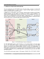


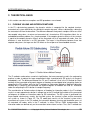
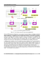
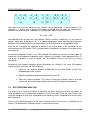

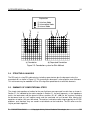


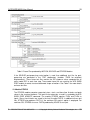


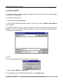
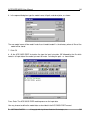

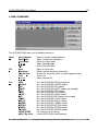
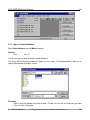

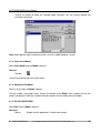
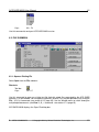
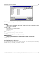
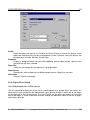
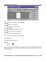
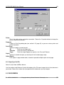
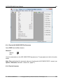


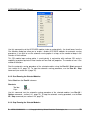
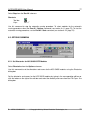
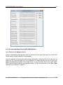
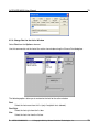
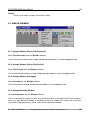
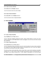
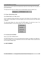


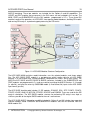
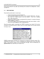
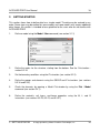
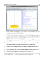

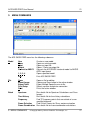
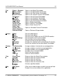

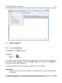
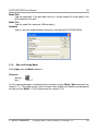
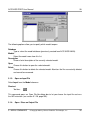

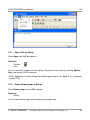

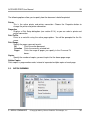


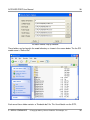
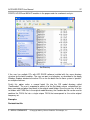


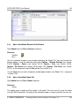

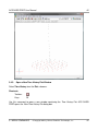
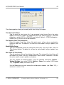
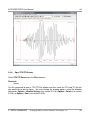
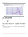
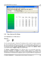
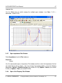
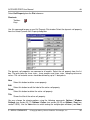
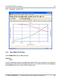
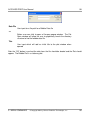
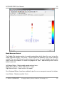
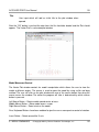
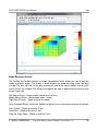


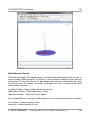

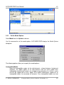
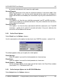
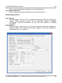


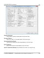


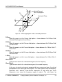


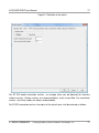


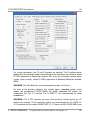


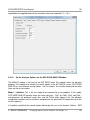

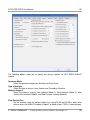

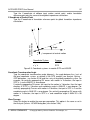


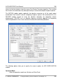


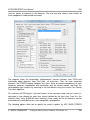


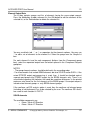
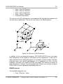
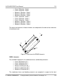
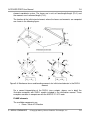
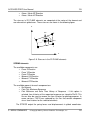


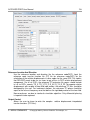

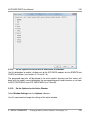
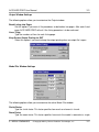
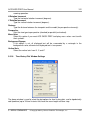
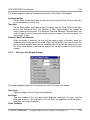

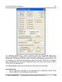

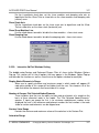
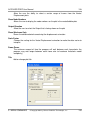

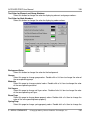
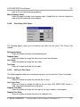
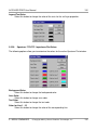
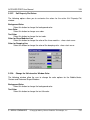
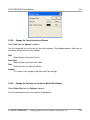
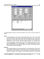

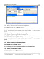

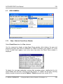
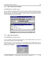

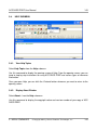
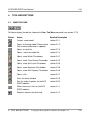


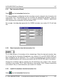

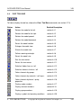


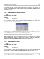


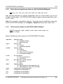


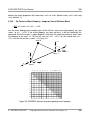

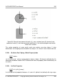


![Validation de modèle dynamique par corrélation cal[...]](http://vs1.manualzilla.com/store/data/006370592_1-78615b94c319ab62d03268ac8d13aa3e-150x150.png)