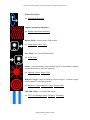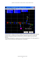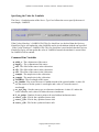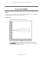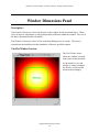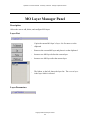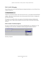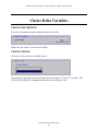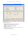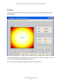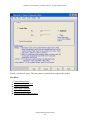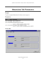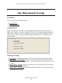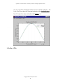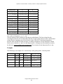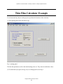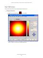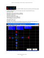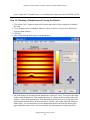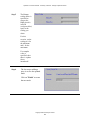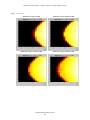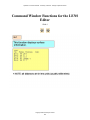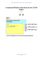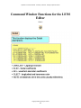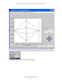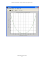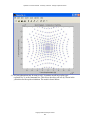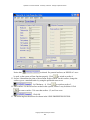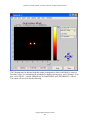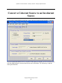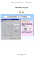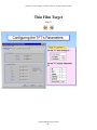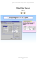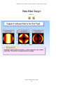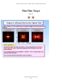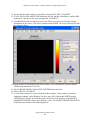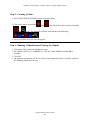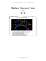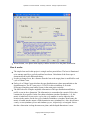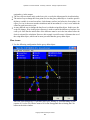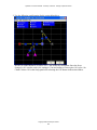
1
OptiScan 7.3.0 User’s Manual
College of Optical Sciences
University of Arizona
OptiScan 6.2.0 User’s Manual - University of Arizona - College of Optical Sciences
Table of Contents
Introduction:
Computer Requirements
Making Optiscan Writable
Introduction to Optiscan
OptiScan Basics (a.k.a., If you don’t read anything else, read this.)
Startup Wizard Panel
An Introduction to the Project Workspace
Main Help Page
Chapter 1: Objects
About Panel
Cheat Sheet
Detector
Multiple Detector Example
Multiple Detector Layers
Fiber Detector
Source Object
Source Type Panel
Beam Splitter Object
Beam Splitter Settings Panel
Lens Object
Lens Editor Panel
Lens Properties Panel
Lens Sampling Panel
Lens Setup Panel
Propagation Options Panel
Lens View Editor
Lens Viewer Settings
Aberrations Panel
Link Parameters Panel
Using Tilts
TILTX
TILTY
TILTZ
Copyright 2005 University of Arizona
1
OptiScan 6.2.0 User’s Manual - University of Arizona - College of Optical Sciences
Targets
Target Window
Multiple Layers
The Layer Manager Panel
Multilayer File Format
Reflective Target
Transmission Target
Thin-film Target
TFT Settings Panel
TFT Layer Manager Panel
Magneto-Optical Target
MO Settings Panel
MO Layer Manager Panel
Multiple Level Lithography
Multilayer Fluorescent Object
Polarization Object
Polarization Settings Panel
Propagation Object
Angular Spectrum Propagation
Chapter 2: Delta Operations
Gooey Delta Panel
Custom Gooey Variable Configuration Panel
Delta Function M-files
Script Tool Properties
Choice Delta Variables
Scalar Delta Variables
String Delta Variables
Layer Specific Gooey Delta Variables
Surface Specific Gooey Delta Variables
Monte Carlo Analysis
RSS Analysis
Chapter 3: Modifying Objects
The "Add A Piece" Wizard
Input From File Panel
Catalog Pattern Panel
Custom Pattern Generator
Custom Pattern Example
Copyright 2005 University of Arizona
2
OptiScan 6.2.0 User’s Manual - University of Arizona - College of Optical Sciences
Dimensions Tab Parameters
One Dimensional Grating
One Dimensional Grating - Rectangular
One Dimensional Grating - Fourier Series - Catalog
One Dimensional Grating - Fourier Series - Direct Input
One Dimensional Grating - Fourier Series - Trapezoid
Bitmap Scaling Panel
Dimensions Panel
Chapter 4: Setting Simulation Parameters
The Model Panel
Sampling
Setup
Chapter 5: Viewing Objects/Results
Basic Viewer
The Zoom Control
Chapter 6: Working with the Command Line
Command Line Functions
Auxiliary Command Line Functions
pupil
fir
sur
field
seidel
rayfan
wavefan
spot_diagram
find_chiefray_intercepts
Chapter 7: Supplemental Calculators
Gaussian Beam Width Calculator
Laser Diode Beam Calculator
Optical Fiber Calculator
RCWT Calculator
Thin Film Calculator
Copyright 2005 University of Arizona
3
OptiScan 6.2.0 User’s Manual - University of Arizona - College of Optical Sciences
Chapter 8: File Operations
Save Filename Panel
Fields Panel
Chapter 9: User Defined Operations
Custom Mathematical Operations (MOP’s)
Chapter 11: Tutorials
Tutorials Main Page
Simulate Scanning a Laser Beam Over a Target
A Simple Disk Tutorial
Scanning Spot Tutorial
Lens Functions
Auxiliary Command Line Functions
Lens Tilts
Creating a Thick Lens
Coherent and Incoherent Point Source Imaging
Convert a Coherent Source to an Incoherent Source
Incoherent Lens Settings
TFT
Fresnel Diffraction
Multilayer Fluorescent Target
Chapter 12: Sample Projects
GS Beam Shaper
Reference
Troubleshooting and FAQs
User Notes
Index
Copyright 2005 University of Arizona
4
OptiScan 6.2.0 User’s Manual - University of Arizona - College of Optical Sciences
Computer Requirements
Optiscan requires the following software:
MATLAB 6.5.2
Internet Explorer 5.0
Zemax Lens Editor. (for importing lens files only)
Optiscan requires the following hardware:
At Least 512 MB of RAM
At Least a 1 GHz Processor.
100 MB of disk space (500 MB recommended for data storage)
Copyright 2005 University of Arizona
5
OptiScan 6.2.0 User’s Manual - University of Arizona - College of Optical Sciences
Making Optiscan Writable
Windows 98
1.
2.
3.
4.
5.
Click "Start", choose "Find", then choose "Files or folders"
Click Browse and choose your main Optiscan directory
In the box labeled "Named" type "*.m"
Click "Find Now"
When your computer finishes searching, select all the files that were found by clicking on
the first file and then hold the "Shift" key down on your keyboard while clicking on the last
file
6. Right click on the selected files
7. Choose properties and uncheck the "Read-only" option and click OK
8. Repeat steps 3-7 using "*.mat" in step 3
Windows 2000
1.
2.
3.
4.
Right click on your main Optiscan directory and choose properties.
Uncheck the "Read-only" option and click apply
Choose "Apply changes to this folder, subfolders, and files" and click OK
Click OK on the properties window
Copyright 2005 University of Arizona
6
OptiScan 6.2.0 User’s Manual - University of Arizona - College of Optical Sciences
Introduction
The OptisScan program is a tool for simulating the operation of optical systems. What
differentiates OptisScan from other simulation software is the wide range of wave-optics
phenomena that are available and the graphical user interface (GUI). OptisScan can be used as a
simple demonstrator of idealized systems, or the user can simulate complicated effects like
interaction with multiple-layer targets and vector diffraction.
OptisScan operates in the MATLAB environment, and all of the commands available to
MATLAB users are also available to OptisScan users.
The motivation for developing the OptisScan program came from an interest in efficient use of
student time. Over the last sixteen years, our research group has developed many very powerful
simulation codes for various applications, like optical data storage and laser scanning. Each time
a new student joins our group, it takes a significant amount of time to learn the codes. An average
learning curve was about six months. I wanted to design an easy-to-use graphical user interface
that would connect the different codes in order to shorten the learning curve. Although it took
over a year to get OptisScan to a useable state, the results are worth it. In one case a student
started with no knowledge of the program and was producing results in less than one hour. At this
point, not all of the features are operational, but we are working on it. We will continue to
develop the program and provide new features as time marches on. I hope that you have as much
fun using OptisScan as I have had writing it.
Tom Milster
Copyright 2005 University of Arizona
7
OptiScan 6.2.0 User’s Manual - University of Arizona - College of Optical Sciences
OptiScan Basics
(a.k.a., If you don’t read anything else, read
this.)
OptiScan works by segmenting various portions of optical simulation problems into objects. For
example, a laser source can be described by object 1. The laser source emits a light beam that
interacts with object 2, a lens system. The lens system directs the laser energy onto a target plane.
The energy in the target plane can be saved to a file with object 3, which is a utility object that
doesn’t affect the optical field distribution.
In general, the interaction with each object can be pictured as shown in the figure below.
The working matrices of the calculations are Ext, Eyt, Ezt, Exr, Eyr and Ezr. These six
two-dimensional matrices describe the polarized electric field complex amplitude of a
’transmitted field’ and a ’reflected field’. The coordinate system for all matrices is described by
the sysxvec and sysyvec vectors, which define the spatial positions of the columns and rows,
respectively, of the field matrices.
The OptiScan object can modify any of the field matrices, depending on its function. For
example, a transmission target will affect the transmitted fields, and a reflective target will affect
the reflected fields. In each case, the corresponding coordinate system vectors are appropriately
modified. An optics object transforms the field distribution in the object plane with object-plane
Copyright 2005 University of Arizona
8
OptiScan 6.2.0 User’s Manual - University of Arizona - College of Optical Sciences
coordinates, propagates the laser beam through the lens system, and provides the transmitted field
distribution in the image plane with the proper image-plane coordinates. A beam splitter object
will modify both the reflected and transmitted fields.
A partial list of available OptiScan objects includes:
Optics (lens system)
Reflective target
Transmission target
Multiple-layer fluorescent target
Thin-film target
Magneto-optic target
Simple responsivity detector
Fiber detector
Source
Propagate
Beam splitter
Polarization element
Tools:
Look (utility object)
Gooey delta (utility object)
Script delta (utility object)
Save fields (utility object)
Restore fields (utility object)
Mathematical operation
Usually, calculations require more than one object. For example, a laser source is often combined
with a lens to make a field distribution at the target plane, which can then be saved to a file.
Therefore, objects must be ’linked’ together to form a calculation ’chain’. With the graphical user
interface of OptiScan, ’building’ the chain takes the form of making ’links’ (arrows) between
objects. Before a calculation, the user specifies the order of the links in the chain that will be
used. An example chain is shown below for the source-lens-save calculation. Notice that the links
are shown as yellow arrows. The first link between the source and the lens is assigned ’T:1’,
which indicates that it is the first link in the chain calculation and it works on the transmitted
fields from the source. The second link is assigned ’T:2’, so the save object will take the
transmitted fields calculated from the lens and save them in a file. The mechanics of building the
objects, assigning links and specifying the order of calculation in the chain are provided in this
user’s manual. In addition, properties of an object can be edited by selecting the object with the
mouse button and then selecting the ’edit’ option. A new window opens that contains information
that can be modified.
Copyright 2005 University of Arizona
9
OptiScan 6.2.0 User’s Manual - University of Arizona - College of Optical Sciences
Many analysis problems require that some aspect of the system must be modified between
calculations. In OptiScan, one powerful way to adjust an object’s parameters is with the gooey
delta object. For example, if the user desires analysis of the electric field distribution in the target
plane as a function of the distance from the last surface of the lens, a gooey delta object can be
linked to the lens, as shown below.
If the gooey delta object is the first link in the chain, it will change the appropriate surface
thickness before the source- lens-save calculation takes place. Multiple source-lens-save
calculations can be implemented automatically by setting the ’Chain Count’ variable to a value
greater than 1. (The Chain Count variable is shown in an edit window after the ’Calc’ button in
the lower right-hand corner of the project window is selected.) The gooey delta object will then
set the appropriate thickness before each of the chain calculations. Notice that the gooey delta’s
link to the lens object is assigned ’O:1’, which indicates an ’object/field operation’ link that does
not change the values of the field matrices.
In developing the OptiScan program with students, it became clear that many simulation
problems require additional processing of the optical fields beyond what is available with the
standard objects. Therefore, the Mathematical Operation (MOP) object was created, which allows
the user to operate on the Ext, Eyt, Ezt, Exr, Eyr and Ezr field matrices and the sysxvec and
sysyvec coordinate vectors. For example, assume that the nonlinear response of a material is
desired as a function of lens defocus. A MOP object can be added to the chain in order to perform
the nonlinear calculation, as shown below.
Copyright 2005 University of Arizona
10
OptiScan 6.2.0 User’s Manual - University of Arizona - College of Optical Sciences
The user calculation is written as a simple Matlab function. The user accesses field matrices
inside the function through the ’simdata’ structure. For example, if the user wants to access the
Ext field, the command MyExt = simdata.Ext can be used. If the fourth-order response is
calculated, the simple series of commands:
MyExt4 = abs(MyExt).^4;
simdata.Ext = MyExt4;
assigns the fourth-order field distribution to the Ext working matrix. Other field matrices and
system information can be accessed through the simdata structure.
A large amount of effort went into making sure that, during setup of the objects in your project
and during the calculation, the ’loading’ of variables in the Matlab command-line interface
window is minimized. That is, OptiScan is virtually transparent to the command line. The user is
free to use any of the powerful Matlab functions in the workspace without interfering with
OptiScan. An exception occurs with plotting. If the user wants to plot data using any of the
Matlab plotting routines from the command line, a new figure window should be opened first. If
not, some of the graphical user interface objects in the OptiScan project window may be
overwritten. For example, if the user wants to graph yvec versus xvec, the command line should
take the following form: figure; plot(xvec,yvec).
One common problem with users is that they loose track of how much data they are generating.
The ’save fields’ object is very useful, but, in multiple calculations with large Chain Count, the
amount of data can easily be in the GB range or more. A little forethought, housekeeping and
planning go a long way. For example, if only a scalar calculation is required, Ext is the only field
matrix that requires a non-zero value.
In addition to OptiScan objects, several useful calculators are available that do not require a chain
calculation. A partial list of these calculators, which are accessible through the ’Accessories’
menu item in the project widow, includes:
Optical fiber beam calculator
Gaussian beam width calculator
Laser diode beam calculator
Thin film calculator
RCWT calculator (rigorous coupled-wave theory)
Glass dispersion calculator
Calculations in OptiScan are organized into ’projects’. That is, each new type of calculation
should be given its own project and saved separately. For example, the calculation shown in the
previous figures might be assigned the name ’nonlinear_defocus’ and saved under that name by
selecting ’save project as’ under the ’System’ menu item in the project widow. The name of the
new project can also be specified when a new project is opened. It is a good idea to ’save project’
periodically during the construction of a new project, in order to avoid potential problems with
computer crashes. Existing projects can be opened by selecting ’Open Existing OptiScan Project’
Copyright 2005 University of Arizona
11
OptiScan 6.2.0 User’s Manual - University of Arizona - College of Optical Sciences
on the entry widow at any time after startup.
OK, you are probably anxious to get started. Hopefully, you have at least read these ’OptiScan
Basics’ pages. You really should go through the rest of the manual, but, if you are like me, you
probably won’t access the ’Help’ button until after your first blunder or two. I strongly suggest
that you now go through several tutorials and then play around with the sample projects before
building your own project. In any case, I hope you enjoy the program.
On a final note, please understand that OptiScan is a ’Work in Progress’, and it is being made
available at a very reasonable fee. The primary purpose for the program is research. License fees
are used to support further development of the program and student education. We welcome your
comments and suggestions, and bugs will be promptly displayed on the OptiScan web site.
Licensed users will receive updated code as it becomes available.
Copyright 2005 University of Arizona
12
OptiScan 6.2.0 User’s Manual - University of Arizona - College of Optical Sciences
Startup Panel
Description :
The Startup Panel allows the user to choose whether he/she wants to open an existing Optiscan
Project or create a new Optiscan Project.
When a new Optiscan Project is created, a new folder/directory is created to put it in. The
Optiscan Project File typically has the same name as the folder that it is stored in. This file is
commonly called the Optiscan Project since it is the file that is opened when the Open Existing
Optiscan Project option is chosen.
Copyright 2005 University of Arizona
13
OptiScan 6.2.0 User’s Manual - University of Arizona - College of Optical Sciences
How to Use :
(1) The first option to take a look at is Open New Optiscan Project. This option allows you to
start a project in an empty workspace but also gives the opportunity to name the project whatever
you choose. Below is a screenshot of how the user can name the project as well as the folder it is
stored in.
The user is free to name the Project Name something entirely different from the Project Folder
but it is a generally good rule to have the folder the same as the Project Name. This means to
keep each different project in its very own folder. After the names have been chosen, click OK to
open up a new workspace with the project names specified. If a small box pops up asking if you
want to Overwrite Existing Project File?, this means that there is already a project with that
name. Either click Yes to overwrite or No to rename it to something else.
Copyright 2005 University of Arizona
14
OptiScan 6.2.0 User’s Manual - University of Arizona - College of Optical Sciences
(2) The second option is to instead choose to Open Existing Optiscan Project. A completely
different Project Manager window will show up.
Copyright 2005 University of Arizona
15
OptiScan 6.2.0 User’s Manual - University of Arizona - College of Optical Sciences
This Project Manager has a few neat features. First it will show the last project file that was saved
in the form of "project_name".mat. If this is the project desired to be open, click OK and
OptiScan will load it up. If another previously saved project is desired click on the upper tab
section labeled Browse. The correct directory can be found and the corresponding project. Likely
the project .mat file will be located in a folder of the same name. While browsing, at the bottom
of this window is a little section that displays all project files that are stored in the selected folder
and allows quick access to choose the desired folder. Likely only one project file will be stored in
the folder though.
Tips on saving projects
Even though you can name a brand new project what you want from startup, the best way is to
just open a the generic myproject.mat and when it’s time to save choose Save Project As from the
file menu.
It will prompt to name the file and in which folder. The browser window should open to the
default proj folder which is where the saved project will remain. What this will do is create a new
folder with the project name and the project stored inside. Both the folder and the .mat file will
have the same name keeping things very convenient. Another way to save the project is to just
choose Save Project from the file menu. This will just save the current project under the same
name effectively replacing it with a new copy. If a name was never specified then it is just saving
the current project as myproject.mat.
Copyright 2005 University of Arizona
16
OptiScan 6.2.0 User’s Manual - University of Arizona - College of Optical Sciences
Project Workspace
Description:
The Project Workspace is the main window of Optiscan.
Important Demo
Main Project Workspace
System Menu
Build Menu
Accessories Menu
Object Controls
Links
Help Button
Calc Button
See Also
Important Demo
To learn about the workspace, it is recommended that new users have fun with the Simple Disk
Tutorial. This tutorial uses the concepts which are discussed below.
Main Project Workspace
This document describes the various features of the Main Project Workspace:
Copyright 2005 University of Arizona
17
OptiScan 6.2.0 User’s Manual - University of Arizona - College of Optical Sciences
The name of the OPTISCAN system, in this case simpledisk.mat, is placed in the window’s
titlebar.
System Menu
Save
Allows the user to "save" the current system to disk. Many
of the OPTISCAN model’s data are stored in separate files.
These are saved immediately. For example, if the source’s
electric fields are modified using the "Add A Piece" wizard,
then they are immediately saved. The source’s dimensions
are not saved until the system is saved.
Save As
Allows the user to save the current system to a new a project.
The entire project is copied to the new project folder.
Preferences
Allows the user to set global sampling parameters and other
values.
Close
Closes the current system. The user is asked if the current
system should be saved before the Project Window is closed.
Build Menu
The "Build Menu" allows the user to create physical optics objects. If
the "Source" item was chosen from the "Build menu," then
OPTISCAN creates a new source and places it in the
upper-righthand-corner of the project workspace:
The various items that can be created are described in the Optiscan
Cheatsheet
Accessories Menu
Copyright 2005 University of Arizona
18
OptiScan 6.2.0 User’s Manual - University of Arizona - College of Optical Sciences
Optical Fiber Calculator
Gaussian Beam Width Calculator
Laser Diode Beam Calculator
Thin Film Calculator
RCWT Calculator
Glass Dispersion Calculator (help page coming
soon)
Object Controls
When "Arrange Object" is actived (clicked on), then objects may be
relocated in the project workspace by dragging them around with the
mouse.
When "Edit Object" is actived (clicked on), the objects in the project
workspace may be editted by clicking on them.
When "Delete Object" is activated (clicked on), the objects in the
project workspace may be deleted by clicking on them.
It may be more convienient to right click an object in the project
workspace and then choose the desired action from the menu which is
displayed:
Links
Copyright 2005 University of Arizona
19
OptiScan 6.2.0 User’s Manual - University of Arizona - College of Optical Sciences
Links are used to specify how electric fields propagate through an
OPTISCAN model. See the Links page for more information. The
following model shows the electric fields propgating from a source to
a reflective target to a plot:
When "Make Link" is activated (clicked on), links can be created by
clicking on the object, which is the source on the electric field, and
then clicking on the object which the electric field is being propagated
to.
When "Edit Link" is activated (clicked on), the properties of a link
can be displayed for modification by clicking on it. The following
image shows what happens when a link’s type is changed:
When "Delete Link" is activated (clicked on), the links in the project
workspace can be deleted by clicking on them.
An OPTISCAN link shows how an electric field propagates from one
optics object to the next. A chain specifies the order in which the links
are evalulated. In the following system:
The link labeled "0:1" is evaluted first, the link labeled "T:2" is
evaluated second, and the link labeled "R:3" is evaluated last.
Copyright 2005 University of Arizona
20
OptiScan 6.2.0 User’s Manual - University of Arizona - College of Optical Sciences
Help Button
- brings up a Web Browser to display the OPTISCAN Help Desk.
Calc Button
- initiates a simulation by displaying the System Preferences Dialog.
See Also
Simple Disk Tutorial
Links
Copyright 2005 University of Arizona
21
OptiScan 6.2.0 User’s Manual - University of Arizona - College of Optical Sciences
OPTISCAN Help Desk
Introduction
An Introduction to Optiscan
OptiScan Basics
A Simple Disk Tutorial
Startup Wizard Panel
An Introduction to the Project Workspace
The About Panel
Reference
Troubleshooting and FAQs
User Notes
Update Descriptions
Computer Requirements
Optiscan Tutorials
Optiscan Cheat Sheet
Table of Contents (by subject)
Index (in alpahbetical order)
Publications
Email Comments and Suggestions to:
[email protected]
Milster Group Home Page
Copyright 2005 University of Arizona
22
OptiScan 6.2.0 User’s Manual - University of Arizona - College of Optical Sciences
New features in OPTISCAN version 6.1
1. Compatability with MATLAB 6.5.
2. Detector Layer Option:
Located in the Detector Properties Editor. A new feature added to the Simple Responsivity
Detector that allows the user to have multiple layers inside one detector object.
3. Fiber Detector:
Located in the build menu of the project workspace. Calculates the coupling efficiency of an
optical fiber.
4. Optical Fiber Calculator:
Located in the accessories menu of the project workspace. Calculates the 1/e 2 radius of the
|E| 2 Gaussian propagation mode in a single mode fiber.
5. TFT Calculator:
Located in the accessories menu of the project workspace. Calculates the transmission and
reflectivity of a multi-layer thin film structure.
6. Waveguide Analyzer:
Located in the accessories menu of the project workspace. The OSC Wave program that
functionally evaluates a waveguide. It provides the eigenfunctions and eigenvalues of the
scalar wave equation for the principle component of the electric field of all bound modes.
7. Time Stamp:
A time stamp is now included in detector output files.
8. Added Examples to Help Pages:
Custom Pattern Generator
Optical Fiber Calculator
Laser Diode Calculator
Gaussian Beamwidth Calculator
TFT Calculator
9. PDF version of the user’s guide now available.
10. Because the diffraction calculation is done with sampling of the numerical aperture both in
image space and object space, this will cause the XY coordinates in diffraction simulation
results to not match the first order expectation. At low NA, the mismatch is quite small;
however, we have to correct the difference between SIN (Numerical Aperture) and TAN
(First Order).
Copyright 2005 University of Arizona
23
OptiScan 6.2.0 User’s Manual - University of Arizona - College of Optical Sciences
New features in OPTISCAN version 6.0
1. Compatibility with Matlab v6.0 and v6.1
2. Improvements to the GUI Delta object:
The GUI Delta object can now be used to change lens parameters.
Layer specific variables for the MO and TFT objects can now be changed (previously
only the overall variables could be changed).
Monte-Carlo analysis can now be done using the GUI Delta. Both uniformly distributed
random numbers and gaussian distributed random numbers can be generated.
RSS analysis is now available, and we have a highly experimental version of the auto
range option.
3. XFDTD Conversion Calculators:
These Calculators are used to interface time-domain output of the XFDTD finite difference time domain program from Remcom, Inc., to Optiscan. XFDTD produces files that contain
snapshots of the electric field from near-field geometries. The calculator converts XFDTD
time-domain data into complex amplitude and phase for x, y, and z polarization directions.
Complex data are in Matlab matrix format. Please see the help files for more information.
4. Improvements to the 2D viewer:
A new option is added that allows the user to save the current layer to a new file for use
in another object.
A menu of several color maps is available so the user can easily switch between
different views of the same data. The available color maps are: jet, hot, gray, and hsv.
Other color maps and figure operations can be entered via the Matlab command line.
5. Laser diode calculator:
The Laser Diode Calculator is a shortcut to calculate field distributions for known laser
diodes. One of the main uses of this calculator is to lookup or calculate values to use in the
custom pattern generator. Most laser diode specifications list far field divergence in degrees,
while Optiscan works with the spot size in meters.
6. Transmission target:
A new target is available that operates on an incident two-dimensional field with a matrix
representing complex index of refraction and depth information. See the help pages for more
information.
7. Various improvements are made to the optics module that allow better accuracy for high-NA
systems and micro-optical systems.
8. Propagation object (angular spectrum propagation):
Upgraded to work with negative distances.
The interface panel is updated to be more user friendly.
Now works with incoherent sources.
9. Improved descriptions of the reflection target and the new transmission target are available
in the help pages.
Copyright 2005 University of Arizona
24
OptiScan 6.2.0 User’s Manual - University of Arizona - College of Optical Sciences
10. Version 10 Zemax files can now be used with OPTISCAN. If OPTISCAN encounters part of
the lens description that it can’t decode, that part of the lens description is printed in the
command-line window.
11. Axis menu in the Lensview panel:
Axis settings, such as ’normal’ and ’equal’ can be entered via the menu bar
12. User Notes Page:
A new help page accessible from the Main help desk that lists miscellaneous notes for users.
13. Detector help page:
Help documentation is now available for the detector object.
14. The ’fir’ (first-order optics) command-line program in OPTISCAN now is activated by
typing ’optfir’. Please see the help pages for more detailed instruction on using command-line
inputs in OPTISCAN.
Copyright 2005 University of Arizona
25
OptiScan 6.2.0 User’s Manual - University of Arizona - College of Optical Sciences
Publications
A user friendly diffraction modeling program, in Conference Digest of Optical Data Storage
Topical Meeting, p. 60, IEEE, New York (1997)
An Optical System Simulation Model in MATLAB Rose Early, Tom D. Milster Oral
presentation SW04-415 at Opto-Southwest 2001
Physical Optics Simulation in Matlab for High-Performance Systems Tom D. Milster
OPTICAL REVIEW Vol. 10, No.4 (2003) 246-250
Copyright 2005 University of Arizona
26
OptiScan 6.2.0 User’s Manual - University of Arizona - College of Optical Sciences
An Optical System Simulation Model in
MATLAB
Rose Early, Tom D. Milster (Optical Sciences Ctr./University of Arizona, Tucson, AZ 85721)
Motivation
The motivation for developing the OPTISCAN program came from a need for a flexible
physical-optics simulator that could deal with specialized problems including scanning for optical
data storage, laser-to-fiber coupling, lithography, and near-field microscopy. The program also
needed to have the ability to perform specialized operations including: vector high-NA focusing
and import/export for XFDTD and Zemax files The other main motivation was an interest in
efficient use of student time. Over the last ten years, our research group has developed many very
powerful simulation codes for various applications, like optical data storage and laser scanning.
Each time a new student joined our group, it took a significant amount of time to learn the codes.
An average learning curve was about six months. We wanted to design a program that would
connect the different codes in order to shorten the learning curve. Although it took over a year to
get OPTISCAN to a useable state, the results are worth it. In one case a student started with no
knowledge of the program and was producing results in less than one hour. Now new students
can use the results of previous students efforts to provide consistent scientific output.
Design Philosophy
Optiscan was designed as a research tool. Its a Non-commercial program, but is available through
the University of Arizona. OPTISCAN is flexible so that custom Matlab program modules for
specific applications can be easily incorporated into calculations. It was designed to have an
easy-to-use Graphical user interface. Optiscan came directly from our research efforts, nothing
was "canned." Optiscan was written in Matlab because Matlab already has many useful
commands that can be used in Optiscan for optical calculations, and is set up for general
mathematical and scientific applications.
System Requirements
Software:
MATLAB 5.3.1
Internet Explorer 5.0
Hardware:
Copyright 2005 University of Arizona
27
OptiScan 6.2.0 User’s Manual - University of Arizona - College of Optical Sciences
At Least 64 megabytes of RAM
At Least a 200 MHz Processor.
60 MB of disk space (500 MB recommended for data storage)
Workspace
This is an example of the Workspace:
The workspace is the basic user interface for Optiscan. Although the Matlab command line is
available to the user, most of the actions required to perform calculations are performed through
the workspace GUI.The workspace consists of objects that are connected by links. The direction
of the arrow in each link shows the flow of information and can be thought of as the direction of
the flow of light in the system. Objects represent physical elements in the optical system like laser
sources, lenses, targets, and detectors. Objects can also represent more programmatic operations,
like saving or retrieving data. The links are placed in a "chain" that is evaluated sequentially. The
flexibility of choosing different combinations of links in chains allows the user to run slightly
different simulations without making a whole new project. The overhead for the Optiscan
workspace is very low. The user has the full utility of Matlab available in the command line
Copyright 2005 University of Arizona
28
OptiScan 6.2.0 User’s Manual - University of Arizona - College of Optical Sciences
interface with only three variables dedicated to the operation of Optiscan.
Direct Physical Representation
Beam Splitter - splits electric fields into a transmitted part and a reflected part.
Detector - allows the user to specify an arbitrary detector using a BMP detector
mask or any of the custom or catalog patterns.
Multilayer Fluorescent Target
Photo-resist based multiple layer lithographic target where the exposure and
development in the resist is calculated
Optical Lens - the lens group can be created in Zemax or specified directly by the user. It
allows the user to select the type of propagation formulas which are used to calculate the
propagation of the electric fields through the lens group. Propagation can be either scalar or
vector.
Source - create and manage source fields. Coherent and incoherent source types
are supported Any of the custom or catalog patterns can be used.
Copyright 2005 University of Arizona
29
OptiScan 6.2.0 User’s Manual - University of Arizona - College of Optical Sciences
Reflective Target - can be built using bitmap masks or any of the custom or
catalog patterns.
Thin Film Target - vector interaction of focused field with a homogeneously
layered object
Magneto-Optical Target - same as thin film target with the addition of one
magneto- optic layer.
Special Simulation Tools
Delta Object - allows the user to modify the parameters of other components
during simulation
Look Object - allows the user to look at results graphically during a simulation
run.
Mathematical Operation - perform custom calculations on the system’s electric
Copyright 2005 University of Arizona
30
OptiScan 6.2.0 User’s Manual - University of Arizona - College of Optical Sciences
fields. Input as a Matlab m-file.
Angular Spectrum propagation -
Save Fields - save electric fields to disk.
Restore Fields - restore electric fields from a disk
Detail of Optics Module
Copyright 2005 University of Arizona
31
OptiScan 6.2.0 User’s Manual - University of Arizona - College of Optical Sciences
The Optics Module uses direction cosine propagation. It offers direct conversion of Zemax files.
It has a flexible aberration calculation; the user can choose from Ray-based, Zernike, or
User-input. The calculation has the ability to do tilts, decenters and aspheres. The diffraction code
includes Huygens, high numerical aperture and out-of-focus plane calculations. There are Critical
and Köhler illumination options. The module offers User-selectable pupil sampling.
Physical Optics Fields
Optiscan uses matrices to describe the amplitude and phase of vector electromagnetic fields at
each node in the calculation chain. Both transmitted and reflected field information is available to
the user
Copyright 2005 University of Arizona
32
OptiScan 6.2.0 User’s Manual - University of Arizona - College of Optical Sciences
2D - Viewer
The 2d-viewer helps maintain consistency by providing a single interface across several objects,
namely the Sources, Targets, and Detectors. The 2d-viewer is where custom and catalog patterns
come in.
Catalog Patterns
These are the pre-made patterns that are available in Optiscan:
Uniform
Data Mark
Circle
High Frequency data pattern
Low Frequency
Inter-symbol interference data pattern
Custom Patterns
These are the patterns that can be created to the users specification:
Gaussian
Super Gaussian
Hermite
Mix - and - match
Exponential
Gaussian
SuperGaussian
Linear Ramp
Pyramid Function
One Dimensional Grating
Copyright 2005 University of Arizona
33
OptiScan 6.2.0 User’s Manual - University of Arizona - College of Optical Sciences
Rectangular
Fourier Series
Work in progress
A new version of Optiscan is scheduled to be released later this Fall.
New features will include:
Monte Carlo Analysis
RSS Analysis
Holographic optical element
Gradient index (Grin) lens surface
Interface with Remcoms XFDTD
Summary
In summary, Optiscan is a flexible, easy-to-use program that was built on previous codes and is
constantly expanding.
Copyright 2005 University of Arizona
34
OptiScan 6.2.0 User’s Manual - University of Arizona - College of Optical Sciences
Chapter 1: Objects
Objects
Objects are the basic functions of Optiscan. They are optical elements that Optiscan is capable of
using. They appear as small icons on the workspace and can be linked together to form an optical
system. The cheat sheet displays all the objects available to Optiscan.
About Panel
Cheat Sheet
Detector
Multiple Detector Example
Multiple Detector Layers
Fiber Detector
Source Object
Source Type Panel
Beam Splitter Object
Beam Splitter Settings Panel
Lens Object
Lens Editor Panel
Lens Properties Panel
Lens Sampling Panel
Lens Setup Panel
Propagation Options Panel
Lens View Editor
Lens Viewer Settings
Aberrations Panel
Illuminator Lens Panel
Link Parameters Panel
Using Tilts
TILTX
TILTY
TILTZ
Targets
Target Window
Multiple Layers
The Layer Manager Panel
Multilayer File Format
Copyright 2005 University of Arizona
35
OptiScan 6.2.0 User’s Manual - University of Arizona - College of Optical Sciences
Reflective Target
Transmission Target
Thin-film Target
TFT Settings Panel
TFT Layer Manager Panel
Magneto-Optical Target
MO Settings Panel
MO Layer Manager Panel
Multiple Level Lithography
Multilayer Fluorescent Object
Polarization Object
Polarization Settings Panel
Propagation Object
Angular Spectrum Propagation
Copyright 2005 University of Arizona
36
OptiScan 6.2.0 User’s Manual - University of Arizona - College of Optical Sciences
Illuminator Lens Panel
Description :
This option is chosen when the lens group describes either Kohler or Critical illumination on a
target. This option must be used with a second lens group that describes the projection camera.
The Illuminator Lens is used with Incoherent Source files.
Illuminator Type :
None
-
No Illuminator Lens is used (default). The sigma is ignored.
Kohler
-
This option assumes that the target (i.e., a lithographic mask) is
placed in the exit pupil of the optical system. The source
distribution is imaged into the entrance pupil of the projection
camera. The incoherent source distribution is resized based on the
entrance pupil diameter of the associated projection camera. The
width of the source is resized so that its image fits within the
projection camera entrance pupil. Changing sigma effectively
apertures the source with an iris. sigma = (diameter of source
image)/(entrance pupil diameter).
Critical
-
This option is not available with the current release.
Copyright 2005 University of Arizona
37
OptiScan 6.2.0 User’s Manual - University of Arizona - College of Optical Sciences
The Projection/Illuminator Lens Portion :
The Projection Lens is the lens that images the illuminated mask target onto the final
target.
Copyright 2005 University of Arizona
38
OptiScan 6.2.0 User’s Manual - University of Arizona - College of Optical Sciences
About Panel
Description :
Each object uses About Panel to allow the user to view important information about that object
quickly. This information includes the name and the description of an object and when the
Optiscan Simulation Engine is allowed to call that object’s calculation procedure. The About
Panel can be viewed with the Right Mouse Button and by displaying an object’s properties.
Displaying the About Panel with the Right Mouse Button :
You can access the About Panel by clicking the Right Mouse Button over an object:
This will display a non-editable version of the About Panel:
Copyright 2005 University of Arizona
39
OptiScan 6.2.0 User’s Manual - University of Arizona - College of Optical Sciences
The Editable Version of the About Panel:
The editable version of the About Panel is displayed by editing an object’s properties. Use the
Edit Object feature and then click on the object you wish to edit:
The About Panel can be viewed by displaying the About Tab:
Some object editors require the user to select "Properties" from the "Go" menu and then click the
"Go" button to actually view the object’s properties.
Specifying an Object’s Name and Description :
The About Panel allows the user to enter a friendly name and a useful description about the
object.
Name The Name field is used to give a user friendly name to an object. The Optiscan
Simulation Engine uses this name when it prints out its messages. The Optiscan
Modeling Environment uses it to label windows.
Desc
The Desc field can be used to enter object important information such as a specific
notation.
Copyright 2005 University of Arizona
40
OptiScan 6.2.0 User’s Manual - University of Arizona - College of Optical Sciences
Specifying an Object’s Name and Description :
The "Calculate" portion of the About Panel allows the user to specify when an object’s calculation procedure is invoked:
Every Chain Calculation
Specifies that the associated object should have its calculation procedure called everytime that
the Opitiscan Simulation Engine determines that that object should be calculated..
First Chain Calculation
Specifies that the the associated object’s calculation procedure should only be called during
the first chain calculation.
Based On Flag Vector
Specifies that the the associated object’s calculation procedure should be called based on the
Flag Vector:
Given this Flag Vector, the Optiscan Simulation Engine would be able to call the associated
object’s calculation procedure during the first, third, fifth,... chain calculations.
Last Chain Calculation
Specifies that the the associated object’s calculation procedure should only be called during
the last chain calculation.
Based On Input Link
Specifies that the object’s calculation procedure should be called based on the calculation
setting of the previous link.
If a link uses this setting, the Optiscan Simulation Engine will present the user with an Error
Dialog Message.
Copyright 2005 University of Arizona
41
OptiScan 6.2.0 User’s Manual - University of Arizona - College of Optical Sciences
Optiscan Cheat Sheet
Beam Splitter - splits electric fields into a transmitted part and a reflected
part.
see: Beam Splitter Settings
Delta Object - allows the user to modify the parameters of their model
components during simulation.
see: Modifying Parameters Easily; Script Tool (Advanced!)
Detector - allows the user to specify an arbitrary detector using a 256 color
BMP detector mask.
see: Optiscan Viewer; Scanning Demo
Look Object - allows the user to look at results graphically during a
simulation run.
see: Optiscan Viewer
Mathematical Operation - perform custom calculations on the system’s
electric fields.
see: Configurable Variables (Easy Editing of Custom Script Variables);
Script Tool (Custom Scripts)
Optical Lens - load a lens group created in zemax. allows the user to select
the type of propagation formulas which are used to calculate the propagation
of the electric fields through the lens group.
see: Lens Viewer; Lens Editor; Propagation Methods; Lens Settings;
Copyright 2005 University of Arizona
42
OptiScan 6.2.0 User’s Manual - University of Arizona - College of Optical Sciences
Polarization Object
see: Polarization Properties;
Angular Spectrum propagation
see: Angular Spetctrum Parameters;
Restore Fields - restore electric fields to disk.
see: Fields Panel, Source Type
Save Fields - save electric fields to disk.
see: Fields Panel
Source - create and manage source fields using 256 color bitmaps. coherent
and incoherent source types are supported.
see: Optiscan Viewer, Source Type
Reflective Target - create and manage reflective targets. a reflective target
is built using 256 color bitmap masks.
see: Reflective Target Optiscan Viewer, Window Panel
Thin Film Target - create thin film targets.
see: TFT Layer Manager Panel; Tft Demo; Tft Settings
Copyright 2005 University of Arizona
43
OptiScan 6.2.0 User’s Manual - University of Arizona - College of Optical Sciences
Transmission Target - create and manage transmission targets. a
transmission target is built using 256 color bitmap masks.
see: Transmission Target Optiscan Viewer, Window Panel
Magneto-Optical Target - create magneto-optical targets
see: MO Layer Manager Panel; MO Settings
Multilayer Fluorescent Target - create multilayer fluorescent targets.
see: Multilayer Fluorescent Target; MLF Demo;
Copyright 2005 University of Arizona
44
OptiScan 6.2.0 User’s Manual - University of Arizona - College of Optical Sciences
Simple Responsivity Detector
Description:
The detector object allows the user to simulate an integrating detector in an optical system. That
is, the detector integrates the optical irradiance over the exposed surface of the detector and saves
the integrated result as a single value in units of Amps.
Getting Started
Editing the Detector
Using the Detector
Multiple Detector Example
Adding Layers to a Detector
Command Line Variables
Notes
See Also
Getting Started:
Click Build -> Detectors -> Simple Responsivity in the main model panel.
Click on Arrange Object and drag the detector icon
to the desired position.
Editing the Detector:
The default detector in Optiscan is square shaped with dimensions of (1mm x 1mm) and a
sampled array size of (500x500). This detector has a responsivity such that only the upper right
hand corner of the total detector area is sensitive to the light impinging on the detector. Note that
the data values given in the 2-D array represent the detector responsivity and have units of
AMPS/WATT.
Copyright 2005 University of Arizona
45
OptiScan 6.2.0 User’s Manual - University of Arizona - College of Optical Sciences
The size and sampling of the detector can be reconfigured by the user by selecting the
PROPERTIES menu item and clicking on GO. This opens the DETECTOR DIMENSIONS
window. This window functions exactly like the DIMENSIONS windows for the SOURCE
object and the many TARGET objects. The size, offset and sampling rates can be easily
reconfigured by the user. However always remember to check your sample size so that the
total array size of the detector is reasonable. It is necessary to be careful not to have a detector
whose size is 1cm x 1cm and whose sampling is 1e-7 x 1e-7, because this would result in an array
size of 100000x100000, which is far too large for the computer. A good rule of thumb is to set
your sampling such that the array size of your detector is between 100 x 100 and 1000 x 1000.
The shape of the detector can be reconfigured by changing the detector responsivity. Editing the
shape of the detector responsivity is identical to editing the shape of a SOURCE object or the
shape of a TARGET object. The user simply selects one of the editing options (replace a piece,
multiply a piece, or add a piece) in the menu selection, and follows the instructions to build the
desired detector pattern.
Copyright 2005 University of Arizona
46
OptiScan 6.2.0 User’s Manual - University of Arizona - College of Optical Sciences
Because Optiscan uses the same subroutine for editing the DETECTOR responsivity pattern as it
uses for editing the SOURCE pattern and the TARGET patterns, the user needs to be aware that
some of the selections might have different physical meanings or might not be very useful. For
example, adding a phase to the detector is equivalent to simulating a detector built on a surface
that is not flat. Also, while Optiscan gives the option of choosing a "data mark" as one of it’s
catalog patterns, it is highly unlikely that that pattern will be used for a detector responsivity
pattern.
The output data file for the detector can be changed by selecting the PROPERTIES menu item
and clicking on GO. When the new window appears, click on the RESULTS FILE tab in the
upper section of the window.
Note: if more than one detector is used in a project, they each must be named differently. This is
done in the last step of editing the detector responsivity. The user must uniquely specify the
filename that the detector pattern is saved under.
Copyright 2005 University of Arizona
47
OptiScan 6.2.0 User’s Manual - University of Arizona - College of Optical Sciences
Using the Detector:
Once the desired detector pattern is generated, the user links the detector into the project
workspace.
Copyright 2005 University of Arizona
48
OptiScan 6.2.0 User’s Manual - University of Arizona - College of Optical Sciences
In this particular workspace, the DELTA object is used to simulate a scanning system. The light
from the source is scanned over the target and then imaged onto the detector. At each scan
position, the integrated irradiance on the detector is saved to the data file specified for the
detector.
The format of the data file is a simple ascii text file that is tab delimited. The following table is a
sample of how the data looks when imported into a spreadsheet.
Copyright 2005 University of Arizona
49
OptiScan 6.2.0 User’s Manual - University of Arizona - College of Optical Sciences
7.06257092e+002 5.92803850e-001 4.12283388e+000 7.10972730e+002 11:51:31
5.27284897e+002 4.54748144e-001 3.16376562e+000 5.30903411e+002 11:51:37
3.58154522e+002 3.21256887e-001 2.23453199e+000 3.60710311e+002 11:51:42
3.58154522e+002 3.21256887e-001 2.23453199e+000 3.60710311e+002 11:51:48
3.58154522e+002 3.21256887e-001 2.23453199e+000 3.60710311e+002 11:51:54
3.58154522e+002 3.21256887e-001 2.23453199e+000 3.60710311e+002 11:52:00
3.58154522e+002 3.21256887e-001 2.23453199e+000 3.60710311e+002 11:52:06
3.58154522e+002 3.21256887e-001 2.23453199e+000 3.60710311e+002 11:52:07
3.58154522e+002 3.21256887e-001 2.23453199e+000 3.60710311e+002 11:52:08
2.19435807e+002 2.06922631e-001 1.43902867e+000 2.21081758e+002 11:52:09
1.17270009e+002 1.16707144e-001 8.11256362e-001 1.18197973e+002 11:52:10
5.28467181e+001 5.49230476e-002 3.78620987e-001 5.32802621e+001 11:52:11
1.90752679e+001 1.90549246e-002 0.26448427e-001 92207713e+001
11:52:13
The first three columns represent the current (in AMPS) resulting from the X,Y and Z
polarizations of the incident field, respectively, for each scan position of the DELTA object. The
fourth column is the current resulting from the sum of all three polarizations, and represents the
physical current that would be measured if the detector is insensitive to polarization. The three
polarization irradiances are given in case the user wishes to simulate a detector that is sensitive to
polarization. The last column is a time-stamp, which lets the user know at what time the data was
taken.
Note that Optiscan will ONLY APPEND the detector data file, it will never overwrite it. This
means that if the user wishes to perform a fresh simulation, either the filename of the previous
simulation needs to be changed, or the detector output filename must be changed.
Multiple Detector Example:
Please click here to view an example that uses multiple detectors.
Adding Layers to a Detector:
Layers may be added to a detector to simulate a detector with multiple outputs. For instance, the
schematic for the multiple detector example can be simplified using a single detector icon that has
4 layers (one for each quadrant). To add layers to a detector, open the Detector Properties Editor
by right clicking the detector icon and selecting Edit. Select New Layer from the Menu Items
drop-down menu.
Copyright 2005 University of Arizona
50
OptiScan 6.2.0 User’s Manual - University of Arizona - College of Optical Sciences
Choose the appropriate options to edit the responsivity of the layer. Each layer should be saved
under a different file name, so that Optiscan can differentiate between the layers when writing the
data output file. Unlike the multiple detector example, the output data for all 4 layers is written to
a single file instead of 4 separate files. The format of the data file is tab delimited, and looks
similar to the following table when imported into a spreadsheet.
0.00E+00 0.00E+00 0.00E+00 0.00E+00 1 11:23:44
5.60E-01 0.00E+00 0.00E+00 5.60E-01 2 11:23:49
5.60E-01 0.00E+00 0.00E+00 5.60E-01 3 11:23:54
5.60E-01 0.00E+00 0.00E+00 5.60E-01 4 11:23:59
0.00E+00 0.00E+00 0.00E+00 0.00E+00 1 11:24:06
2.49E-01 0.00E+00 0.00E+00 2.49E-01 2 11:24:11
2.49E-01 0.00E+00 0.00E+00 2.49E-01 3 11:24:16
2.49E-01 0.00E+00 0.00E+00 2.49E-01 4 11:24:21
0.00E+00 0.00E+00 0.00E+00 0.00E+00 1 11:24:27
5.60E-01 0.00E+00 0.00E+00 5.60E-01 2 11:24:32
5.60E-01 0.00E+00 0.00E+00 5.60E-01 3 11:24:37
5.60E-01 0.00E+00 0.00E+00 5.60E-01 4 11:24:42
The difference between this data file and that of the single detector is that an additional column is
added to represent the layer number of each row. This is the fifth column seen in the table above.
Command Line Variables
width_x - The x dimension of the detector in meters.
length_y - The y dimension of the detector in meters.
offx - The offset from the optical axis in the x direction in meters.
offy - The offset from the optical axis in the y direction in meters.
xsample - The sample spacing in the x direction.
ysample - The sample spacing in the y direction.
Copyright 2005 University of Arizona
51
OptiScan 6.2.0 User’s Manual - University of Arizona - College of Optical Sciences
fname1 - The name of the 1st detector layer *.mat file.
det_result_folder - The location of the output data folder for detector. The default is the
"userdata" folder of the current project.
det_result_file - The name of the 1st data file. The default is "d1dat.dat."
Notes:
There is a slight bug that occurs when changing the responsivity pattern of the detector. The Y
axis is reversed in the viewer that is used to select the window size and position for the new
pattern element. This will cause an element positioned in the upper half of the screen in the edit
window to actually appear in the lower half of the screen when the responsivity pattern is
updated.
See Also:
2d viewer
Link Parameters Panel
Command Line Functions
Copyright 2005 University of Arizona
52
OptiScan 6.2.0 User’s Manual - University of Arizona - College of Optical Sciences
Multiple Detector Example
An extremely useful property of the simulated detector object is that it does not modify the field
that is incident upon it. That is, if another Optiscan object follows the DETECTOR object in the
Optiscan chain, the field incident on the next object WILL NOT HAVE BE MODIFIED by the
detector object. In this sense, the detector object acts like the LOOK object in that it does not
affect the optical field. This is useful because it allows the user to simulate a detector with more
than one output. For example, consider the following quadrant detector:
In this situation, a different current is detected from each of the 4 detector elements that are
illuminated. This sort of detector can be simulated in Optiscan by creating 4 separate detectors
with the following responsivity patterns:
Copyright 2005 University of Arizona
53
OptiScan 6.2.0 User’s Manual - University of Arizona - College of Optical Sciences
Each of these detectors is set to generate a separate output file, and is linked into the system as
follows:
Because the DETECTOR object does not modify the field, these four simulated detectors
Copyright 2005 University of Arizona
54
OptiScan 6.2.0 User’s Manual - University of Arizona - College of Optical Sciences
physically represent a quadrant detector.
Copyright 2005 University of Arizona
55
OptiScan 6.2.0 User’s Manual - University of Arizona - College of Optical Sciences
Fiber Detector
Description:
The fiber detector calculates the coupling efficiency of an incident field into a single-mode
optical fiber. The coupling efficiency is defined as the "fraction of the power of the incident
optical field mode that is coupled into the propagating mode of an optical system" [1]. Optiscan
calculates the coupling efficiency using the overlap integral described in the important equations
section. It should be noted that the coupling efficiency is always a number between 0 and 1,
because it is the fraction of the incident power that is accepted by the fiber.
Getting Started
Editing the Fiber Detector
Using the Fiber Detector
Important Equations
Command Line Variables
Notes
References
See Also
Getting Started:
Select Build -> Detectors -> Fiber in the main model panel.
Click on Arrange Object and drag the fiber detector
to the desired position.
Editing the Fiber Detector:
On opening the fiber detector icon for editing, the propagating mode patterns for X, Y, and Z
polarizations are displayed. The default fiber detector in Optiscan is square-shaped with
dimensions of (10 microns x 10 microns) and a sampled array size of (200x200). The default X
and Y polarization mode patterns are single-mode Gaussians [2] with 1/e 2 radii of 1.944 microns
at a wavelength of 1550 nm, corresponding to a fiber core diameter of 5 microns. The indices of
refraction for the core and cladding used in calculating the 1/e 2 radius are n co = 1.5 and n cl =
1.4. The default mode pattern for the Z-polarization direction is zero, because the optical fields
are presumed to be completely transverse to the axis of the fiber.
Copyright 2005 University of Arizona
56
OptiScan 6.2.0 User’s Manual - University of Arizona - College of Optical Sciences
The size and sampling of the fiber detector can be reconfigured by the user by selecting the
PROPERTIES menu item and clicking on GO. This opens the DETECTOR DIMENSIONS
window. This window functions exactly like the DIMENSIONS windows for the SOURCE
object, SIMPLE RESPONSIVITY DETECTOR, and the many TARGET objects. The size, offset
and sampling rates can be easily reconfigured by the user. However, always remember to check
your sample size so that the total array size of the detector is reasonable. For example, be
careful not to have a detector whose size is 1cm x 1cm and whose sampling is 1e-7 x 1e-7,
because this would result in an array size of 100000x100000, which is far too large for the
computer. A good rule of thumb is to set the sampling such that the array size of the detector is
between 100 x 100 and 1000 x 1000.
The propagating mode patterns of the FIBER DETECTOR may be reconfigured. The procedure
for editing a propagating mode pattern is identical to editing the shapes of the SOURCE or
TARGET objects. The user selects one of the editing options (replace a piece, multiply a piece, or
add a piece) in the menu selection, and follows the instructions to build the desired propagating
mode pattern. The user should note that the propagating mode pattern of the fiber is equal to
Copyright 2005 University of Arizona
57
OptiScan 6.2.0 User’s Manual - University of Arizona - College of Optical Sciences
(see Important Equations).
Unlike the SIMPLE RESPONSIVITY DETECTOR, the user may independently alter the mode
patterns of the FIBER DETECTOR in the X,Y, and Z polarization directions.
The output data file for the detector can be changed by selecting the PROPERTIES menu item,
and clicking on GO. When the new window appears, click on the RESULTS FILE tab in the
upper section of the window.
Note: if more than one fiber detector is used in a project, each output file must be named
differently. This is done in the last step of editing the fiber detector propagating mode pattern.
The user must uniquely specify the filename that the propagating mode pattern is saved under.
Copyright 2005 University of Arizona
58
OptiScan 6.2.0 User’s Manual - University of Arizona - College of Optical Sciences
Using the Fiber Detector:
Once the desired detector pattern is generated, the user links the detector into the project
workspace.
Copyright 2005 University of Arizona
59
OptiScan 6.2.0 User’s Manual - University of Arizona - College of Optical Sciences
Running a simulation determines the amount of power transferred from the optical system to the
fiber (i.e. the coupling efficiency). The format of the data file is a simple ASCII text file that is
tab delimited. The following is a sample of how the data looks when imported into a spreadsheet:
3.52113298e-001 3.87943171e-001 3.95755503e-001 3.84127019e-001 15:32:43
3.52113298e-001 3.87943171e-001 3.95755503e-001 3.84127019e-001 15:32:47
3.52113298e-001 3.87943171e-001 3.95755503e-001 3.84127019e-001 15:32:50
3.52113298e-001 3.87943171e-001 3.95755503e-001 3.84127019e-001 15:32:53
The first three columns represent the coupling efficiencies resulting from the X,Y, and Z
polarizations of the electric field incident upon the end of the fiber. The fourth column is the total
coupling efficiency for all three polarizations together. The last column is a timestamp, which lets
the user know at what time the data were taken.
Note that Optiscan will ONLY APPEND the detector data file, it will never overwrite it. This
means that if the user wishes to perform a fresh simulation with no initial data in the output file,
either the filename of the previous simulation needs to be changed, or the detector output
filename must be changed or deleted.
Copyright 2005 University of Arizona
60
OptiScan 6.2.0 User’s Manual - University of Arizona - College of Optical Sciences
Important Equations:
Coupling Efficiency
represent the optical fields incident upon the fiber.
represent the complex conjugates of the propagating optical
field modes inside the fiber.
Gaussian Beamwidth of a Single-Mode Fiber (from Reference [2])
represents the 1/e 2 radius of the propagating Gaussian fiber mode.
where "a" is the radius of the fiber core, and "k" is the
wave-number.
where
is the propagating wavelength in air.
Command Line Variables
width_x - The x dimension of the detector in meters.
length_y - The y dimension of the detector in meters.
offx - The offset from the optical axis in the x direction in meters.
offy - The offset from the optical axis in the y direction in meters.
xsample - The sample spacing in the x direction.
ysample - The sample spacing in the y direction.
fib_x_file - Name of the file that contains the x-polarized responsivity of the detector. By
default, it is "fib1x.mat."
fib_y_file - Name of the file that contains the y-polarized responsivity of the detector. By
default, it is "fib1y.mat."
fib_z_file - Name of the file that contains the z-polarized responsivity of the detector. By
default, it is "fib1z.mat."
fib_result_folder - The location of the output data folder for detector. The default is the
"userdata" folder of the current project.
fib_result_file - The name of the 1st data file. The default is "fib1dat.dat."
Copyright 2005 University of Arizona
61
OptiScan 6.2.0 User’s Manual - University of Arizona - College of Optical Sciences
Notes:
There is a slight bug that occurs when changing the mode pattern of the detector. The Y axis is
reversed in the viewer that is used to select the window size and position for the new pattern
element. This will cause an element positioned in the upper half of the screen in the edit window
to actually appear in the lower half of the screen when the mode pattern is actually updated.
References
[1] K. Garcia, Calculating Component Coupling Coefficients. Laser Focus World. August 2000.
Retrieved June 10, 2003.
< http://www.breault.com/ftp/docs/coupling.pdf>
A copy of this article is also available here.
[2] D. Marcuse, Loss Analysis of Single-Mode Fiber Splices, The Bell System Technical Journal,
Vol. 56, No. 5, May-June 1977.
A copy of this article is also available here.
See Also:
2d viewer
Link Parameters Panel
Optical Fiber Calculator
Command Line Functions
Copyright 2005 University of Arizona
62
OptiScan 6.2.0 User’s Manual - University of Arizona - College of Optical Sciences
Source Type Panel
Description :
The Source Type Panel allows the user to select the desired source type and specify the source’s
value for LAMBDA.
Choosing the Source Type :
The Choose Source Type portion of the Source Type Panel allows the user to specify the desired
type of source:
Coherent - The field shown in the source viewer is a coherent field.
Incoherent
The field shown in the source viewer is an incoherent field. That is, the brightness as shown in
the viewer is a collection of independent source points that are treated as individual emitters in
the propagation calculations. The brightness of each point as shown in the viewer describes the
relative brightness of each point in relation to the other source points.
To calculate the light pattern resulting from an incoherent source, OPTISCAN calculates the
operation of objects in the chain on the field from each source point. The number of source
points used is selectable in the edit box as described below. The position of the source points is
randomly chosen from the nonzero distribution shown in the viewer.
When you select Incoherent, you are allowed to enter the number of source points and the base
index.
Copyright 2005 University of Arizona
63
OptiScan 6.2.0 User’s Manual - University of Arizona - College of Optical Sciences
The Sampling Style determines how Incoherent Source points are generated:
If the sampling style is "random," then OPTISCAN will randomly choose "N Source Points"
without replacement from the X, Y, and Z components of the input field. The non-zero values of
the resulting selection are used as incoherent source points.
If the sampling style is "grid," then OPTISCAN will select grid^2 points by forming new
ordinate and abcissa vectors as shown:
sysxvec = linspace(min(sysxvec), max( sysxvec), grid);
sysyvec = linspace(min(sysyvec), max( sysyvec), grid);
Interpolation is then used to determine grid^2 values. The non-zero values of the resulting
interpolation are then used as incoherent source points.
The base index is used with the save and restore fields objects. The source point files are
numbered as follows:
source_point.1000.mat
source_point.1001.mat
source_point.1002.mat
etc...
The number scheme is: IncoherentBaseIndex + ii , where ii = 0:(NSourcePoints-1).
See Also: Save and Restore Fields Filenames
Partially Coherent - Not Implemented Yet.
Babinet - Not Implemented Yet.
Copyright 2005 University of Arizona
64
OptiScan 6.2.0 User’s Manual - University of Arizona - College of Optical Sciences
Specifying the Value for Lambda:
The Source’s Lambda portion of the Source Type Panel allows the user to specify the source’s
wavelength, LAMBDA:
If the Update Simulator’s LAMBDA With This One check-box is a checked, then the Optiscan
Simulation Engine will update the value LAMBDA used in its calculations with the one specified.
If the Update Simulator’s LAMBDA With This One check-box is not checked, then the Optiscan
Simulation Engine will not update the value of LAMBDA; Instead, the simulator’s current value
for LAMBDA will be retained.
Command Line Variables
width_x - The x-dimension of the source.
length_y - The y-dimension of the source.
offx - The offset of the source in the x-direction.
offy - The offset of the source in the y-direction.
offz - The offset of the source in the z-direction.
xsample - The sample size in the x-direction.
ysample - The sample size in the y-direction.
LAMBDA - The wavelength of the source.
use_lambda - Flag to use the source’s lambda instead of the system lambda. A value of 0
sets the source to use the system’s wavelength, and a value of 1 uses the source’s
wavelength.
src_type_flag - Sets the source type to coherent or incoherent. A value of 1 makes the
source coherent, and a value of 0 makes the source incoherent.
N_src_points - Number of source points to be used with an incoherent source.
source_x_file - File for the x-polarized source info.
source_y_file - File for the y-polarized source info.
source_z_file - File for the z-polarized source info.
Copyright 2005 University of Arizona
65
OptiScan 6.2.0 User’s Manual - University of Arizona - College of Optical Sciences
See Also:
Dimensions
2d viewer
Copyright 2005 University of Arizona
66
OptiScan 6.2.0 User’s Manual - University of Arizona - College of Optical Sciences
Beam Splitter Settings
Transmitted Parameters
Transmitted Component X - The fraction of the optical field amplitude in the X-direction incident
upon the beam splitter that is transmitted.
Transmitted Component Y - The fraction of the optical field amplitude in the Y-direction incident
upon the beam splitter that is transmitted.
Reflected Parameters
Reflected Component X - The fraction of the optical field amplitude in the X-direction incident
upon the beam splitter that is reflected.
Reflected Component Y - The fraction of the optical field amplitude in the Y-direction incident
upon the beam splitter that is reflected.
The values for the reflected and transmitted components may be real or imaginary. Also, the
range of values that can be used is from negative infinity to infinity.
Note: To get the power transmission/reflection for the beam splitter in the X and Y directions,
square the transmitted/reflected components in the X and Y directions.
Command Line Variables
rx - Reflected x component of the incident optical field.
ry - Reflected y component of the incident optical field.
tx - Transmitted x component of the incident optical field.
ty - Transmitted y component of the incident optical field.
Copyright 2005 University of Arizona
67
OptiScan 6.2.0 User’s Manual - University of Arizona - College of Optical Sciences
See Also
Command Line Functions
Copyright 2005 University of Arizona
68
OptiScan 6.2.0 User’s Manual - University of Arizona - College of Optical Sciences
Lens Editor Panel
Purpose:
The lens editor panel allows the user to make simple changes to the lens surface parameters. It
also allows for the user to change the type of suface it is by introducing conics and aspheres. It
has the capabilities to import Zemax lens files to use as the optics.
The Surface Parameters Area:
The parameters listed below are described quite well in the Zemax Users Guide: Version 8.0a
under Chapter 14: Surface Types. In fact, the parameters and method of display are very similar
to the way they are listed in Zemax. Parameters, unless otherwise specified, are in LENSUNITS.
Specifies the tilt of the surface in degrees around
the x, y, and z axes. The z axis is the direction of
propagation.
Here is a link to the Using Tilts help page.
Specifies the decenter of the surface.
Copyright 2005 University of Arizona
69
OptiScan 6.2.0 User’s Manual - University of Arizona - College of Optical Sciences
Radius
-
The radius of the surface.
Thickness
-
The thickness from the vertex
of the surface to the vertex of
the following surface.
Index
-
The index of refraction
following the surface.
Conic
-
The conic constant for the
surfacee.
Diameter
-
The diameter of the surface.
Use the Add and Del buttons to add or delete layers. Use
the left and right arrows to navigate through the lens’s
surface parameters.
This is a list of all the customizable
parameters, depending onwhat surface
type. The type can be changed by pressing
the upside down triangle to open the menu.
In two of the options these parameters are
not used.
Copyright 2005 University of Arizona
70
OptiScan 6.2.0 User’s Manual - University of Arizona - College of Optical Sciences
The menu of
types of
surfaces
Standard
-
The standard surface type.
Includes planes, spheres,
and conics
Paraxial
-
Thin lens surface, has ideal
behavior.
Aspheric
-
Standard surface plus
polynomial ashpere terms.
Binary Optic 2
-
Uses radial polynomial to
define phase.
This is an example of the Binary Optic 2
parameters. Binary optics, also known as
kinoforms, are very similar to diffraction
gratings where small grooves across the
optical surface impart a change in phase of
the passing wavefront. The binary optics
surface is similar to the extended asphere
surface with additional polynomial terms to
represent the variation in phase; therefore,
the coefficients have units of radians
instead of lens units. If the user is familiar
with Zemax, this should be familiar. It is
well explained in the Zemax Users Guide.
The main difference between an aspheric
surface and a binary is the diffraction
element of the binary.
This is the Extra Data Matrix which is only
used for Binary Optic 2 and not the other
types. More information on the extra data
editors can be found in Chapter 6: Editors
Menu and Chapter 14: Surface Types of
the Zemax Users Guide.
Copyright 2005 University of Arizona
71
OptiScan 6.2.0 User’s Manual - University of Arizona - College of Optical Sciences
See also:
Aberrations Panel
Auxiliary Command Line Functions
Lens Functions
Lens Tilts
Lens Functions
Lens Properties Panel
Lens Sampling Panel
Lens Setup Panel
Lens View Editor
Lens Viewer Settings
Back the the Lens View Editor
Copyright 2005 University of Arizona
72
OptiScan 6.2.0 User’s Manual - University of Arizona - College of Optical Sciences
Lens Properties Panel
Purpose:
The Lens Properties Panel allows the user to modify the properties which are associated with the
lens such as the Stop Surface, Stop Diameter, and LAMBDA.
The General Lens Properties Area:
The General Lens Properties Area lets the user modify the lens’s Stop Surface Number, the Stop
Diameter, and LAMBDA.
-
The stop surface determines the placement of
the lens group’s stop.
-
The stop diameter determines which rays
cannot pass through the optical lens system.
The light rays which fall within the object’s
numerical aperature (angle) pass through the
lens system.
When the Stop Diameter is modified, the
corresponding NA object and NA image values
are calculated.
When NA object is changed, the corresponding
Stop Diameter and NA image values are
calculated.
When NA image is changed, the corresponding
Stop Diameter and NA object values are
calculated.
Copyright 2005 University of Arizona
73
OptiScan 6.2.0 User’s Manual - University of Arizona - College of Optical Sciences
See also:
Aberrations Panel
Auxiliary Command Line Functions
Lens Functions
Lens Tilts
Lens Editor Panel
Lens Functions
Lens Sampling Panel
Lens Setup Panel
Lens View Editor
Lens Viewer Settings
Copyright 2005 University of Arizona
74
OptiScan 6.2.0 User’s Manual - University of Arizona - College of Optical Sciences
Lens Sampling Panel
Description :
The Lens Sampling panel lets the user set the various sampling parameters that are associated
with the Lens.
Lens Sampling Portion:
Npupil is the number of sampling points across the pupil diameter.
Npupil
-
Npupil is used to set the sampling in the transform planes
associated with the lens. For example, the sampling of an input
field in the object plane is determined by
LAMBDA*Npupil/(NA*NHighNA), where NA is the NA of the
object space and NHighNA is the base-2 number that describes the
size of the transform field. NHighNA is specified in the system
preferences, and is usually a number like 256 or 512.
See also:
Aberrations Panel
Auxiliary Command Line Functions
Lens Functions
Lens Tilts
Lens Editor Panel
Lens Functions
Lens Properties Panel
Lens Setup Panel
Lens View Editor
Lens Viewer Settings
Copyright 2005 University of Arizona
75
OptiScan 6.2.0 User’s Manual - University of Arizona - College of Optical Sciences
Lens Setup Panel
Description :
The Lens Setup Panel lets you import an Optiscan Lens (in a .m file), or convert a Zemax
prescription file to an Optiscan Lens. The Lens Setup Panel is found under the first tab:
Specifying A Lens File :
The Lens File portion of the Lens Setup Panel allows the user to import a Zemax lens
or copy an existing Optiscan Lens File ( .m file ).
The Browse button will bring up a file dialog box which is used to find the Optiscan
Lens File or the Zemax Lens Prescription Text file. After an input file is selected, a
second file dialog box is used to let the user specify the name of the imported lens.
Note: The name for the saved lens given in the second dialog box cannot be the same
name as the lens chosen in the first dialog box.
The imported lens is stored in the project’s lenslib folder.
See also:
Aberrations Panel
Auxiliary Command Line Functions
Lens Functions
Lens Tilts
Lens Editor Panel
Copyright 2005 University of Arizona
76
OptiScan 6.2.0 User’s Manual - University of Arizona - College of Optical Sciences
Lens Functions
Lens Properties Panel
Lens Sampling Panel
Lens View Editor
Lens Viewer Settings
Copyright 2005 University of Arizona
77
OptiScan 6.2.0 User’s Manual - University of Arizona - College of Optical Sciences
Propagation Options Panel
Description :
The Propagation Options Panel is used to specify what types of calculations are used to model
the light as it propagates through a lens group.
Propagations Options :
The Propagations options
Source To Entrance Pupil
Calculation
Small
coherent
source
- The source is taken to be coherent.
Small
incoherent
source
- The source is sampled a specific
number of times. Each sampled point
acts as a radiator that is incoherent
with its neighbors.
Direct input at - Direct input for field data on a
entrance pupil
reference sphere in the entrance pupil
of the lens.
None
- No calculations are performed on the
input fields at this point.
Copyright 2005 University of Arizona
78
OptiScan 6.2.0 User’s Manual - University of Arizona - College of Optical Sciences
Entrance Pupil to Exit
Pupil Calculation
Exit Pupil to Target
Calculation
Simple
pupil-to-pupil
mapping
- This method uses first order
propagation from entrance pupil to exit
pupil.
Ray based
pupil-to-pupil
mapping
- A general-purpose option that traces a
grid of rays through the optical system
and determines the optical aberrations
in the exit pupil, the cutoff of energy
by the stop, and the pupil aberrations.
If the Ray Trace option is selected, then
the "Number of rays along the diameter
of the pupil" edit is enabled. This
parameter determines the number of
grid points ([Number of rays]^2) for
the Ray Trace.
None
- No calculations are performed on the
input fields at this point.
Focused
beam
-
The field in the plane of the exit
pupil propagates to the target plane.
Out-of-focus
beam
-
The field in the exit pupil reference
sphere propagates to an out-of focus
plane. One application for this
option is to describe light shining on
a out-of focus detector. This option
should not be used when the last
surface of the lens is near a focal
plane.
Stop at exit
pupil
-
The field calculations are halted at
the exit pupil. This option can be be
used to view the exit pupil of the
lens.
Copyright 2005 University of Arizona
79
OptiScan 6.2.0 User’s Manual - University of Arizona - College of Optical Sciences
Electromagnetic Calculation Portion :
The Electromagnetic Calculation panel is used to
Scalar - The x, y and z electromagnetic fields are propagated independently and no polarization
mixing is calculated.
Vector - When focusing beams from the exit pupil to the target, polarization mixing is calculated
in order to determine the proper spot profiles.
Copyright 2005 University of Arizona
80
OptiScan 6.2.0 User’s Manual - University of Arizona - College of Optical Sciences
Lens View Editor
Purpose:
The Lens View Editor allows the user to see their lens, plotted graphically. It also allows the user
to change the parameters which are associated with the lens.
The Plot Area:
The Plot Area shows what the lens system looks like:
The Zoom Control can be used to magnify and pan the plot. The stop, entrance
pupil and exit pupil are displayed on the plot. A small number of geometrical rays
indicate the light path through the system.
Copyright 2005 University of Arizona
81
OptiScan 6.2.0 User’s Manual - University of Arizona - College of Optical Sciences
The Lens View Menu:
The Lens Viewer has several menu items that allows you to change the properties of your lens
and the properties of the lens viewers:
Properties - This lets you modify the properties of the lens object
Setup
- Use to change the lens prescription file (more)
Propagation - Propagation calculation options.
(more)
Aberration
(more)
- Add lens aberrations
Illuminator - Specify an illuminating lens.
(more)
Sampling
(more)
Lens
Editor
Viewer
Settings
- Specify sampling.
-
This lets you edit your lens.
Lens Settings
-
Change Stop Surface, Stop Diameter,
LAMBDA.
(more)
Lens Editor
-
Modify the parameters that are associated
with each surface of the current lens. (the
one which is being viewed)
(more)
-
This allows you to modify the Lens Viewer’s settings.
Viewer
Settings
-
Change the settings of the Lens
Viewer
Copyright 2005 University of Arizona
82
(more)
OptiScan 6.2.0 User’s Manual - University of Arizona - College of Optical Sciences
The Axis Menu:
tight sets the aspect ratio so that the data units are the same in every direction. This differs
from axis equal because the plot box aspect ratio automatically adjusts.
fill sets the axis limits to the range of the data.
ij places the coordinate system origin in the upper-left corner. The i-axis is vertical, with
values increasing from top to bottom. The j-axis is horizontal with values increasing from
left to right.
xy draws the graph in the default Cartesian axes format with the coordinate system origin in
the lower-left corner. The x-axis is horizontal with values increasing from left to right. The
y-axis is vertical with values increasing from bottom to top.
equal sets the aspect ratio so that the data units are the same in every direction. The aspect
ratio of the x-, y-, and z-axis is adjusted automatically according to the range of data units in
the x, y, and z directions.
image is the same as axis equal except that the plot box fits tightly around the data.
square makes the current axes region square (or cubed when three-dimensional). MATLAB
adjusts the x-axis, y-axis, and z-axis so that they have equal lengths and adjusts the
increments between data units accordingly.
normal automatically adjusts the aspect ratio of the axes and the aspect ratio of the data
units represented on the axes to fill the plot box.
off turns off all axis lines, tick marks, and labels.
on turns on all axis lines, tick marks, and labels.
(Descriptions of axis settings were taken from the Matlab help documentation)
Copyright 2005 University of Arizona
83
OptiScan 6.2.0 User’s Manual - University of Arizona - College of Optical Sciences
See also:
Aberrations Panel
Auxiliary Command Line Functions
Lens Functions
Lens Tilts
Lens Editor Panel
Lens Functions
Lens Properties Panel
Lens Sampling Panel
Lens Setup Panel
Lens Viewer Settings
Copyright 2005 University of Arizona
84
OptiScan 6.2.0 User’s Manual - University of Arizona - College of Optical Sciences
Lens Viewer Settings
Purpose:
Allows the user to customize the Lens Viewer Settings such as the width of the plot (Left and
Right) and the number of rays of light which are traced.
The Bounds Area:
Specifies the plot’s minimum
and maximum horizontal
range in LENSUNITS.
Specifies how many rays
should be plotted to show how
the light travels through the
lens group.
See also:
Aberrations Panel
Auxiliary Command Line Functions
Lens Functions
Lens Tilts
Lens Editor Panel
Lens Functions
Lens Properties Panel
Lens Sampling Panel
Lens Setup Panel
Lens View Editor
Copyright 2005 University of Arizona
85
OptiScan 6.2.0 User’s Manual - University of Arizona - College of Optical Sciences
Aberrations Panel
Description :
The Aberrations Panel is used to add aberration into the lens calculations.
Aberration Calculation Portion :
None
No aberration calculations are performed.
Custom File
The aberration data is loaded from the specified file. Here, opd1 contains the aberration data:
The aberration data should be stored in the project’s optics folder.
Ray Trace
Use a Ray Trace to calculate the aberrations. If the "Save Result" check box is checked, then the
resulting aberration calculation is saved to the specified file.
Copyright 2005 University of Arizona
86
OptiScan 6.2.0 User’s Manual - University of Arizona - College of Optical Sciences
Here, the Ray Trace calculation is stored in a file called opd1.mat:
The output of the ray trace calculation is stored in the project’s optics folder.
Zernike
Use the Zernike polynomial coefficients, which are found in the specified Zernike coefficient file,
to calculate the aberrations. Here, the file zerndata.mat contains the required Zernike
coefficients:
Zernike coefficient files should be stored in the project’s optics folder. The .mat file must
contain the vector zvec. This file needs to be created before being able to use this function. To
create it, first set up a zvec variable like the one in the example below. Afterwards use this
command: save "filepath\filename" zvec. Remember that this should be in the project’s optics
folder. The information box titled Zernike File should show the correct directory to save the file
in. To edit the file just load it into the Matlab workspace and save it again.
Copyright 2005 University of Arizona
87
OptiScan 6.2.0 User’s Manual - University of Arizona - College of Optical Sciences
zvec has the following format:
zvec(1) = order of the Zernike expansion.
zvec(2) = sampling in the pupil. This is the number of points across the pupil diameter that are
used to calculate the initial Zernike distribution. The Zernike phase map resulting from the
calculation will be resampled according to the sampling Npupil specified in the optics module, so
it is recommended that zvec(2) be greater than Npupil.
zvec(3) through zvec(i) contain the Zernike coefficients as specified in Malacara, Optical Shop
Testing.
Example:
zvec = [3 100 0 0 0 0 0 0 0 0 0.33 0];
This zvec produces a third-degree Zernike expansion that uses 100 points across the diameter of
the pupil for the initial calculation. This particular choice of coefficients exhibits 1.0 wave of
coma in the y direction with 0.33 waves of tilt.
Zernike Polynomials U nm Up to Fourth Degree
zvec(i)
Zernike
n m n-2m
component
polynomial
zvec(3)
00 0
zvec(4)
10 1
zvec(5)
1 1 -1
zvec(6)
20 2
zvec(7)
21 0
zvec(8)
2 2 -2
zvec(9)
30 3
Monomial representation
1
( )
( )
(
)
(
(
)
)
Meaning
1
Constant Term
x
Tilt in x
direction
y
Tilt in y
direction
2xy
Astigmatism
with axis at +/45 degrees
-1 + 2y 2 + 2x 2
Focus shift
y2
Astigmatism
with axis at 0 or
90 degrees
-
x2
3xy 2 - x 3
Copyright 2005 University of Arizona
88
-
OptiScan 6.2.0 User’s Manual - University of Arizona - College of Optical Sciences
(
zvec(10)
31 1
)
-2y + 3xy 2 + 3x 3
Third order
coma along x
axis
-2y + 3y 3 + 3x 2 y
Third order
coma along y
axis
y 3 - 3x 2 y
-
4y 3 x - 4x 3 y
-
-6xy + 8y 3 x + 8x 3 y
-
(
zvec(11)
3 2 -1
zvec(12)
3 3 -3
zvec(13)
40 4
)
(
(
)
)
(
zvec(14)
41 2
zvec(15)
42 0
zvec(16)
4 3 -2
zvec(17)
4 4 -4
)
1-
(
)
(
)
6y 2
-
6x 2
+
6y 4
+
12x 2 y 2
+
6x 4
Third order
spherical
aberration
-3y 2 + 3x 2 + 4y 4 - 4x 4
-
y 4 - 6x 2 y 2 + x 4
-
Copyright 2005 University of Arizona
89
OptiScan 6.2.0 User’s Manual - University of Arizona - College of Optical Sciences
Links
Description :
Links are used to specify how electric fields propagate through an OPTISCAN model.
Specifying the Link’s Type
Using Multiple Links
See Also
Specifying the Link’s Type:
Transmitted The object at the tail of the link often uses the transmitted fields attribute of the
link to determine how it should do its calculations.
For example, the reflective target performs its calculations on the transmitted fields
(Ext, Eyt, Ezt) if the link type is Transmitted Fields.
Reflected
The object at the tail of the link often uses the transmitted fields attribute of
the link in its calculations.
For example, the reflective target performs its calculations on the reflective
fields (Exr, Eyr, and Ezr) if the link type is Reflective Fields.
Copyright 2005 University of Arizona
90
OptiScan 6.2.0 User’s Manual - University of Arizona - College of Optical Sciences
Object/Field Operation
The Optiscan Simulation Engine will skip calling the calculation
procedure for the object at the end of this type of link.
For example, in the following model:
the Delta (purple triangle) objects are used to update the
reflective target’s window and the name of the output data file.
The link, labeled 1, uses transmitted fields, the link labeled 2
uses reflective fields, and links labeled 3 and 4 use object/field
operations.
The calculation for this model goes as follows:
1.
2.
3.
4.
5.
Load source (Ext/Eyt/Ezt and sysxvec/sysyvec)
Calculate reflection off target.
Save reflected fields to disk.
Modify the name of the output file.
Modify the target’s window.
By setting links 3 and 4 to object/field operations, the data was
not saved to disk again and the reflection off the target was not
recalculated.
Using Multiple Links
It is possible to have more than one link between the same two objects. The first thing you need
to do when using multiple links is to name each link right after you create it. You can name a link
by using the About Panel. See the About Panel page for more information. When there are
multiple links between the same two objects the links are a special color as shown in the picture
below.
Copyright 2005 University of Arizona
91
OptiScan 6.2.0 User’s Manual - University of Arizona - College of Optical Sciences
When you edit a link that is one of several links between two objects a window will pop up
asking you which link you want to edit. The links are identified by the names that you gave them
using the about panel. This window will also pop up when you click on a multiple link set to add
one of the links to the calculation chain. See picture below for an example:
See Also
Project Workspace
Copyright 2005 University of Arizona
92
OptiScan 6.2.0 User’s Manual - University of Arizona - College of Optical Sciences
Lens Tilts
Slide1
Slide2
Slide3
Slide4
Copyright 2005 University of Arizona
93
OptiScan 6.2.0 User’s Manual - University of Arizona - College of Optical Sciences
Lens Tilts
Slide 1
Copyright 2005 University of Arizona
94
OptiScan 6.2.0 User’s Manual - University of Arizona - College of Optical Sciences
Lens Tilts
Slide 2
Copyright 2005 University of Arizona
95
OptiScan 6.2.0 User’s Manual - University of Arizona - College of Optical Sciences
Lens Tilts
Slide 3
Copyright 2005 University of Arizona
96
OptiScan 6.2.0 User’s Manual - University of Arizona - College of Optical Sciences
Lens Tilts
Slide 4
Copyright 2005 University of Arizona
97
OptiScan 6.2.0 User’s Manual - University of Arizona - College of Optical Sciences
Window Dimensions Panel
Description :
The Windows Dimensions Panel lets the user set the window for the associated object. When
Optiscan does its calculations, it only performs then on the data within the window. The rest of
the data is discarded for that calculation.
The Windows Dimensions Panel is also used when adding pieces to a mask. The piece is
inserted into the mask based on the boundaries of the user specified window.
The Plot Window Portion :
The Plot Window shows
where the window is located
with respect to the plot/mask.
As the window’s size and
window’s center is changed,
the Window will be resized
and moved accordingly.
Copyright 2005 University of Arizona
98
OptiScan 6.2.0 User’s Manual - University of Arizona - College of Optical Sciences
Specifying a Window Size :
Enter the window’s size in the Window Size portion of the Window Dimensions Panel.
Length
The MKS length (x-dimension) of the Window.
Width
The MKS width (y-dimension) of the Window.
Specifying a Window Center :
Enter the window’s center in the Window Center portion of the Window Dimensions Panel.
X-Center
The MKS center (x-coordinate) of the Window.
Y-Center
The MKS center (y-coordinate) of the Window.
The Window Buttons :
-
Automatically sets the Window Size and Window Center so that the
Window is moved to the center of the plot/mask.
-
Automatically sets the Window Size and Window Center so that the
Window encompasses the entire plot/mask.
Copyright 2005 University of Arizona
99
OptiScan 6.2.0 User’s Manual - University of Arizona - College of Optical Sciences
See Also:
Dimensions Panel
2D Viewer
Copyright 2005 University of Arizona
100
OptiScan 6.2.0 User’s Manual - University of Arizona - College of Optical Sciences
The Layout Manager
Description :
This document describes the layer manager. As the name suggests, the Layer Manager lets the
user manage the layers that make up a layered target.
The Layer Manager
The Layer Parameters
The Layer Tools
The Extra Data Vector
The Layer Manager :
Copyright 2005 University of Arizona
101
OptiScan 6.2.0 User’s Manual - University of Arizona - College of Optical Sciences
The layer manager portion of the Manage
Layers Panel lets you manipulate the layers
in the target.
The
Clipboard
shows the
current
Clipboard
Layer.
Copies the
currently
selected
layer to
the
Clipboard.
Removes
the
currently
selected
layer from
the Layer
List and
places it
onto the
Clipboard
See Also:
The Multilayer File Format
Inserts the
Clipboard
Layer into
the Layer
List at the
currently
selected
position.
Inserts the
Clipboard
Layer into
the Layer
List as the
last layer.
Renames
the name
of the
selected
layer. A
copy of
the layer’s
data is
performed.
Copyright 2005 University of Arizona
102
OptiScan 6.2.0 User’s Manual - University of Arizona - College of Optical Sciences
The Layer Parameters :
Each layer has four parameters that are associated
with it. The layer parameters are associated with the
currently selected layer.
N Reference
Not Important. Should be 1.0.
Z-Step
Distance (MKS) of the
propagation steps that
subdivide a layer. The simplest
setting is Z-Step = Z-Total if
the layer thickness is much less
than a wavelength
Z-Total
Total thickness (MKS) of the
layer
GrowFac
This is a command option that
allows a
magnification/demagnification
of the spatial scale between
successive steps. It is only
used in special cases. Usually
it is set so that GrowFac = 1.
The Layer Tools :
Copyright 2005 University of Arizona
103
OptiScan 6.2.0 User’s Manual - University of Arizona - College of Optical Sciences
The Layer Manager Panel offers three (3) tools:
Imports a previously
created layer list.
Imports a previously
created layer.
Creates a new layer.
The layer data is set
to [0].
The Extra Data Vector :
The extra data vector is used to provide data input
to programs that process the layers.
Copyright 2005 University of Arizona
104
OptiScan 6.2.0 User’s Manual - University of Arizona - College of Optical Sciences
Multilayer File Format
Description:
This document describes the file format used for the multilayer style objects. These include such
objects as the multilayer target and multilayer vector target.
Layer List File Format:
The Layer List Format is as follows:
layer_list = struct( ’class’
, ’target_list:1’,...
’layer_fnames’ , cell array of filenames,...
’layer_parms’ , array of Layer List Parameters);
Each of the specified layers must contain a data matrix called Nmat.
The layer list should be stored in a MATLAB 5.0 (or compatible) .MAT file. MATLAB 4.2c is
not familiar with the struct data type.
Layer List Parameters Structure:
Each Layer List Parameter Structure uses the following declaration:
.layer_parms(ii) = struct( ’n_reference’ , double,...
’zstep’,
, double,...
’ztotal’,
, double,....
’growfac’
, double);
Copyright 2005 University of Arizona
105
OptiScan 6.2.0 User’s Manual - University of Arizona - College of Optical Sciences
Reflective Target
Description:
The equation below shows the system matrix that describes the interaction with the incident field
matrices and the target. The result is saved in the output fields (E xr E yr E zr ). The resultant fields
are accessible through simdata. Each of the elements of the target matrix is a matrix itself that is
specified by the user through the 2d viewer. A target is described by 3 files (one for each
polarization direction). Complex bulk reflection matrices for x y and z polarization are saved in
the target file with the name tar_br. Depth matrices that describe the physical thickness of the
material are saved with the name tar_db. Kerr rotation matrices that describe any coupling
between the fields have the name tar_yy.
Getting Started:
Click on the Build menu in the main model panel, point to Targets and click on Reflective Target.
Click on Arrange Object and drag the target to the desired position.
The two-dimensional distribution of the matrix elements can be edited with the 2d viewer. The
default parameters are all zero except for tar_br x .
Copyright 2005 University of Arizona
106
OptiScan 6.2.0 User’s Manual - University of Arizona - College of Optical Sciences
Command Line Variables
width_x - The width of the reflective target. The default is 20e-6.
length_y - The length of the reflective target. The default is 20e-6.
offx - The offset of the reflective target from the optical axis in the x-direction.
offy - The offset of the reflective target from the optical axis in the y-direction.
offz - The offset of the reflective target from the optical axis in the z-direction.
xsample - The sample spacing in the x direction.
ysample - The sample spacing in the y direction.
window_width_x - The width of the window that scans over the refelctive target.
window_length_y - The length of the window that scans over the refelctive target.
window_xcenter - The x-coordinate of the scan window’s center.
window_ycenter - The y-coordinate of the scan window’s center.
target_x_file - Name of the file that has the x-polarized target information.
target_y_file - Name of the file that has the y-polarized target information.
target_z_file - Name of the file that has the z-polarized target information.
Notes:
Make sure that any links going out of the reflective target are "Reflected Fields" links See Link
Parameters Panel
See Also:
2d viewer
Link Parameters Panel
Transmission Target
Command Line Functions
Copyright 2005 University of Arizona
107
OptiScan 6.2.0 User’s Manual - University of Arizona - College of Optical Sciences
Transmission Target
Description:
The equation below shows the system matrix that describes the interaction with the incident field
matrices and the target. The result is saved in the output fields (E xt E yt E zt ). The resultant fields
are accessable through simdata. Each of the elements of the target matrix is a matrix itself that is
specified by the user through the 2d viewer. A target is described by 3 files (one for each
polarization direction). Complex index of refraction matrices for x y and z polarization are saved
in the target file with the name tar_br. Depth matrices that desribe the physical thickness of the
material are saved with the name tar_db. Faraday rotation matrices that describe any coupling
between the fields have the name tar_yy.
Getting Started:
Click on the Build menu in the main model panel, point to Targets and click on Transmission
Target.
Click on Arrange Object and drag the target to the desired position.
The two-dimensional distribution of the matrix elements can be edited with the 2d viewer. The
default parameters are all zero except for tar_br x .
Copyright 2005 University of Arizona
108
OptiScan 6.2.0 User’s Manual - University of Arizona - College of Optical Sciences
Command Line Variables
width_x - The width of the transmission target.
length_y - The length of the transmission target.
offx - The offset of the transmission target from the optical axis in the x-direction.
offy - The offset of the transmission target from the optical axis in the y-direction.
offz - The offset of the transmission target from the optical axis in the z-direction.
xsample - The sample spacing in the x direction.
ysample - The sample spacing in the y direction.
window_width_x - The width of the window that scans over the transmission target.
window_length_y - The length of the window that scans over the transmission target.
window_xcenter - The x-coordinate of the scan window’s center.
window_ycenter - The y-coordinate of the scan window’s center.
target_x_file - Name of the file that has the x-polarized target information.
target_y_file - Name of the file that has the y-polarized target information.
target_z_file - Name of the file that has the z-polarized target information.
Notes:
Make sure that any links going out of the transmission target are "Transmitted Fields" links See
Link Parameters Panel
See Also:
2d viewer
Link Parameters Panel
Reflective Target
Command Line Functions
Copyright 2005 University of Arizona
109
OptiScan 6.2.0 User’s Manual - University of Arizona - College of Optical Sciences
TFT Settings Panel
Description:
The TFT Settings Panel allows you to modify the general parameters used in the TFT ( Thin Film
Target ) calculation.
TFT Index Settings:
PARAMETER
DESCRIPTION
N incident The complex refractive index of the incident medium.
N substrate The complex refractive index of the substrate medium.
Copyright 2005 University of Arizona
110
OptiScan 6.2.0 User’s Manual - University of Arizona - College of Optical Sciences
For either parameter, a wavelength-dependent index of refraction can be specified with a
dispersion file if the Use Dispersion File box is checked. The file is specified by selecting the
Change File button. Dispersion files can be constructed with the Dispersion Calculator, or
dispersion files can be constructed by the user with the correct Dispersion File Format.
TFT General Parameters:
PARAMETER
DESCRIPTION
Copyright 2005 University of Arizona
111
OptiScan 6.2.0 User’s Manual - University of Arizona - College of Optical Sciences
Type of
There are several choices for the Type of Calculation to be
Calculation performed.
From lens pupil to Takes the field diffracted from a lens exit
far field
pupil and calculates the angular spectrum
of the electric field distribution at a plane
inside the thin-film stack.
The plane is located at layer of interest,
and the depth dimension offset from the
top of the layer is specified by zoffset.
This option must be used with an Optics
Object. the Optics Object must be set to a
Vector electromagnetic calculation in the
Propagation Panel. Also, the
Propagation to Target (3) must be set to
Stop at exit pupil.
If layer of interest is set to 0, the result is
the reflect fields at the top surface of the
stack inside the incident medium.
From lens pupil to Takes the field diffracted from a lens exit
inside film
pupil and calculates the electric field
distribution at a plane inside the thin-film
stack.
The plane is located at layer of interest,
and the depth dimension offset from the
top of the layer is specified by zoffset.
This option must be used with an Optics
Object. the Optics Object must be set to a
Vector electromagnetic calculation in the
Propagation Panel. Also, the
Propagation to Target (3) must be set to
Stop at exit pupil.
If layer of interest is set to 0, the result is
the reflect fields at the top surface of the
stack inside the incident medium.
From arbitrary Takes an arbitrary input field and
input field to field calculates the total field distribution at a
inside film
plane inside the thin-film stack.
Point-source
response from
inside film to
angular spectrum
If layer of interest is set to 0, the result is
the reflect fields at the top surface of the
stack inside the incident medium.
The angular spectrum is calculated from a
unit-amplitude point source at a location
inside the thin-film layers.
The point is located at layer of interest,
and the depth dimension offset from the
top of the layer is specified by zoffset.
Copyright 2005 University of Arizona
112
OptiScan 6.2.0 User’s Manual - University of Arizona - College of Optical Sciences
offset of film A quadratic phase factor is added to the incident field from an
stack from Optics Object such that the film stack is effectively shifted a
focus (z0) distance z0 toward the exit pupil.
auto z0
Automatically adds the appropriate quadratic phase to the exit
pupil of the associated Optics Object such that z0 is set to focus
at the location specified by layer of interest and zoffset.
offset within An offset from the top of layer of interest that is used to locate
layer from the calculation plane or the position of a point source.
top of layer
(zoffset)
layer of
The layer in which the calculation plane is located. If layer of
interest
interest is set to 0, the reflected fields at the top of the layer
(interface # stack are calculated.
at top of
layer)
x angle of An angular offset that can be used to specify a tilted film. The
film (deg) angle is oriented with respect to the x axis. This parameter is
not used with the point source calculation.
Num of
With the point-source calculation option, this parameter
calculation specifies the number of calculation points across the output
points
angular spectrum.
See Also:
Thin Film Layer Manager
Link Parameters Panel
Copyright 2005 University of Arizona
113
OptiScan 6.2.0 User’s Manual - University of Arizona - College of Optical Sciences
TFT Layer Manager Panel
Description:
Allows the user to add, delete, and configure TFT layers.
Layer List:
-
Copies the current TFT layer’s Layer List Parameters to the
clipboard
-
Removes the current TFT layer and places it on the clipboard.
-
Inserts a new TFT layer before the current layer.
-
Inserts a new TFT layer after the current layer.
-
The listbox, to the left, shows the layer list. The current layer
is the layer which is selected.
-
The index of refraction for the layer
-
The thickness for the layer
Layer Parameters:
Copyright 2005 University of Arizona
114
OptiScan 6.2.0 User’s Manual - University of Arizona - College of Optical Sciences
Tools:
-
Imports a previously created TFT layer list..
-
Inserts a new TFT layer before the current TFT layer.
See Also:
Thin Film Layer Manager
Copyright 2005 University of Arizona
115
OptiScan 6.2.0 User’s Manual - University of Arizona - College of Optical Sciences
MO Settings Panel
Description:
The MO Settings Panel allows you to modify the general parameters used in the MO (
Magneto-Optical Target ) calculation.
MO Index Settings:
-
The index of refraction for incident material
-
The index of refraction for substrate
MO General Parameters:
-
The amount of defocus in the z-axis
-
Off-diagonal element of permittivity
-
The amount of offset from the interface in the
z-axis
-
The top position of each layer in the z-axis
-
Pupil
-
Observe the electric field at
the exit pupil
Image
-
Observe the electric field at
the optical disk
Copyright 2005 University of Arizona
116
OptiScan 6.2.0 User’s Manual - University of Arizona - College of Optical Sciences
Command Line Variables
z0 - The amount of defocus in the z-axis.
zoffset - The amount of offset from the interface in the z- axis.
Exy - Off-diagonal element of permittivity.
n_incident - Index of refraction of incidnet medium.
n_substrate - Index of refraction of the substrate.
interface - The top position of each layer in the z-axis.
mo_fname - The name of the file containing the MO layer information. The default is
"basemo.mat."
See Also:
Link Parameters Panel
Command Line Functions
Copyright 2005 University of Arizona
117
OptiScan 6.2.0 User’s Manual - University of Arizona - College of Optical Sciences
MO Layer Manager Panel
Description:
Allows the user to add, delete, and configure MO layers.
Layer List:
-
Copies the current MO layer’s Layer List Parameters to the
clipboard
-
Removes the current MO layer and places it on the clipboard.
-
Inserts a new MO layer before the current layer.
-
Inserts a new MO layer after the current layer.
-
The listbox, to the left, shows the layer list. The current layer
is the layer which is selected.
Layer Parameters:
Copyright 2005 University of Arizona
118
OptiScan 6.2.0 User’s Manual - University of Arizona - College of Optical Sciences
-
The index of refraction for the layer
-
The thickness for the layer
-
Check this box if the current layer is the Magneto-Optical
layer
Tools:
-
Imports a previously created MO layer list..
-
Inserts a new MO layer before the current MO layer.
See Also:
MO Settings
Copyright 2005 University of Arizona
119
OptiScan 6.2.0 User’s Manual - University of Arizona - College of Optical Sciences
Multilayer Fluorescent Object
Main Help Desk
Starting point:
Open MATLAB.
start OPTISCAN
Then click next... then browse and click ok.
If there is file named f1.mat in the project history list,
then click ok.
You will see figure1, the project wizard.
Then click finish. Then Optiscan opens the project that you want to do.
Copyright 2005 University of Arizona
120
Table of Contents
OptiScan 6.2.0 User’s Manual - University of Arizona - College of Optical Sciences
Please click HELP at every step for detail especially part I and II..
Part I-1: source
Click edit object in the top menu bar. Then click the source object.
Go to PROPERTIES in MENU ITEMS. And click GO.
Then you will see DIMENSIONS, where we can choose the source size and offset. Etc.
The next button to DIMENSIONS, you may see SOURCE TYPE such as COHERENT or
INCOHERENT.
Choose the COHERENT because you use the coherent source as an illuminating one.
And you may choose the SOURCE’S LAMBDA. Put the WAVELENGTH what you want to use
in that box
and click update the SIMULATOR’S LAMBDA with this one. Then click OK. Then you will see
figure’s SOURCE PROPERTIES EDITOR. Click CLOSE.
Everything is done, now go to the system in the top menu bar of the main window. Then scroll
and click save button.
Copyright 2005 University of Arizona
121
OptiScan 6.2.0 User’s Manual - University of Arizona - College of Optical Sciences
Part I-2: lens.
Click LENS object. Then you will see LENS PROPERTIES EDITOR. If PROPERTIES in the
MENU ITEMS then click go.
At Top menu bar, you will see SETUP, PROPAGATION, ABERRATION, ILLUMINATOR,
SAMPLING, ABOUT. In the SETUP, you can bring the lens file you want.
In the PROPAGATION, you see the PROPAGATION OPTIONS.
In the SOURCE-TO-ENP, you can choose the HIGH NA(DIR COS).
In the ENP-TO-EXP, you may choose the ABCD:DIRECT.
In the EXP-TO-TARGET, you can choose the HIGH-NA(dir cos).
In the ELECTROMAGNETIC CALCULATION, you can choose the SCALAR. Click ok.
Scroll menu items and change to LENS EDITOR then click GO.
At Top menu bar, you will see LENS SESTTINGS and LENS EDITOR.
In the LENS SETTINGS, you will see GENERAL LENS PARAMETERS. Here you can change
location of stop surface, NA in object and NA in image side. And wavelengh again. In this lens,
NA OBJECT is 0.3.
Go to next button in top menu. Which is LENS EDITOR. Here we have 6 surfaces. Here unit is
mm. So -0.01 is -0.01 mm or -10um.
Click >>. Then you go to next surface when you click each time. Go to the surface 4 OF 6. Beam
is focused at the 20mm after that surface by setting RADIUS and THICKNESS to 20. Then you
can see the Go to the surface 5 OF 6. Then you can see the thickness is equal to -0.01, which tells
we have offset -10um back from focused positions. And INDEX is ’1.5’. then click ok. Again
click ok.
On the main window you will see the save field object next to lens.
Then Click the save field object. In FILE in the use field file, type
the name you want to have. In this example, we have ’incident_spot1.mat’. Then click ok.
Then click the ’add link to chain’. And click the chain this order, however you have to click
yellow color of chain.
Copyright 2005 University of Arizona
122
OptiScan 6.2.0 User’s Manual - University of Arizona - College of Optical Sciences
From source to lens and lens to save field object.
In the main window you see ’CALC’. Click it, then type ’1’ in the CHAIN COUNT. Then click
ok.
Then in the top menu, you will see ’CLEAR CHAIN’. and click it.
In the top menu, click the edit object. Then click 1 st RESTORE OBJECT. Then in the menu type
the same name as saved file name which is ’ incident_spot1.mat’. Then click ok.
Part II: Interact the illumination beam with the data layers with the
fluorescent object
In the top menu, click the edit object. Then click mlf object. which is for fluorescent object. Let’s
bring new target geometry. Click the PROPERTIES in the MENU ITEMS. Scroll down to
REPLACE A PIECE in the MENU ITEMS. Then click GO. Click browse. Then Find the bitmap
file. Here we have bmp files in the directory of c:\bmp\*.bmp. so open file ’circle1.bmp’. click
Next. You can change the size of window here. Choose the proper WIDTH and LENGTH. If you
want to have full size of window, then click the FULL WIN. Click NEXT button. Bitmap min is
set to 0 (it will show as black color which means no fluorescent) and bit map max is set to 1.
Then click NEXT. You can change the file name of data differently using BROWSE if you want.
Then click the FINISH button. So right now you have fluorescent target.
Then scroll the ’menu items’ then see the ’manage layers’. Click ’go’. Here you can make more
layers or reduce the number of layers and you can change the index of refraction in the data. 1 st
go to the ’N Reference ’. Here default value is ’1.5’. you can change this to fit your data. And go
to ’z-step’. This tells the thickness of data in the z-axis. The z-total is also same concept. And
2e-6 means 2um (here unit is MKSA).
Click the first del. This del object does the propagation into the data in the z-axial direction. You
will see the step size and thickness menu in the ’delta parameters’. Click step size. And go to
SCALER OPTIONS. Type 2e-6 in the STEP VALUE. And type ’10’ in the ’modulo count’ when
the fluorescent target has 10 layers.
Click thickness. Go to SCALER OPTIONS. Type the 2e-6 in the STEP VALUE. And type ’10’
in the ’modulo count’. Click ok.
Click the second del. This del object scans radially. Type the 0.5e-6 in the STEP VALUE, which
moves 0.5um radially. And type the inf in the ’modulo count’. Type the flag vector ’1:10:inf’ In
the calculation options. Then it updates every 10 layers. Then click ok.
Copyright 2005 University of Arizona
123
OptiScan 6.2.0 User’s Manual - University of Arizona - College of Optical Sciences
Then click 1 st RESTORE OBJECT. Then in the menu type the same name as saved file name,
which is ’ incident_spot1.mat’.
Then click the ’add link to chain’. And click the chain the this order.
1 st del to pro object .
2 nd del to mlf object.
3 rd 1 st restore object to pro object.
4 th pro object to mlf.
5 th mlf to save field object.
In the main widow you see ’CALC’. Then type ’20’ in the CHAIN COUNT. Which means you
calculate 10 layers calculation at 0 of window center. And calculate 10 layers after scan at radial
0.5um.
After simulation done,
Then the top menu in the window, click ’CLEAR CHAIN’.
Part III. Image the fluorescence from each layer with the pickup lens
Main task: save each geometrical image and PSFs out of readout lens(pick-up lens).
If you make the name of saved file as plane.1001.mat, then program calculates and saves PSFs
and geometrical images of the mark
For example:
The name of saved file after calculation:
For PSFs : plane1001.1001
for geometrical images : plane1001.1002
The script delta is for moving the observation planes.
In the top menu of the main window, click the edit object. Click the script delta. Click the Edit.
Then the code will come out. The name of that is ’planar_source_defocus.m’.
Around the line 43 in that code, you will see the following,
>>>>>>>>>>>>>>>>> >>>>>>>>>>>>>>>>> >>>>>>>>>>>>>>>>> >>.
>>>>>>>>>>>>>>>>> >>>>>>>>>>>>>>>>> >>>>>>>>>>>>>>>>> >>>>>
%%%%%%%%%%%%%%%%%%%%%%%%%%%%%%%%%%%%%%%%%%%%%%%%%%%%%%%%%%%%%%%%%%%%%%%
%%%%%%%%%%%%%%%%%%%%%%
Copyright 2005 University of Arizona
124
OptiScan 6.2.0 User’s Manual - University of Arizona - College of Optical Sciences
% setup parameters
%%%%%%%%%%%%%%%%%%%%%%%%%%%%%%%%%%%%%%%%%%%%%%%%%%%%%%%%%%%%%%%%%%%%%%%
%%%%%%%%%%%%%%%%%%%%%%
initial_val = -10e-3;
increment = 20e-3/10;
<<<<<<<<<<<<<<<< <<<<<<<<<<<<<<<<< <<<<<<<<<<<<<<<<< <<<<<
<<<<<<<<<<<<<<<<< <<<<<<<<<<<<<<<<< <<<<<<<<<<<<<<<<< <<<<
Here unit is mm.
initial_val means the starting point. And the increment is 20e-3/10 that is : 2um.
And also around line 86 in the same code,
>>>>>>>>>>>>>>>>> >>>>>>>>>>>>>
N_layers = 10;
mod( ci, N_layers)~= 0
ci = mod( ci, N_layers);
else
ci = N_layers;
end
<<<<<<<<<<<<<<<<< <<<<<<<<<<<<<<<<< <<<
you will see this, if your data layers 10, then use the N_layers = 10, if you change here, then
change the N_layers = something to fit your data layer’s number.
Copyright 2005 University of Arizona
125
OptiScan 6.2.0 User’s Manual - University of Arizona - College of Optical Sciences
Then click the ’add link to chain’. And click the chain this order.
1 st step: Script object to lens,
2 nd step: 2 nd restore field to lens,
3 rd step: lens to 2 nd saved field object.
Then click the ’Calc’ then type ’20’ in the Chain Count. Then click OK.
Part IV : Build the aggregate detector field
Main task: Square of 3D saved files from step 3 and make summation.
After convolution calculated inside OPTISCAN, we get the incoherent fields at 3-D space.
After simulation done,
Then the top menu in the window, click ’CLEAR CHAIN’.
In the top menu, click the edit object.
Click the 3 rd restore object and type ’1000’ in the ’base index’. It restores files 1001, 1002, 1003,
etc. And click ok. Click the 4th save fields object. Then type the name that you want to have.
Here the name is ’test_accu_1.mat’ in the ’file’.
Then click the ’add link to chain’. And click the chain the this order.
1 st : from 3 rd restore field object to OP
2 nd : from OP to 4th save field object.
Then click the ’Calc’ then type ’10’ in the Chain Count. Then click OK.
After simulation done, And then click ’EDIT OBJECT’. Again go to the 3 rd restore object, then
change the ’base index’ to ’1010’. Then go to the save fields object. And change the name
’test_accu_2.mat’ in the ’file’.
Then again click the ’Calc’ then type ’10’ in the Chain Count. Then click OK.
Copyright 2005 University of Arizona
126
OptiScan 6.2.0 User’s Manual - University of Arizona - College of Optical Sciences
Part V :The incoherent field is reconstructed for viewing.
After simulation done, click ’clear chain’. Click edit object.
Click the 4 th restore object, type the ’test_accu_1.mat’. then ok. Ordr of calculation is from 4 th
restore field to look object.
Then click the ’add link to chain’. Type ’1 ’ in the chain count.
Note:
To get the incoherent imaging, we have to make convolution between PSF and irradiance of the
geometrical image. Fist you have the PSFs and geometrical images at each location of 3D(x,y,z).
Second you can take an absolute value of geometrical image and square of it, it becomes the
irradiance. Then you are ready for convolution of incoherent imaging. Last, do a convolution.
Command Line Variables
width_x - The width of the mlf target.
length_y - The legnth of the mlf target.
offx - The offset of the mlf target from the optical axis in the x-direction.
offy - The offset of the mlf target from the optical axis in the y-direction.
offz - The offset of the mlf target from the optical axis in the z-direction.
xsample - The sample spacing in the x direction.
ysample - The sample spacing in the y direction.
n_incident - The index of refraction of the incident medium.
n_sub - The index of refraction of the substrate.
window_width_x - The width of the window that scans over the mlf target.
window_length_y - The legnth of the window that scans over the mlf target.
window_xcenter - The x-coordinate of the scan window’s center.
window_ycenter - The y-coordinate of the scan window’s center.
layerlist_fname - The name of the layerlist file. The default name is "mlflist.mat."
n_reference - The index of refraction for the layer.
See Also:
Link Parameters Panel
Command Line Functions
Copyright 2005 University of Arizona
127
OptiScan 6.2.0 User’s Manual - University of Arizona - College of Optical Sciences
Polarization Settings
Description:
The Polarization Settings Panel is used to specify the parameters used in the polarization
calculation.
Polarization Parameters:
-
rotation around z-axis
-
phase of x axis at rotation=0
-
phase of y axis at rotation=0
Command Line Variables
o_phase - The phase retardation of the ordinary axis. Default is 90 degrees.
e_phase - The phase retardation of the extra-ordinary axis. Default is 0 degrees.
rotation - The rotation angle of the polarizer. Deafult is 45 degrees.
See Also:
Command Line Functions
Copyright 2005 University of Arizona
128
OptiScan 6.2.0 User’s Manual - University of Arizona - College of Optical Sciences
Propagation Object Parameters
Description:
Allows the user to modify the Propagation Object’s parameters.
For most calculations, the Propagation Object uses a simple angular spectrum calculation to find
the field after propagating a specified distance. In some cases, when the number of non-zero
values in the input matrix is small, the calculation uses an approximate integral method. The
approximate integral method saves a significant amount of calculation time.
Vector fields are calculated separately, and the refractive index of the propagation medium is
unity.
Configurable Parameters:
Copyright 2005 University of Arizona
129
OptiScan 6.2.0 User’s Manual - University of Arizona - College of Optical Sciences
PARAMETER
DESCRIPTION
Copyright 2005 University of Arizona
130
OptiScan 6.2.0 User’s Manual - University of Arizona - College of Optical Sciences
Autoscale
Input
Options
There are two choices for how to specify the input options.
Do not
scale the
input
Autoscale
the input
The input field is used directly in the propagation
calculation. No zero padding is implemented.
The input field is zero padded so that the
maximum axial dimension of the nonzero field
component is one third of the matrix dimension.
This option is useful when the field extends to the
boundary of the input matrix. However, the zero
padding often significantly increases the
dimension and number of calculation points, so
memory resources and computation time can
become burdened.
Copyright 2005 University of Arizona
131
OptiScan 6.2.0 User’s Manual - University of Arizona - College of Optical Sciences
Specify
Output
Range and
Scaling
There are several choices for how to specify the output.
Do not modify The output range is not modified. If Do not
the output
scale the input is selected, the output range
and sampling are the same as the input range
and sampling. If Autoscale the input is
selected, the output range is increased to
include the zero padding. The sampling is the
same as the input.
Use the
The Dimensions panel is used to set the output
Dimensions range and sampling. For most calculations,
panel to
the output is simply interpolated onto the
specify the
Dimensions panel output grid after the Fourier
output
transform operations. If the approximate
point-wise technique is used, the output is
calculated directly by using only the non-zero
points in the input matrix and points specified
by the Dimensions panel output grid.
output range Regardless of the setting for the input scaling,
= input range the output range and sampling are always the
same as the input range and sampling.
Total
Total distance (ztotal) in meters that the beam is propagated.
Propagation
Distance (m)
Command Line Variables
ztotal - Total distance propagated.
See Also:
Command Line Functions
Copyright 2005 University of Arizona
132
OptiScan 6.2.0 User’s Manual - University of Arizona - College of Optical Sciences
Chapter2: Delta Operations
Delta Operations
The Delta operations allow the user to modify parameters of other objects during a simulation.
They are two basic delta objects; the Gooey Delta and the Script Delta. The Gooey Delta object
allows to quickly specify how and when the parameters should be modified during a simulation.
The Script Delta is a more advanced modification using script files.
Gooey Delta Panel
Custom Gooey Variable Configuration Panel
Delta Function M-files
Script Tool Properties
Choice Delta Variables
Scalar Delta Variables
String Delta Variables
Layer Specific Gooey Delta Variables
Surface Specific Gooey Delta Variables
Monte Carlo Analysis
RSS Analysis
Copyright 2005 University of Arizona
133
OptiScan 6.2.0 User’s Manual - University of Arizona - College of Optical Sciences
Gooey Delta Panel
Introduction:
Delta objects allow the user to modify parameters of other objects during a simulation. The
Gooey Delta object allows to quickly specify how and when the parameters should be modified
during a simulation.
Note: for most objects the parameters are only modified during the simulation and will revert to
their original values after the simulation but for the Layer Specific MO and TFT Gooey Delta
Variables and all the Lens Gooey Delta Variables the parameters will keep their last values from
the simulation.
For running multiple consecutive simulations it is recommended to not use the objects initial
value for the parameter. This also means that if you have several MO, TFT, or Lens objects you
should make sure they use different files.
Building a Gooey Delta
Displaying the Gooey Delta Panel
Displaying the Variable Tool
Delta Variable Debugging
Delta Variable Calculation Options
See Also
Building a Gooey Delta:
A Gooey Delta object is constructed from the build menu:
Copyright 2005 University of Arizona
134
OptiScan 6.2.0 User’s Manual - University of Arizona - College of Optical Sciences
A typical configuration is shown below:
In this illustration, a Gooey Delta object is used to modify the parameters of a source object.
Displaying the Gooey Delta Panel:
A Gooey Delta object is used by clicking "Edit Object" and then clicking on the Gooey Delta. If
the Gooey Delta is associated with more than one object, such as the configuration
Copyright 2005 University of Arizona
135
OptiScan 6.2.0 User’s Manual - University of Arizona - College of Optical Sciences
then a dialog box, similar to:
will be displayed after the Gooey Delta is clicked on. Choose the desired object from the
selection list, then click on OK to display the "Gooey Delta Panel."
Displaying the Variable Tool:
The Variable Tool is used to specify how the values of an Optiscan Object are modified during a
simulation with creating a Scripted Delta:
For example, the Gooey Delta can modify the LAMBDA associated with a Source simply by
clicking on the Add button
Copyright 2005 University of Arizona
136
OptiScan 6.2.0 User’s Manual - University of Arizona - College of Optical Sciences
to see the available Delta Variables:
If LAMBDA is selected from this , then it is placed in Delta Parameters list:
The Delta Parameters List contains the variables which will be modified during a simulation.
The variables in this list are evaluated in the order which is shown.
A variable can be removed from the list by selecting the desired variable, and then clicking on the
Remove Button.
There are three types of Delta Parameters
Scalar - real, complex, and integer scalars.
String - filenames and parameter vectors
Choice - a choice such as "do this calculation" or "don’t do this calculation.
Each type of Delta Parameter has a custom user interface. More information about them can be
found here: Scalar Delta Variables; String Delta Variables; Choice Delta Variables
Copyright 2005 University of Arizona
137
OptiScan 6.2.0 User’s Manual - University of Arizona - College of Optical Sciences
Delta Variable Debugging:
If you wish to see the value of the Delta Parameter during the simulation, you can click on Debug
Parameter check box:
If this box is not checked, then the value of the Delta Parameter is not displayed in the MATLAB
window. If the box is checked, then the value of the associated Delta Parameter is displayed in
the MATLAB window.
This option is also useful to check your sequence of values before running a simulation with
many chain counts. Simply run the simulation with only the Deltas in the chain and the Debug
option on.
Delta Variable Calculation Options:
The value of a Delta Parameter does not need to be updated during every simulation step. The
scheduling of a Delta Parameter calculation is done by using the Calculations Options:
Summary of Options:
Copyright 2005 University of Arizona
138
OptiScan 6.2.0 User’s Manual - University of Arizona - College of Optical Sciences
Every
The Delta Parameter is updated each time that the Gooey Delta is
calculated.
First
The Delta Parameter is updated the first time that the Gooey Delta is
calculated.
Last
The Delta Parameter is updated on the "last chain calculation." Note:
links have Calculation Options associated with them. Hence, the Gooey
Delta may not be calculated on the last chain calculation if the link’s
Calculation Options don’t permit the Gooey Delta to be calculated on the
last calculation.
Flagged
-
A user supplied vector is used to specify when the Delta Parameter is
updated. If the Flag Vector is set to:
[1:2:inf]
then the Delta Parameter is updated every other time that the Gooey Delta
is activated.
The "Flagged" calculation option is useful for things like scanning
(moving windows) and toggling options.
See Also :
Custom MOP Delta Variables
TFT and MO Layer Specific Delta Variables
Lens Surface Specific Delta Variables
Copyright 2005 University of Arizona
139
OptiScan 6.2.0 User’s Manual - University of Arizona - College of Optical Sciences
Custom Variable Configuration
Introduction :
The Gooey Delta Object can be used to create custom user variables that work with their custom
MOP functions. The advantage of using the Gooey Delta Object is that the custom MOP function
itself doesn’t have to be modified.
An example Optiscan system configuration is shown below:
The MOP function uses five custom variables:
width
- Width of Target
(custom scaler)
length
- Length of Target
(custom scaler)
num_samples
- Number of Sample Points
(custom scaler)
output_filename - The name of the output filename
show_plot
(custom string)
- Should a plot of the result be shown (custom choice)
The Gooey Delta Variable list looks like this:
These Gooey Delta Variables are accessed in a custom MOP function using:
Copyright 2005 University of Arizona
140
OptiScan 6.2.0 User’s Manual - University of Arizona - College of Optical Sciences
function [mop, curlink, simdata, errmsg] = custommop(action, mop, curlink, simdata)
%currently, there is no detected error, so there is no error message:
errmsg = ’’;
%retrieve the delta variable structure with our variables:
delta_variables = get_deltavariables(mop)
%unmarshall the arguments with the "eval" statement.
%the second argument to "eval" is returned if the first
%argument does not "exist" (i.e. not set with the delta object):
width
= eval(’delta_variables.width’,
’10e-6’);
length
= eval(’delta_variables.length’,
’10e-6’);
output_filename = eval(’delta_variables.output_filename’, ’result.mat’);
%1==show plot; 2==dont show plot
’delta_variables.show_plot’,
’1’)
%perform the calculations
Adding a MOP Variable :
Step 1 -click the
button on the
.
Step 2 - click the "MOP Custom Variable" variable from the variable pick list:
Step 3 - choose the type of the custom variable, and then configure (more) it as desired :
Copyright 2005 University of Arizona
141
OptiScan 6.2.0 User’s Manual - University of Arizona - College of Optical Sciences
The most important thing to configure is the variable’s name. This variable will be accessed
using:
delta_variables.width (more)
in the custom MOP function.
Step 4 - click the
button.
Configuring MOP Variables (scaler | string | choice):
Custom Scaler Configuration :
Copyright 2005 University of Arizona
142
OptiScan 6.2.0 User’s Manual - University of Arizona - College of Optical Sciences
Type - is the variable real or complex variables.
Min - the minimum value for the variable.
Max - the maximum value for the variable.
Custom String Configuration :
Custom Chioce Configuration :
Copyright 2005 University of Arizona
143
OptiScan 6.2.0 User’s Manual - University of Arizona - College of Optical Sciences
Descriptions - a semicolon separated list of descriptions. There should be a description for
each choice. The description for "Yes" as shown in the Gooey Delta
tab:
Choices - the choices as shown in the Gooey Delta
Copyright 2005 University of Arizona
144
tab:
OptiScan 6.2.0 User’s Manual - University of Arizona - College of Optical Sciences
Delta Function M-files
Introduction:
Delta files are used to modify the parameters of the models objects during a simulation.
Functional Interface:
The following is the function interface for delta functions:
function [del, curlink, simdata, errmsg] = delfunc(action, del, curlink, simdata)
Delta Function Parameters:
del
the "del" variable is the instance of the Delta object that is invoking the delta
function.
currently, no uses for this object within the handler are employed.
Copyright 2005 University of Arizona
145
OptiScan 6.2.0 User’s Manual - University of Arizona - College of Optical Sciences
curlink
the "curlink" variable is the instance of the link that points to the object:
The link labeled T:1 is the curlink for the reflected target. The link labeled
R:2 is the next link for the reflected target. The next object after the target
object is the look object.
The Delta object has no current link since no link points to it. The link
labeled O:3 is the next link for the the Delta. The next object after the delta
object is the target object.
The curlink can be used to test what kind of link it is (more)
istransmitted(curlink)
- input are transmitted fields.
isreflected(curlink)
- input are reflected fields
isoperational(curlink)
- input is an operational link.
issimulated(curlink)
- this link was generated by the
simulator.
simdata - simdata is a MATLAB structure, and it contains a lot of useful information:
Copyright 2005 University of Arizona
146
OptiScan 6.2.0 User’s Manual - University of Arizona - College of Optical Sciences
simdata.Ext
Current value for Transmitted Field X
(read/write)
simdata.Eyt
Current value for Transmitted Field Y
(read/write)
simdata.Ezt
Current value for Transmitted Field Z
(read/write)
simdata.Exr
Current value for Reflected Field X
(read/write)
simdata.Eyr
Current value for Reflected Field Y
(read/write)
simdata.Ezr
Current value for Reflected Field Z
(read/write)
simdata.sysxvec
abcissa vector for the fields.
(read/write)
simdata.sysyvec
ordinate vector for the fields.
(read/write)
simdata.LAMBDA
the value for LAMBDA
(read/write)
simdata.SourceType
the source’s type.
(read/write)
1 = coherent
2 = incoherent
simdata.SourceTypePoints number of source points if SourceType equals 2.
(read/write)
simdata.NextObject
(read/write)
the instance of the next object. (see: curlink)
this is typically the most important simdata variable
that a delta function uses.
look at the scripttool’s predefined scripts (more)
which show how NextObject can be used.
simdata.VisitCount
Number of times that this object has been calculated.
(read only)
simdata.ChainIndex
When objects are added to a chain, an array of objects (read only)
is created.
simdata.ChainIndex is the location of the Delta Object
in this array.
errmsg - If delfunc wishes to report an error, it would execute something similar to the following
code fragment:
errmsg = ’Invalid Parameter Value for Stop Diameter’;
Copyright 2005 University of Arizona
147
OptiScan 6.2.0 User’s Manual - University of Arizona - College of Optical Sciences
This causes the simulator to stop simulating.
Copyright 2005 University of Arizona
148
OptiScan 6.2.0 User’s Manual - University of Arizona - College of Optical Sciences
Script Tool Properties
Purpose:
The script tool panel allows the user to associate a script file with either a Delta object or a MOP
object.
Script Setup Area:
The Script Setup Area allows the user to select the script which is associated with the Delta
object. The m-files that the project uses are stored in the "scripts" folder of the project.
-
Imports the file that is selected in the "Optiscan Predefined Scripts"
listbox. The user is asked what the imported script should be
called. example: my_motion.m.
-
Imports a custom m-file that the user wrote. The user is asked
where the m-file is located on the disk, and what the user wants
to call it.
-
Brings up an editor so the user can edit the Active Script File.
Copyright 2005 University of Arizona
149
OptiScan 6.2.0 User’s Manual - University of Arizona - College of Optical Sciences
Custom Delta Files - see: delta scripts.
Custom Mop Files - see: mop scripts.
Copyright 2005 University of Arizona
150
OptiScan 6.2.0 User’s Manual - University of Arizona - College of Optical Sciences
Choice Delta Variables
CHOICE DESCRIPTION:
The choice description describes what the variable is used for:
In this case, the "choice" is to use the X Profile.
CHOICE OPTION:
The Option Values show the available choices:
These Option Values allow the user to choose between using an "X" and a "Y" profiles. The
CHOICE DESCRIPTION is updated based on the selected Option Value.
Copyright 2005 University of Arizona
151
OptiScan 6.2.0 User’s Manual - University of Arizona - College of Optical Sciences
Scalar Delta Variables
Scalar Description
Scalar Value
Value Vector
Monte Carlo - Uniform
Monte Carlo - Gaussian
Scalar Description:
The scalar description describes what the variable is used for:
Scalar Value:
A Scalar Value starts at "Initial Value" for the first calculation and it is incremented by "Step
Value" in each subsequent calculation.
For example, if the Initial Value is 1 and the Step Value is 1, then the series "1,2,3,4,5,6..." would
be generated.
The Modulo Count is used to determine when the series should be reset. For example, if the
Modulo Count is set to two, the series:
1,2,1,2,1,2
would be generated.
Copyright 2005 University of Arizona
152
OptiScan 6.2.0 User’s Manual - University of Arizona - College of Optical Sciences
Value Vector:
A Value Vector is a vector of values which specifies the exact values for the Delta Parameter:
In this illustration, the Value Vector contains two values: 2.5e-7 and 5.0e-7.
Because Modulo Count is set to two, the values of the series would be:
1st Value = 2.5e-7
2nd Value = 5.0e-7
3rd Value = 2.5e-7
4th Value = 5.0e-7
Hence, if the scalar was associated with the value of LAMBDA for a source, then the values for
LAMBDA would be:
1st LAMBDA Value = 2.5e-7
2nd LAMBDA Value = 5.0e-7
3rd LAMBDA Value = 2.5e-7
4th LAMBDA Value = 5.0e-7
Monte Carlo - Uniform
Uniformly distributed random values within the specified range.
Using Objects Initial Value:
Copyright 2005 University of Arizona
153
OptiScan 6.2.0 User’s Manual - University of Arizona - College of Optical Sciences
In this illustration the +/- value is set to 1e-7 so if the object’s initial value is 5e-7, then during the
simulation the variable would have uniformly distributed random values between 4e-7 and 6e-7
Using a Minimum and Maximum:
In this illustration the Minimum is set to 3e-7 and the Maximum is set to 5e-7 so during the
simulation the variable will have uniformly distributed random values between 3e-7 and 5e-7
Monte Carlo - Gaussian
Random values with a gaussian curve for a histogram
Copyright 2005 University of Arizona
154
OptiScan 6.2.0 User’s Manual - University of Arizona - College of Optical Sciences
Using the Object’s Initial Value for the Mean
In this illustration sigma is set to 1e-7 so if the object’s initial value is 5e-7, then during the
simulation the variable will have Gaussian curve distributed random values with a mean of 5e-7
and a standard deviation of 1e-7
Copyright 2005 University of Arizona
155
OptiScan 6.2.0 User’s Manual - University of Arizona - College of Optical Sciences
Specifying a Mean
In this illustration sigma is set to 1e-7 and the mean is set to 6e-7 so during the simulation the
variable will have Gaussian curve distributed random values with a mean of 6e-7 and a standard
deviation of 1e-7
Copyright 2005 University of Arizona
156
OptiScan 6.2.0 User’s Manual - University of Arizona - College of Optical Sciences
String Delta Variables
STRING DESCRIPTION:
The string description describes what the variable is used for:
STRING VALUE:
A String Value is a series of strings such as:
’resim_1.m’,’resim_2.m’,’resim_1.m’,’resim_2.m’,...
The Base String for this series would be specified with:
’resim_%d.m’.
and the Base Substring would be specified as
%d
Copyright 2005 University of Arizona
157
OptiScan 6.2.0 User’s Manual - University of Arizona - College of Optical Sciences
The ’%d’ is replaced by the applying the following formula:
%d = Base Value + Value
where Value is calculated as:
Value = (n-1)*(Step Value)
where n is the number of simulation steps.
When the number of simulation steps equals Modulo Count, then the series is reset.
VALUE VECTOR
A Value Vector is a vector of values which specifies the exact value for Value.
With this configuration, the series:
resim_1.m
resim_2.m
resim_3.m
resim_4.m
would be generated.
If Base Value is 1000, then the series:
resim_1001.m
resim_1002.m
resim_1003.m
Copyright 2005 University of Arizona
158
OptiScan 6.2.0 User’s Manual - University of Arizona - College of Optical Sciences
resim_1004.m
would be generated.
STRING TABLE:
A String Table specifies the exact values of a string variable by using a text file. Each line
specifies a single value for the string variable. If the line starts with a ’%’, then the line is
considered to be a comment.
If the file ’myvalues.txt’ contained:
%MLL conservative input files
resim_1001.m
resim_2001.m
resim_3001.m
resim_4001.m
Then the string variable would get these values:
simulation step #1 - resim_1001.m
simulation step #2 - resim_2001.m
simulation step #3 - resim_3001.m
simulation step #4 - resim_4001.m
Copyright 2005 University of Arizona
159
OptiScan 6.2.0 User’s Manual - University of Arizona - College of Optical Sciences
Layer Specific Gooey Delta Panel
Description:
Gooey Delta Variables that modify specific layers of the TFT and MO targets. Layer Specific
Gooey Delta variables work just like regular Gooey Delta variables with an additional input panel
described here
Getting Started
Layer Specific Panel
Delta Variable Calculation Options
Getting Started:
Start by building a Gooey Delta Object and linking it to the target you want to modify.
Copyright 2005 University of Arizona
160
OptiScan 6.2.0 User’s Manual - University of Arizona - College of Optical Sciences
Gooey Delta objects are used by clicking "Edit Object" and then clicking on the Gooey Delta. If
the Gooey Delta is associated with more than one object, such as the configuration below,
then a dialog box similar to:
will be displayed after the Gooey Delta is clicked on. choose the desired object from the selection
list, then click OK to display the Gooey Delta Panel (shown below)
Copyright 2005 University of Arizona
161
OptiScan 6.2.0 User’s Manual - University of Arizona - College of Optical Sciences
Next click add and the dialog box below will appear
Copyright 2005 University of Arizona
162
OptiScan 6.2.0 User’s Manual - University of Arizona - College of Optical Sciences
Click Layer Specific Variable then click OK to display the Layer Specific Gooey Delta Panel
Layer Specific Gooey Delta Panel
Click on the layer number you want to modify and then click the name of the variable
Click create and you will be brought back to the regular Gooey Delta Variable panel
Copyright 2005 University of Arizona
163
OptiScan 6.2.0 User’s Manual - University of Arizona - College of Optical Sciences
So far all Layer Specific Gooey Delta variables are scalar so you can look at the Scalar Delta
Variable page for more information on how to set them up
Delta Variable Calculation Options:
The value of a Delta Parameter does not need to be updated during every simulation step. The
scheduling of a Delta Parameter calculation is done by using the Calculations Options:
Copyright 2005 University of Arizona
164
OptiScan 6.2.0 User’s Manual - University of Arizona - College of Optical Sciences
Summary of Options:
Every The Delta Parameter is updated each time that the Gooey Delta is calculated.
First The Delta Parameter is updated the first time that the Gooey Delta is calculated.
Last The Delta Parameter is updated on the "last chain calculation." Note: links have Calculation
Options associated with them. Hence, the Gooey Delta may not be calculated on the last chain
calculation if the link’s Calculation Options don’t permit the Gooey Delta to be calculated on the
last calculation
Flagged A user supplied vector is used to specify when the Delta Parameter is updated. If the Flag Vector
is set to:
[1:2:inf]
then the Delta Parameter is updated every other time that the Gooey Delta is activated.
The "Flagged" calculation option is useful for things like scanning (moving windows) and
toggling options.
Copyright 2005 University of Arizona
165
OptiScan 6.2.0 User’s Manual - University of Arizona - College of Optical Sciences
Surface Specific Gooey Delta Variables
Description
Gooey Delta Variables that modify specific surfaces of a Lens
Surface Specific Gooey Delta Variables work just like regular Gooey Delta variables except for
and additional panel described here
Getting Started
Surface Specific Panel
Delta Variable Calculation Options
Getting Started
Start by building a Gooey Delta Object and linking it to the lens you want to modify.
Copyright 2005 University of Arizona
166
OptiScan 6.2.0 User’s Manual - University of Arizona - College of Optical Sciences
Gooey Delta objects are used by clicking "Edit Object" and then clicking on the Gooey Delta. If
the Gooey Delta is associated with more than one object, such as the configuration below,
then a dialog box similar to:
will be displayed after the Gooey Delta is clicked on. choose the desired object from the selection
list, then click OK to display the Gooey Delta Panel (shown below)
Copyright 2005 University of Arizona
167
OptiScan 6.2.0 User’s Manual - University of Arizona - College of Optical Sciences
Next click add and the dialog box below will appear
Copyright 2005 University of Arizona
168
OptiScan 6.2.0 User’s Manual - University of Arizona - College of Optical Sciences
Click Surface Specific Variable then click OK to display the Surface Specific Gooey Delta Panel
Surface Specific Gooey Delta Panel
Click on the surface number you want to modify and then click the name of the variable
Click create and you will be brought back to the regular Gooey Delta Variable panel
Copyright 2005 University of Arizona
169
OptiScan 6.2.0 User’s Manual - University of Arizona - College of Optical Sciences
So far all Surface Specific Gooey Delta variables are scalar so you can look at the Scalar Delta
Variable page for more information on how to set them up
Delta Variable Calculation Options:
The value of a Delta Parameter does not need to be updated during every simulation step. The
scheduling of a Delta Parameter calculation is done by using the Calculations Options:
Copyright 2005 University of Arizona
170
OptiScan 6.2.0 User’s Manual - University of Arizona - College of Optical Sciences
Summary of Options:
Every The Delta Parameter is updated each time that the Gooey Delta is calculated.
First The Delta Parameter is updated the first time that the Gooey Delta is calculated.
Last The Delta Parameter is updated on the "last chain calculation." Note: links have Calculation
Options associated with them. Hence, the Gooey Delta may not be calculated on the last chain
calculation if the link’s Calculation Options don’t permit the Gooey Delta to be calculated on the
last calculation
Flagged A user supplied vector is used to specify when the Delta Parameter is updated. If the Flag Vector
is set to:
[1:2:inf]
then the Delta Parameter is updated every other time that the Gooey Delta is activated.
The "Flagged" calculation option is useful for things like scanning (moving windows) and
toggling options.
Copyright 2005 University of Arizona
171
OptiScan 6.2.0 User’s Manual - University of Arizona - College of Optical Sciences
Monte Carlo Analysis
Description:
Optiscan has the capability to do a Monte Carlo Analysis by using Gooey Delta Variables. You
can choose between uniformly distributed random numbers and gaussian curve distributed
random numbers.
Getting Started
See Also
Getting Started:
The first step is to build a Gooey Delta object and link it to all the objects you want to include in
the Monte Carlo analysis. See Gooey Delta Panel and Scalar Delta Variables for more
information on how to set them up. Make sure you set all the variables to use Monte Carlo in the
Scalar options (only scalar variables can be used in the Monte Carlo analysis)
Output:
After the simulation is finished, a file will open that contains the values of the variable during the
simulation. If you run another simulation that involves the same variable and uses Monte-Carlo
analysis then the new values will be written to the same file. The time of the simulation is also
written to the file so you can tell which set of values is which. If you want to start over with a
clean file, simply delete (or move) the existing file. The file is saved in the current project’s
userdata directory with the name of the variable as the filename.
See Also:
Monte Carlo - Uniform
Monte Carlo - Gaussian
RSS Analysis
Copyright 2005 University of Arizona
172
OptiScan 6.2.0 User’s Manual - University of Arizona - College of Optical Sciences
RSS Analysis
Description :
Root-sum-square (RSS) analysis is used to check the worst-case performance of a system based
on tolerance limits. In Optiscan, the user defines RSS variables through the Delta-function object.
Tolerance limits for the variable are inserted manually. (An auto-range option is under
development.) Each cycle of the chain calculation uses one of the variables at its tolerance limit.
The user calculates a performance metric, like rms wavefront or diffraction spot size, and saves
the result. After all variables are evaluated, the user can determine which is the most sensitive.
Getting Started:
The first step is to build a Gooey Delta object and link it to all the objects you want to
include in the RSS Analysis. (See Gooey Delta Panel and Scalar Delta Variablesfor more
information on how to set them up.)
When you set up the variables click the RSS check box in the lower left hand corner and the
RSS panel will be displayed.
You can either input the minimum and maximum for each variable yourself or you can use
the auto range calculator by clicking on the auto range check box and entering a tolerance
and a script. (So far the only predefined script is the highly experimental rms wavefront
error script that only works for lens thickness variables and does not implement
compensation.)
Once you have your GUI delta variables set up, simply run a simulation with the chain count
equal to twice the total number of variables.
Output:
After the simulation is finished, a file will open that contains the values of the variables during
the simulation and the number of the chain count where the value was at a minimum and the
number of the chain count where the value was at a maximum. If you run another simulation that
involves the same variable and uses RSS analysis the new values will be written to the same file.
The time of the simulation is also written to the file so you can tell which set of values is which.
If you want to start over with a clean file, simply delete (or move) the existing file. The file is
saved in the current project’s userdata directory with the name of the variable as the filename.
Copyright 2005 University of Arizona
173
OptiScan 6.2.0 User’s Manual - University of Arizona - College of Optical Sciences
Notes:
Please contact [email protected] for more information regarding RSS.
See Also:
Gooey Delta Panel
Scalar Delta Variables
Monte Carlo Analysis
Copyright 2005 University of Arizona
174
OptiScan 6.2.0 User’s Manual - University of Arizona - College of Optical Sciences
Chapter 3: Modifying Objects
Modifying Objects
Any time an object within Optiscan has a shape or mask associated with it, it is viewed with the
2-D viewer. To change the mask or to add to it, the option Add a Piece is in the drop down menu.
Along with it are Replace a Piece and Multiply a Piece. All of these options use the same format
to modify the object.
The "Add A Piece" Wizard
Input From File Panel
Catalog Pattern Panel
Custom Pattern Generator
Custom Pattern Example
Dimensions Tab Parameters
One Dimensional Grating
One Dimensional Grating - Rectangular
One Dimensional Grating - Fourier Series - Catalog
One Dimensional Grating - Fourier Series - Direct Input
One Dimensional Grating - Fourier Series - Trapezoid
Bitmap Scaling Panel
Dimensions Panel
Copyright 2005 University of Arizona
175
OptiScan 6.2.0 User’s Manual - University of Arizona - College of Optical Sciences
Input From a File
Description:
Allows you to import your own bmp or mat files.
Specifying a Mask
Specifying The Pieces Size
Scaling The Mask
Saving The Updated Mask
Sample Output
Specifying a Mask (Step 1) :
Copyright 2005 University of Arizona
176
OptiScan 6.2.0 User’s Manual - University of Arizona - College of Optical Sciences
The Add A Piece wizard supports the importation of 256 color BITMAP’s and Matlab "MAT"
files. BITMAPS can be created by a BITMAP drawing program, such as Paint Brush. **Note:
24-bit BTIMAP’s do NOT work. MAT files can be generated in MATLAB using the save
command. Figure (B) shows a sample input mask that is stored in a BITMAP file.
(A)
(B)
If a matrix is choosen, the Add A Piece Wizard will ask which matrix it should use:
Specifying The Pieces Size (Step 2) :
Copyright 2005 University of Arizona
177
OptiScan 6.2.0 User’s Manual - University of Arizona - College of Optical Sciences
The Piece Size window is where the size and location of the input mask is specified.
The input mask will be re-interpolated based on the sampling of the mask it is being placed
into.
If the Full Window Button is clicked, then the input mask will replace the old mask
entirely.
Scaling The Mask (Step 3) :
The Bitmap Scaling scaling parameters specify the dynamic range of the mask.
One purpose of Bitmap Scaling is the addition of a phase factor to the input mask.
Copyright 2005 University of Arizona
178
OptiScan 6.2.0 User’s Manual - University of Arizona - College of Optical Sciences
Saving The Updated Mask (Step 4):
The Bitmap Scaling scaling parameters specify the dynamic range of the mask.
The target file, for example, contains two masks:
tar_br - Bulk Reflection
tar_yy - Kerr Component
If the Add Piece Wizard was used to modify the "Bulk Reflection" component, and then
this modified mask is saved to a new file, then the Add Piece Wizard will copy the the
missing mask (tar_yy) into the new file. Most mask files, however, just contain one mask.
Sample Output :
Copyright 2005 University of Arizona
179
OptiScan 6.2.0 User’s Manual - University of Arizona - College of Optical Sciences
This is the mark
inserted into the
target’s "Bulk
Reflection" mask’:
Copyright 2005 University of Arizona
180
OptiScan 6.2.0 User’s Manual - University of Arizona - College of Optical Sciences
The "Add A Piece" Wizard
Description:
The Add A Piece module allows pieces to be added to a mask.
This diagram shows a spot that was added to the land of a non-reflective disk.
Getting Started
Choosing a piece to add
Getting Started:
Right click on the object you wish to add a mask to. The object can be a target, source, detector,
or any object using the 2D viewer. Click edit to bring up the properties editor. Choose "Add A
Piece" from Menu Items and click go.
Choosing a piece to add:
There are 4 ways to add a piece:
1. Importing a bmp or mat file.
The Add A Piece wizard supports the importation of 256 color BITMAP’s and Matlab
"MAT" files. BITMAPS can be created by a BITMAP drawing program, such as Paint
Brush.MAT files can be generated in MATLAB using the save command.
2. Creating a custom pattern.
The Custom Pattern Generator allows you to create gaus, supergaus, hermite, and
exponential patterns and even choose a different pattern for each axis
3. Choosing a catalog pattern.
Several pre-made patterns are available to choose from, such as data mark, circle, HF data
pattern, LF data pattern.
4. Choosing a one dimensional grating.
Copyright 2005 University of Arizona
181
OptiScan 6.2.0 User’s Manual - University of Arizona - College of Optical Sciences
Several one dimensional grating options are available to choose from. Such as rectangular,
and three Fourier options: direct input, from a catalog, and trapazoidal.
Copyright 2005 University of Arizona
182
OptiScan 6.2.0 User’s Manual - University of Arizona - College of Optical Sciences
Input From a File
Description:
Allows you to import your own bmp or mat files.
Specifying a Mask
Specifying The Pieces Size
Scaling The Mask
Saving The Updated Mask
Sample Output
Specifying a Mask (Step 1) :
Copyright 2005 University of Arizona
183
OptiScan 6.2.0 User’s Manual - University of Arizona - College of Optical Sciences
The Add A Piece wizard supports the importation of 256 color BITMAP’s and Matlab "MAT" files.
BITMAPS can be created by a BITMAP drawing program, such as Paint Brush. **Note: 24-bit
BTIMAP’s do NOT work. MAT files can be generated in MATLAB using the save command.
Figure (B) shows a sample input mask that is stored in a BITMAP file.
(A)
If a matrix is choosen, the Add A Piece Wizard will ask which matrix it should use:
Specifying The Pieces Size (Step 2) :
Copyright 2005 University of Arizona
184
(B)
OptiScan 6.2.0 User’s Manual - University of Arizona - College of Optical Sciences
The Piece Size window is where the size and location of the input mask is specified.
The input mask will be re-interpolated based on the sampling of the mask it is being
placed into.
If the Full Window Button is clicked, then the input mask will replace the old mask
entirely.
Scaling The Mask (Step 3) :
The Bitmap Scaling scaling parameters specify the dynamic range of the mask.
One purpose of Bitmap Scaling is the addition of a phase factor to the input mask.
Copyright 2005 University of Arizona
185
OptiScan 6.2.0 User’s Manual - University of Arizona - College of Optical Sciences
Saving The Updated Mask (Step 4):
The Bitmap Scaling scaling parameters specify the dynamic range of the mask.
The target file, for example, contains two masks:
tar_br - Bulk Reflection
tar_yy - Kerr Component
If the Add Piece Wizard was used to modify the "Bulk Reflection" component, and
then this modified mask is saved to a new file, then the Add Piece Wizard will copy
the the missing mask (tar_yy) into the new file. Most mask files, however, just
contain one mask.
Sample Output :
Copyright 2005 University of Arizona
186
OptiScan 6.2.0 User’s Manual - University of Arizona - College of Optical Sciences
This is the mark
inserted into the
target’s "Bulk
Reflection" mask’:
Copyright 2005 University of Arizona
187
OptiScan 6.2.0 User’s Manual - University of Arizona - College of Optical Sciences
Catalog Pattern Panel
Description:
The catalog pattern panel enables you to choose from several pre-made patterns instead of
importing bmp or mat files.
Getting Started
Choosing a pattern and angle
Patterns
Getting Started:
Right click on the object in which a catalog pattern is desired. The object can be a target, source,
detector, or any object using the 2D viewer. Click edit to bring up the properties editor. Choose
"Replace A Piece" from Menu Items and click go. When the "Replace A Piece" wizard comes up,
choose "Choose from Catalog Patterns" and click next. You will then see the catalog pattern
panel.
Choosing a pattern and angle:
Simply click the pattern you want and enter an angle of rotation in the "Angle" edit box.
Patterns:
Copyright 2005 University of Arizona
188
OptiScan 6.2.0 User’s Manual - University of Arizona - College of Optical Sciences
Uniform
Data mark
Circle
HF data pattern
LF data pattern
ISI data pattern
Copyright 2005 University of Arizona
189
OptiScan 6.2.0 User’s Manual - University of Arizona - College of Optical Sciences
Custom Pattern Generator
Description:
The custom pattern generator enables you to create various patterns directly instead of importing
bmp or mat files.
Getting Started
Choosing a pattern type
Entering parameters
Calculators
Definitions of parameters
Example
See Also
Getting Started:
Right click on the object in which a custom pattern is desired. The object can be a target, source,
detector, or any object using the 2D viewer. Click edit to bring up the properties editor. Choose
"Replace A Piece" from Menu Items and click go. When the "Replace A Piece" wizard comes up,
choose "Create Custom Pattern" and click next. You will then see the custom pattern panel.
Choosing a pattern type:
To choose a circular supergaus pattern or a hermite pattern, simply click the option. To choose
different patterns for the x and y axis, click "Mix-And-Match" and then choose a pattern for each
axis from the drop down menus to the right.
Entering parameters:
When you click on a radio button to choose the type of pattern you want, the relevant edit boxes
are enabled in the Pattern Parameters Section. For a round supergaus pattern, only one FWHM
and LargeNum is needed, and only the x axis edit boxes are enabled.
Calculators:
Laser Diode Calculator
Optical Fiber Calculator
Gaussian Beam Width Calculator
Copyright 2005 University of Arizona
190
OptiScan 6.2.0 User’s Manual - University of Arizona - College of Optical Sciences
Definitions of parameters:
FWHM - Full Wave Half Maximum
Radius - radius of the pattern
LargeNum - coefficient in supergauss
Hermite X - x-direction Hermite mode number
Hermite Y - y-direction Hermite mode number
Angle - angle of rotation
Example:
Click here to see an example of how to use the custom pattern generator
See Also:
Example
The "Add A Piece" Wizard
Catalog Pattern Panel
Laser Diode Calculator
Optical Fiber Calculator
Gaussian Beam Width Calculator
Copyright 2005 University of Arizona
191
OptiScan 6.2.0 User’s Manual - University of Arizona - College of Optical Sciences
Custom Pattern Generator Example
Getting Started
SuperGaus
Hermite
Mix-And-Match
Finishing
See Also
Getting Started:
The following outlines how to use the Custom Pattern Generator to make a user defined source
configuration:
1. Create a source in the main project window
2. Right click on the source and choose "Edit"
3. Once in the edit screen, you will see the current default gaussian source shape and controls
to the right.
4. To change the source shape, click on the "Menu Items" drop down and choose "Replace a
piece". Note that the following steps will now replace the source shape but are also the same
if "Multiply Piece" or "Add Piece" were chosen.
5. Click go, then choose "Create custom pattern"
6. On the top left are the three choices for patterns: SuperGaussian, Hermite polynomial, or
Mix-And-Match which specifies separate X and Y patterns to be combined.
SuperGaus:
Copyright 2005 University of Arizona
192
OptiScan 6.2.0 User’s Manual - University of Arizona - College of Optical Sciences
For the SuperGaus pattern, there are only two parameters:
FWHM X - the full width at half max in the x direction
LargeNumX - defines the shape of the gaussian. If you increase LargeNumX, the peak
becomes broader and the sides steeper.
Hermite:
Copyright 2005 University of Arizona
193
OptiScan 6.2.0 User’s Manual - University of Arizona - College of Optical Sciences
Hermite Parameters:
FWHM X - Full width at half max in the x-direction
FWHM Y - Full width at half max in the y-direction
Hermite X - The order of the hermite polynomial in the x-direction
Hermite Y - The order of the hermite polynomial in the y-direction
Angle - Rotates the final pattern (degrees)
Mix-And-Match:
Copyright 2005 University of Arizona
194
OptiScan 6.2.0 User’s Manual - University of Arizona - College of Optical Sciences
Mix-And-Match Parameters
X Pattern - May select Exponential, Gaussian, or SuperGaussian
Y Pattern - May select Exponential, Gaussian, or SuperGaussian
FWHM X - Full width at half max in the x-direction
FWHM Y - Full width at half max in the y-direction
Radius - Controls the radius
LargeNum - defines the shape of the gaussian. If you increase LargeNumX, the peak
becomes broader and the sides steeper.
Angle - Rotates the final pattern (degrees)
Copyright 2005 University of Arizona
195
OptiScan 6.2.0 User’s Manual - University of Arizona - College of Optical Sciences
Finishing:
The next step involves which portion of the source you wish to replace/add/multiply with the
selected pattern.
To replace/add/multiply the entire pattern, click on "Full Win", or click on "Find Win" and enter
an X,Y center along with a width and length in meters.
Next, one is given the option of scaling the new data to a min and max.
Copyright 2005 University of Arizona
196
OptiScan 6.2.0 User’s Manual - University of Arizona - College of Optical Sciences
Finally, save the new source. The new pattern is updated in the original edit window.
See Also:
Custom Pattern Panel
The "Add A Piece" Wizard
Catalog Pattern Panel
Laser Diode Calculator
Optical Fiber Calculator
Gaussian Beam Width Calculator
Copyright 2005 University of Arizona
197
OptiScan 6.2.0 User’s Manual - University of Arizona - College of Optical Sciences
Dimensions Tab Parameters
Purpose:
To get the x/y physical dimensions of a detector, source, target, etc...
Parameters:
Type:
Name: Description:
(real scalar)length used to calculate xvec
(real scalar)width -used to calculate yvec
(real scalar)xoffset-the leftmost abcissa such that:
sysxvec = xoffset:xsampling:(xoffset+length)
(real scalar)yoffset-the midpoint of the ordinates such that:
sysyvec = (yoffset-width/2):ysampling:(yoffset+width/2)
Screen Shot:
Copyright 2005 University of Arizona
198
OptiScan 6.2.0 User’s Manual - University of Arizona - College of Optical Sciences
One Dimensional Grating
Description:
Creates a one dimensional grating pattern.
Getting Started
Choosing a Grating
Getting Started:
Right click on the object in which a one dimensional grating is desired. The object can be a
target, source, detector, or any object using the 2D viewer. Click edit to bring up the properties
editor. Choose "Replace A Piece" from Menu Items and click go. When the "Replace A Piece"
wizard comes up, choose "One Dimensional Grating" and click next. You will then see the
following panel.
Choosing a Grating:
Rectangular: Rectangular grating specified by slit width, period, center shift and angle.
Fourier Series - Direct Input: Grating is created by a Fourier transform using sine and
cosine functions for the basis functions. Up to 10 coefficients for cosine and 10 for sine can
be input.
Fourier Series - Catalog: Grating is created by a fourier transform using coefficients that
have already been figured out for you.
Fourier Series - Trapezoidal: Trapezoidal grating specified by base width, period, angle,
and number of coefficients.
Copyright 2005 University of Arizona
199
OptiScan 6.2.0 User’s Manual - University of Arizona - College of Optical Sciences
One Dimensional Grating - Rectangular
Description:
Creates a one dimensional grating pattern.
Getting Started
Slit Width
Period
Center Shift
Angle
Finishing the Wizard
See Also
Getting Started:
Right click on the object in which a one dimensional grating is desired. The object can be a
target, source, detector, or any object using the 2D viewer. Click edit to bring up the properties
editor. Choose "Replace A Piece" from Menu Items and click go. When the "Replace A Piece"
wizard comes up, choose "One Dimensional Grating" and click next. When the next panel comes
up choose "Rectangular" and click next. You will then see the following panel.
Copyright 2005 University of Arizona
200
OptiScan 6.2.0 User’s Manual - University of Arizona - College of Optical Sciences
Slit Width:
Width in meters of one slit of the grating
Period:
Width in meters of one period, must be at least equal to slit width plus center shift.
Important Note: If the chosen period is too close to the sampling of the object results may be
unpredictable. If you experience problems with this increase your sampling by decreasing the
distance between the samples "X Sampling" and "Y Sampling" in the properties of the object.
However decreasing these values too much can cause your computer to slow down considerably
and even freeze when you try to add, multiply, or replace a piece.
Center Shift:
Distance in meters that the center of the slit should be shifted relative to the period; must be
smaller than the period minus the slit width.
Angle:
Angle of rotation in degrees of the entire grating. Choosing zero degrees results in a vertical
grating.
Finishing the Wizard:
Copyright 2005 University of Arizona
201
OptiScan 6.2.0 User’s Manual - University of Arizona - College of Optical Sciences
The Piece Size window is where the size and location of the grating is specified.
The grating will be re-interpolated based on the sampling of the mask it is being placed
into.
If the Full Window Button is clicked, then the grating will replace the old mask entirely.
Scaling The Grating:
The scaling parameters specify the dynamic range of the grating.
One purpose of Bitmap Scaling is the addition of a phase factor to the grating.
Saving The Updated Mask:
Copyright 2005 University of Arizona
202
OptiScan 6.2.0 User’s Manual - University of Arizona - College of Optical Sciences
Click "browse" to change directories
See also:
One Dimensional Grating
Fourier Series Grating - Direct Input
Fourier Series Grating - Catalog
Fourier Series Grating - Trapezoid
Copyright 2005 University of Arizona
203
OptiScan 6.2.0 User’s Manual - University of Arizona - College of Optical Sciences
One Dimensional Grating
Fourier Series - Catalog
Description:
Creates a one dimensional grating pattern using a Fourier transform with ready-made coefficients.
Getting Started
Choosing a Pattern
Base Period
Center Shift
Angle
Coefficients
Finishing the Wizard
See Also
Getting Started:
Right click on the object in which a one dimensional grating is desired. The object can be a
target, source, detector, or any object using the 2D viewer. Click edit to bring up the properties
editor. Choose "Replace A Piece" from Menu Items and click go. When the "Replace A Piece"
wizard comes up, choose "One Dimensional Grating" and click next. When the next panel comes
up choose "Fourier Series - Catalog" and click next. You will then see the following panel.
Choosing a Pattern:
Copyright 2005 University of Arizona
204
OptiScan 6.2.0 User’s Manual - University of Arizona - College of Optical Sciences
Choose between Sawtooth or Triangle Grating and click next. You will then see the direct input
panel with the coefficients already filled in for you.
Base Period:
Important Note: If the chosen period is too close to the sampling of the object results may be
unpredictable. If you experience problems with this increase your sampling by decreasing the
distance between the samples "X Sampling" and "Y Sampling" in the properties of the object.
However decreasing these values too much can cause your computer to slow down considerably
Copyright 2005 University of Arizona
205
OptiScan 6.2.0 User’s Manual - University of Arizona - College of Optical Sciences
and even freeze when you try to add, multiply, or replace a piece.
Center Shift:
Distance in meters that the center of the slit should be shifted relative to the period.
Angle:
Angle of rotation in degrees of the entire grating. Choosing zero degrees results in a vertical
grating.
Coefficients:
a1 - a10 are the coefficients for the cosine part of the Fourier transform. b1 - b10 are the
coefficients for the sine part of the transform.
Finishing the Wizard:
The Piece Size window is where the size and location of the grating is specified.
The grating will be re-interpolated based on the sampling of the mask it is being placed
into.
If the Full Window Button is clicked, then the grating will replace the old mask entirely.
Copyright 2005 University of Arizona
206
OptiScan 6.2.0 User’s Manual - University of Arizona - College of Optical Sciences
Scaling The Grating:
The scaling parameters specify the dynamic range of the grating.
One purpose of Bitmap Scaling is the addition of a phase factor to the grating.
Saving The Updated Mask:
Click "browse" to change directories
See also:
One Dimensional Grating
Rectangular Grating
Fourier Series Grating - Direct Input
Fourier Series Grating - Trapezoid
Copyright 2005 University of Arizona
207
OptiScan 6.2.0 User’s Manual - University of Arizona - College of Optical Sciences
One Dimensional Grating
Fourier Series - Direct Input
Description:
Creates a one dimensional grating pattern using a Fourier transform.
Getting Started
Base Period
Center Shift
Angle
Coefficients
Finishing the Wizard
See Also
Getting Started:
Right click on the object in which a one dimensional grating is desired. The object can be a
target, source, detector, or any object using the 2D viewer. Click edit to bring up the properties
editor. Choose "Replace A Piece" from Menu Items and click go. When the "Replace A Piece"
wizard comes up, choose "One Dimensional Grating" and click next. When the next panel comes
up choose "Fourier Series - Direct Input" and click next. You will then see the following panel.
Copyright 2005 University of Arizona
208
OptiScan 6.2.0 User’s Manual - University of Arizona - College of Optical Sciences
Base Period:
Important Note: If the chosen period is too close to the sampling of the object results may be
unpredictable. If you experience problems with this increase your sampling by decreasing the
distance between the samples "X Sampling" and "Y Sampling" in the properties of the object.
However decreasing these values too much can cause your computer to slow down considerably
and even freeze when you try to add, multiply, or replace a piece.
Center Shift:
Distance in meters that the center of the slit should be shifted relative to the period.
Angle:
Angle of rotation in degrees of the entire grating. Choosing zero degrees results in a vertical
grating.
Copyright 2005 University of Arizona
209
OptiScan 6.2.0 User’s Manual - University of Arizona - College of Optical Sciences
Coefficients:
a1 - a10 are the coefficients for the cosine part of the Fourier transform. b1 - b10 are the
coefficients for the sine part of the transform.
Finishing the Wizard:
The Piece Size window is where the size and location of the grating is specified.
The grating will be re-interpolated based on the sampling of the mask it is being placed
into.
If the Full Window Button is clicked, then the grating will replace the old mask entirely.
Scaling The Grating:
Copyright 2005 University of Arizona
210
OptiScan 6.2.0 User’s Manual - University of Arizona - College of Optical Sciences
The scaling parameters specify the dynamic range of the grating.
One purpose of Bitmap Scaling is the addition of a phase factor to the grating.
Saving The Updated Mask:
Click "browse" to change directories
See also:
One Dimensional Grating
Rectangular Grating
Fourier Series Grating - Catalog
Fourier Series Grating - Trapezoid
Copyright 2005 University of Arizona
211
OptiScan 6.2.0 User’s Manual - University of Arizona - College of Optical Sciences
One Dimensional Grating
Fourier Series - Trapezoid
Description:
Creates a one dimensional trapezoidal grating pattern using a Fourier transform.
Getting Started
Base
Period
Angle
Number of Coefficients
Finishing the Wizard
See Also
Getting Started:
Right click on the object in which a one dimensional grating is desired. The object can be a
target, source, detector, or any object using the 2D viewer. Click edit to bring up the properties
editor. Choose "Replace A Piece" from Menu Items and click go. When the "Replace A Piece"
wizard comes up, choose "One Dimensional Grating" and click next. When the next panel comes
up choose "Fourier Series - Trapezoid" and click next. You will then see the following panel.
Base:
Length in meters of the base of the trapezoid.
Copyright 2005 University of Arizona
212
OptiScan 6.2.0 User’s Manual - University of Arizona - College of Optical Sciences
Period:
Period of the grating in meters.
Important Note: If the chosen period is too close to the sampling of the object results may be
unpredictable. If you experience problems with this increase your sampling by decreasing the
Copyright 2005 University of Arizona
213
OptiScan 6.2.0 User’s Manual - University of Arizona - College of Optical Sciences
distance between the samples "X Sampling" and "Y Sampling" in the properties of the object.
However decreasing these values too much can cause your computer to slow down considerably
and even freeze when you try to add, multiply, or replace a piece.
Angle:
Angle in degrees of the sides of the trapezoid.
Number of Coefficients:
Number of Coefficients to use in the Fourier Transform. Using more coefficients will result in a
smoother pattern but will slow down the process of adding, replacing, or multiplying a piece.
Finishing the Wizard:
Copyright 2005 University of Arizona
214
OptiScan 6.2.0 User’s Manual - University of Arizona - College of Optical Sciences
The Piece Size window is where the size and location of the grating is specified.
The grating will be re-interpolated based on the sampling of the mask it is being placed
into.
If the Full Window Button is clicked, then the grating will replace the old mask entirely.
Scaling The Grating:
The scaling parameters specify the dynamic range of the grating.
One purpose of Bitmap Scaling is the addition of a phase factor to the grating.
Saving The Updated Mask:
Copyright 2005 University of Arizona
215
OptiScan 6.2.0 User’s Manual - University of Arizona - College of Optical Sciences
Click "browse" to change directories
See also:
One Dimensional Grating
Rectangular Grating
Fourier Series Grating - Direct Input
Fourier Series Grating - Catalog
Copyright 2005 University of Arizona
216
OptiScan 6.2.0 User’s Manual - University of Arizona - College of Optical Sciences
Bitmap Scaling
Purpose:
When a BMP file is read in, the RGB values of the bitmap are scaled appropriately.
Examples:
For a reflective target, the BMP color black (0x0x0) can be scaled to the index 0 and the color
white (255x255x255) can be scaled to the value 1.
If the user desires to add phase to an object, the MULTIPLY A PIECE option must be used.
Select the PHASE radio button, and enter the maximum and minimum values for the phase in
radians.
Parameters:
Type:
Name:
Description:
(complex scalar) Bitmap Min - minimum value of bitmap set to this.
(complex scalar) Bitmap Max - maximum value of bitmap set to this..
Screen Shot:
Copyright 2005 University of Arizona
217
OptiScan 6.2.0 User’s Manual - University of Arizona - College of Optical Sciences
Copyright 2005 University of Arizona
218
OptiScan 6.2.0 User’s Manual - University of Arizona - College of Optical Sciences
Dimensions Panel
Description :
The Dimensions Panel allows the specify the dimensions, the offsets, and the sampling of an
optiscan object. A discussion of the coordinate vectors is located at the end.
Specifying the Dimensions :
Enter the dimensions in the Dimensions portion of the Dimensions Panel.
Length The MKS length (x-dimension) of the object.
Width The MKS width (y-dimension) of the object.
Specifying the Offsets :
Enter the offsets in the Offsets portion of the Dimensions Panel.
X-Offset The MKS location of the left edge of the object.
Y-Offset The MKS location of the right edge of the object.
Specifying the Sampling :
Enter the sampling in the Sampling portion of the Dimensions Panel.
X-Sampling The MKS sampling of columns.
Y-Sampling The MKS sampling of the rows.
Copyright 2005 University of Arizona
219
OptiScan 6.2.0 User’s Manual - University of Arizona - College of Optical Sciences
The Coordinate Vectors :
xvec = xoffset : xsampling : (xoffset+length)
yvec = (yoffset-width/2) : ysampling : (yoffset+width/2)
See Also:
Window Dimensions
2D Viewer
Copyright 2005 University of Arizona
220
OptiScan 6.2.0 User’s Manual - University of Arizona - College of Optical Sciences
Chapter 4: Setting Simulation Parameters
Setting Simulation Parameters
When all objects have been laid out on the workspace and linked together, the system can be
simulated. By pressing the Calc button in the lower right hand corner a set of parameters is
displayed to run the simulation.
The Model Panel
Sampling
Setup
Copyright 2005 University of Arizona
221
OptiScan 6.2.0 User’s Manual - University of Arizona - College of Optical Sciences
Model Sampling Panel
Description:
The Model Sampling Panel lets the user set the array size for Fast Fourier Transform calculations
used in the simulation.
Finding the Model Sampling Panel
In the project workspace, click on the System menu, then Preferences, then click on the Sampling
tab.
Copyright 2005 University of Arizona
222
OptiScan 6.2.0 User’s Manual - University of Arizona - College of Optical Sciences
The FFT calculation is used extensively when propagating optical fields. It is implemented in the
Optics object to propagate from the source plane to the entrance pupil and from the exit pupil to
the target plane. Although a wide range of values can be used for FFT Array Size calculations are
generally faster if the value is a power of two.
Copyright 2005 University of Arizona
223
OptiScan 6.2.0 User’s Manual - University of Arizona - College of Optical Sciences
Model Setup Panel
Description:
Allows the user to modify model simulation parameters. This panel is accessed by selecting the
’calc’ button in the project window or through the menu bar selection ’System’ -> ’Preferences’.
Configurable Parameters:
-
the number of times that the OptiScan chain should
be evaluated. (number of calculation cycles)
the default value of LAMBDA to use. The source
- and restore fields object can override this value via
the source type panel.
The userdata folder is where the simulation data is
written to by objects such as the save fields object if
the path is specified as:
-
<userdata>\filename.txt
The special pathname component <userdata> is
replaced with the full pathname of the current
project’s userdata folder.
Copyright 2005 University of Arizona
224
OptiScan 6.2.0 User’s Manual - University of Arizona - College of Optical Sciences
Chapter 5: Viewing Objects/Results
Viewing Objects/Results
Optiscan uses a 2-dimensional viewer to view any object that has dimensions. The viewer is also
used to view any results from a simulation using the look object or a detector.
Basic Viewer
The Zoom Control
Copyright 2005 University of Arizona
225
OptiScan 6.2.0 User’s Manual - University of Arizona - College of Optical Sciences
Optiscan 2D Viewer
Description :
The Optiscan 2D Viewer is used as the main screen to edit object masks and to display the
resulting fields during a simulation.
The Plot Area :
The Plot Area shows the mask which is selected in the "Mask Selector."
The title of the plot describes the type of processing that was applied to the raw data. The
following types of processing are available:
Copyright 2005 University of Arizona
226
OptiScan 6.2.0 User’s Manual - University of Arizona - College of Optical Sciences
Processing Description
Applied MATLAB operation
Magnitude
-
abs(data)
Real
-
real(data)
Aerial Irradiance Component
Aerial Irradiance Total
-
Imaginary
-
imag(data)
Phase
-
angle(data)
The title of the plot displays both the maximum and the minimum value displayed. The Color Bar
to the left of the plot shows the association between color and the value of individual plot points.
The top of the Color Bar is mapped to the maximum value and the bottom of the Color Bar is
mapped to the minimum value.
ColorMap Menu - The ColorMap menu allows you to change the colormap of the plot. The
default colormap is ’hot’
Available Colormaps:
’gray’ linear grayscale colormap.
’hot’ varies smoothly from black, through shades of red, orange, and yellow, to white.
’hsv’ varies the hue component of the hue-saturation-value color model. The colors begin
with red, pass through yellow, green, cyan, blue,
’jet’ ranges from blue to red, and passes through the colors cyan, yellow, and orange. It is a
variation of the hsv colormap. The jet colormap is associated with an astrophysical fluid jet
simulation from the National Center for Supercomputer Applications.
Point Value Area - As the mouse moves over the plot, the value of the plot point under the
mouse cursor is displayed in the Point Value Area:
The Point Value Area is disabled when Zoom is on.
Profile Plots - Click on the plot to display a "Profile Plot."
Copyright 2005 University of Arizona
227
OptiScan 6.2.0 User’s Manual - University of Arizona - College of Optical Sciences
An X/Y Profile Plot is displayed when the mouse is clicked on the plot. The
Profile Plot below shows the Gaussian distribution of the plot shown above.
The X/Y Profile Plot feature is disabled while Zoom is on.
Selecting A Plot:
Copyright 2005 University of Arizona
228
OptiScan 6.2.0 User’s Manual - University of Arizona - College of Optical Sciences
The Plot Selection Area can be used to select which plot should be shown. The
"top" listbox in (A) contains the name of the plot file. The "top" listbox is shown
in more detail in (B). The "bottom" listbox in (A) contains the plots which can be
viewed. The "bottom" listbox is show in more detail in (C).
(A)
(B)
(C)
(A.2)
(B.2)
(C.2)
Menu Items Control:
Copyright 2005 University of Arizona
229
OptiScan 6.2.0 User’s Manual - University of Arizona - College of Optical Sciences
The Menu Items portion of the Optiscan 2D Viewer allows you to work with the
Optiscan Object that is associated with the displayed images:
The following is a sample menu:
Properties
Replace
A Piece
Displays the
associated object’s
properties and lets the
user edit them.
Allows the displayed
image to be partly or
totally replaced by
another image.
Allows the displayed
Multiply A
image to be partly or
Piece
totally multiplied by
another image.
Add a
Piece
Allows another image
to be partly or totally
added to the displayed
image.
Allows the current
Save Layer
- layer to be saved into
As
a new file
When the Go Button is clicked, then the selected item in the Menu Items is
performed.
Copyright 2005 University of Arizona
230
OptiScan 6.2.0 User’s Manual - University of Arizona - College of Optical Sciences
The Zoom/Pan Control :
The Zoom/Pan Control can be used to translate the plot left and right and to
zoom in to see more detail.
By clicking on the arrows, the plot will be translated in the direction shown
by the arrow.
By clicking on the "M", the following menu will be displayed:
Zoom Option
Zoom On
When the plot is
clicked on, the
magnification
factor is increased.
Zoom X
-
Only zoom the X
axis.
Zoom Y
-
Only zoom the Y
axis.
Zoom Out
When the plot is
clicked on, the
- magnification
factor is
decreased.
Reset
The default
- magnification is
restored.
Copyright 2005 University of Arizona
231
Description
OptiScan 6.2.0 User’s Manual - University of Arizona - College of Optical Sciences
The Zoom Control
Purpose:
The Zoom Control allows the user to zoom in and out of plots.
The Zoom Control:
This is what the zoom control looks like:
The Zoom Control Menu:
By clicking on the M, the Zoom Control Menu is shown:
Copyright 2005 University of Arizona
232
OptiScan 6.2.0 User’s Manual - University of Arizona - College of Optical Sciences
The Zoom Control Menu
Zoom On - When the plot is clicked on, the plot is zoomed.
Zoom X
- When the plot is clicked on, only the X-axis is zoomed.
Zoom Y
- When the plot is clicked on, only the Y-axis is zoomed.
Zoom Off - Turns zoom off.
Reset
- Resets the plot’s x and y axis’s back to their original values.
The Zoom Control Panning Buttons:
By clicking on the arrows of the Zoom Control, the plot is panned left, right, up and down.
Copyright 2005 University of Arizona
233
OptiScan 6.2.0 User’s Manual - University of Arizona - College of Optical Sciences
Chapter 6: Command Line
Working with the Command Line
Optiscan is fully capable of being run directly from the MatLab command line without using the
graphic user interface. There are also numerous command line prompts that are used throughout
Optiscan to perform particular actions. The lens uses several of these prompts.
Command Line Functions
Auxiliary Command Line Functions
pupil
fir
sur
field
seidel
rayfan
wavefan
spot_diagram
find_chiefray_intercepts
Copyright 2005 University of Arizona
234
OptiScan 6.2.0 User’s Manual - University of Arizona - College of Optical Sciences
Command Line Functions
Note: Optiscan must be running in order to use these functions
Gaussians
sgaus1d - Implementation of the so-called "Supergaussian" This function creates a vector of
ones within the specified length and filling zeros outside the length.
Command: yy=sgaus1D(L,d,ox,LARGENUM);
Arguments:
Input
L = Length of vector
d = Half-width of ones pattern (1/e when LARGENUM=1)
ox = Offset in x direction (pixels)
LARGENUM = Power to which the exponent is raised.
example: yy = exp(-((v^2)^LARGENUM)), where v is defined by x and r.
Output
yy = Vector containing the Supergaussian information.
suprgaus - Implementation of the so-called "Supergaussian" This function creates a circle of
ones within the specified radius and filling zeros outside the radius. The circle is centered in
the middle of the array.
Command: yy=suprgaus(N,r,offdu,offlr,LARGENUM);
Arguments:
Input
N = Size of square array
r = Radius of circle in index units (1/e value when LARGENUM=1)
offdu = Offset in the y direction.
offlr = Offset in the x direction.
LARGENUM = Power to which the exponent is raised.
example: yy = exp(-((q^2)^LARGENUM)), where q is defined by x, y, and r.
Output
yy = 2-D matrix containing the Supergaussian information.
Lens Functions
These functions may only be used when the lens’ editor is open.
Copyright 2005 University of Arizona
235
OptiScan 6.2.0 User’s Manual - University of Arizona - College of Optical Sciences
spot_diagram - Plots a spot diagram for a lens. The simplest way to use this function is to
open an "optics" object for editing and type "spot_diagram;". If numerical output is desired,
put in leading brackets, e.g., "[myX, myY, myZ, myL, myM, myN,
myTflag]=spot_diagram;". If specific object heights, number of rays, etc, are desired, put in
the argument of the function, e.g., "spot_diagram(0,10);" for a y-direction object height of
10 lens units. (The lens units are usually millimeters.)
Command: [X, Y, Z, L, M, N, Tflag]= spot_diagram(XOB,YOB,Nray,SURN, way,
plotflag);
Arguments:
Input
SURN = Surface number of ray intersections. One can input SURN = 0 for the
image surface.
way = 0 for all rays way = 1 for rays passing stop. The default is 1.
XOB = X object height (LENSUNITS). The default is 0.
YOB = Y object height (LENSUNITS). The default is 0.
plotflag = 1 for plot, 0 to suppress plot. The default is 1.
Nray = The number of rays traced through the lens. The default is 20.
Output
X,Y,Z = Intersection coordinates.
L,M,N = Direction cosines (to next surface).
Tflag= Ray transmission through stop surface.
wavefan - Plots a wavefan for a lens. The simplest way to use this function is to type
"wavefan;". If numerical output is desired, put in leading brackets, e.g., "[myOPD,
myRho]=wavefan;". If specific object heights, number of rays, etc, are desired, put in the
argument of the function, e.g., "wavefan(0,10);" for a y-direction object height of 10 lens
units. (The lens units are usually millimeters.) The outputs of way = 0 (the combined fans)
are column vectors in which the first half is the y fan and the second half is the x fan.
Command: [OPD, Rho]= wavefan(XOB,YOB,Nray,way,plotflag,SURN);
Arguments:
Input
way = 0 for combined x and y fans, 1 for x fan, 2 for y fan.
XOB = X object height (LENSUNITS).
YOB = Y object height (LENSUNITS).
plotflag = 1 for plot, 0 to suppress plot.
SURN = Ending surface for calculation
Output
OPD = OPD in wavelengths of the lens (see lens editor panel). OPD is relative to
the chief ray in the exit pupil.
Rho = Pupil coordinates.
rayfan - Plots a rayfan for a lens. The simplest way to use this function is to type "rayfan;".
If numerical output is desired, put in leading brackets, e.g., "[myX, myY, myZ, myL, myM,
Copyright 2005 University of Arizona
236
OptiScan 6.2.0 User’s Manual - University of Arizona - College of Optical Sciences
myN, myRho]=rayfan;". If specific object heights, number of rays, etc, are desired, put in
the argument of the function, e.g., "rayfan(0,10);" for a y-direction object height of 10 lens units.
(The lens units are usually millimeters.) The outputs of way = 0 (the combined fans) are column
vectors in which the first half is the y fan and the second half is the x fan.
Command: [X, Y, Z, L, M, N, Rho]=rayfan(XOB,YOB,Nray,SURN,way,plotflag);
Arguments:
Input
SURN = Surface number of ray intersections. The default is 0.
way = 0 for combined x and y fans, 1 for x fan, 2 for y fan. The default is 0.
XOB = X object height (LENSUNITS). The default is 0.
YOB = Y object height (LENSUNITS). The default is 0.
plotflag = 1 for plot, 0 to suppress plot. The default is 1.
Output
X,Y,Z = Intersection coordinates.
L,M,N = Direction cosines (to next surface).
Rho = Pupil coordinate reference.
pupil - Displays first order pupil information. Also returns LENSstruct, which contains all
of the information about the lens. The simplest way to use this function is to type "pupil;".
This will display the pupil information only. Leaving the semi-colon off the end of the
command will cause Optiscan to display all of the information in LENSstruct as well.
Command: pupil;
Arguments:
Input
none
Output
none
optfir - Displays first order lens information. The simplest way to use this function is to type
"optfir;".
Command: optfir(printId);
Arguments:
Input
printId = A flag variable that can be either 0,1, or 2. When printId is 0, only the
calculation is performed. When the value is 1, then the calculation is performed
and the display is used. For a value of 3, only the display is used. By default, the
value of printId is 1.
Output
none
sur - Displays the surface information for a lens. The simplest way to use this function is to
type "sur;".
Command: sur(sno);
Arguments:
Copyright 2005 University of Arizona
237
OptiScan 6.2.0 User’s Manual - University of Arizona - College of Optical Sciences
Input
sno = The number of the surface that the user wishes to display. The value may be
a single number, range, or vector.
examples: sur(1), sur(1:2), sur([1 2 4])
Output
none
field - Displays object and image field information. The simplest way to use this function is
to type "field;".
Command: field(printId);
Arguments:
Input
printId = A flag variable that can be either 0,1, or 2. When printId is 0, only the
calculation is performed. When the value is 1, then the calculation is performed
and the display is used. For a value of 3, only the display is used. By default, the
value of printId is 1.
Output
none
rmsOPD - Returns the rms OPD of a lens in waves. OPD is relative to the chief ray in the
exit pupil. If specific object heights or number of rays are desired, put in the argument of the
function, e.g., "rmsOPD(0,10);" for a y-direction object height of 10 lens units (The lens
units are usually millimeters.) The simplest way to use this function is to type "rmsOPD;".
Command: [OPD, Rho]=rmsOPD(XOB,YOB,Nray);
Arguments:
Input
XOB = X object height (LENSUNITS). Default is 0.
YOB = Y object height (LENSUNITS). Default is 0.
Nray = The number of rays traced through the lens. Default is 40.
Output
OPD = The rms OPD in wavelengths.
Rho = Pupil coordinate reference.
seidel - Displays the Seidel coefficients for a lens, as well as the wavefront coefficients,
Lagrange invariant (LARG_INV), and longitudinal and transverse color (CL & CT).
Command: seidel;
Arguments:
Input
none
Output
none
find_chiefray_intercepts - Displays the real chief ray intercepts at the last surface.
Command: [XCi YCi]=find_chiefray_intercepts;
Arguments:
Copyright 2005 University of Arizona
238
OptiScan 6.2.0 User’s Manual - University of Arizona - College of Optical Sciences
Input
none
Output
XCi = X-coordinate of the chief ray intercept.
YCi = Y-coordinate of the chief ray intercept.
Fourier Transforms
newfft - This function calls the necessary quadrant swapping routines to perform a 1-D
Fourier transform.
Command: yy=newfft(N);
Arguments:
Input
N = Vector to be Fourier transformed.
Output
yy = Fourier transform of N.
newfft2 - This function calls the necessary quadrant swapping routines to perform a 2-D
Fourier transform.
Command: yy=newfft2(N);
Arguments:
Input
N = 2-D array to be Fourier transformed.
Output
yy = Fourier transform of N.
newifft - This function calls the necessary quadrant swapping routines to perform a 1-D
inverse Fourier transform.
Command: yy=newifft(N);
Arguments:
Input
N = Vector to be inverse Fourier transformed.
Output
yy = Inverse Fourier transform of N.
newifft2 - This function calls the necessary quadrant swapping routines to perform a 2-D
inverse Fourier transform.
Command: yy=newifft2(N);
Arguments:
Input
N = 2-D array to be inverse Fourier transformed.
Output
yy = Inverse Fourier transform of N.
Copyright 2005 University of Arizona
239
OptiScan 6.2.0 User’s Manual - University of Arizona - College of Optical Sciences
Other Functions
phase - This function is a renaming of the angle command. The function takes in a number
(generally complex) and returns the angle between the complex and real parts.
Command: yy=phase(N);
Arguments:
Input
N = Complex vector, array, or number.
Output
yy = Angle between real and complex parts of N.
pym - This function creates a 3-D pyramid.
Command: yy=pym(dimensions,sampling,C,P1,P2,P3);
Arguments:
Input
dimensions = Dimensions of pyramid in meters (2 element vector)
sampling = Two element vector with the sampling.
C = Center of pyramid.
P1,P2,P3 = The three base points of the pyramid. Coordinates should be given as
an [x,y] vector where x and y are Cartesian coordinates between -1 and 1. Points
must go in a counter- clockwise fashion.
Output
yy = 2-D matrix containing pyramid information.
example: yy = pym([.001,.001],[1e-5,1e-5],[-.25,0],[.25,.5],[-.75,.5],[-.25,-.75]);
Copyright 2005 University of Arizona
240
OptiScan 6.2.0 User’s Manual - University of Arizona - College of Optical Sciences
Auxillary Command Line Functions
Slide1
Slide2
Slide3
Slide4
Slide5
Slide6
Slide7
Slide8
Slide9
Slide10
Slide11
Slide12
Slide13
Slide14
Slide15
Copyright 2005 University of Arizona
241
OptiScan 6.2.0 User’s Manual - University of Arizona - College of Optical Sciences
Auxillary Command Line Functions
Slide 1
Copyright 2005 University of Arizona
242
OptiScan 6.2.0 User’s Manual - University of Arizona - College of Optical Sciences
Auxillary Command Line Functions
Slide 2
Copyright 2005 University of Arizona
243
OptiScan 6.2.0 User’s Manual - University of Arizona - College of Optical Sciences
Auxillary Command Line Functions
Slide 3
Copyright 2005 University of Arizona
244
OptiScan 6.2.0 User’s Manual - University of Arizona - College of Optical Sciences
Auxillary Command Line Functions
Slide 9
Copyright 2005 University of Arizona
245
OptiScan 6.2.0 User’s Manual - University of Arizona - College of Optical Sciences
Auxillary Command Line Functions
Slide 11
Copyright 2005 University of Arizona
246
OptiScan 6.2.0 User’s Manual - University of Arizona - College of Optical Sciences
Auxillary Command Line Functions
Slide 13
Copyright 2005 University of Arizona
247
OptiScan 6.2.0 User’s Manual - University of Arizona - College of Optical Sciences
Auxillary Command Line Functions
Slide 4
Copyright 2005 University of Arizona
248
OptiScan 6.2.0 User’s Manual - University of Arizona - College of Optical Sciences
Auxillary Command Line Functions
Slide 5
Copyright 2005 University of Arizona
249
OptiScan 6.2.0 User’s Manual - University of Arizona - College of Optical Sciences
Auxillary Command Line Functions
Slide 6
Copyright 2005 University of Arizona
250
OptiScan 6.2.0 User’s Manual - University of Arizona - College of Optical Sciences
Auxillary Command Line Functions
Slide 7
Copyright 2005 University of Arizona
251
OptiScan 6.2.0 User’s Manual - University of Arizona - College of Optical Sciences
Auxillary Command Line Functions
Slide 8
Copyright 2005 University of Arizona
252
OptiScan 6.2.0 User’s Manual - University of Arizona - College of Optical Sciences
Auxillary Command Line Functions
Slide 10
Copyright 2005 University of Arizona
253
OptiScan 6.2.0 User’s Manual - University of Arizona - College of Optical Sciences
Auxillary Command Line Functions
Slide 12
Copyright 2005 University of Arizona
254
OptiScan 6.2.0 User’s Manual - University of Arizona - College of Optical Sciences
Auxillary Command Line Functions
Slide 14
Copyright 2005 University of Arizona
255
OptiScan 6.2.0 User’s Manual - University of Arizona - College of Optical Sciences
Auxillary Command Line Functions
Slide 15
Copyright 2005 University of Arizona
256
OptiScan 6.2.0 User’s Manual - University of Arizona - College of Optical Sciences
Chapter 7: Supplemental Calculators
Supplemental Calculators
Optiscan has several programs that work separately from the workspace and objects. They
perform complex computations to give important calculations, which become useful when setting
up an optical system to simulate in the workspace.
Gaussian Beam Width Calculator
Laser Diode Beam Calculator
Optical Fiber Calculator
RCWT Calculator
Thin Film Calculator
Copyright 2005 University of Arizona
257
OptiScan 6.2.0 User’s Manual - University of Arizona - College of Optical Sciences
Gaussian Beam Width Calculator
Description:
Getting Started
How to use the Gaussian Beam Width Calculator
The Meaning of Each Width
See Also
Getting Started:
1. Click right button at source icon, and select Edit.
2. Select "Replace A Piece" in Menu Items, and click Go.
3. Choose "Create custom pattern", and click Next.
4. Then the following window is shown.
Copyright 2005 University of Arizona
258
OptiScan 6.2.0 User’s Manual - University of Arizona - College of Optical Sciences
Fig. 1.
How to use the Gaussian Beam Width Calculator
1. Select SuperGaus, and input 1 in LargeNum X. This means source is Gaussian.
2. Click Gaussian Beam Width Calculator, then the following is shown.
Copyright 2005 University of Arizona
259
OptiScan 6.2.0 User’s Manual - University of Arizona - College of Optical Sciences
Fig. 2.
3. Sigma is value of HW 1/e for Gaussian Amplitude. Input proper value.
4. Rim Radius is the half of source width. Input proper value.
5. Click Calc, and repeat above procedure changing sigma until FW 1/e^2 of Amplitude Squared
is same as Rim diameter(source width).
Copyright 2005 University of Arizona
260
OptiScan 6.2.0 User’s Manual - University of Arizona - College of Optical Sciences
Fig. 3.
6. Put this FWHM value for Amplitude into FWHM X in Fig. 1.
The Meaning of Each Width:
Copyright 2005 University of Arizona
261
OptiScan 6.2.0 User’s Manual - University of Arizona - College of Optical Sciences
Copyright 2005 University of Arizona
262
OptiScan 6.2.0 User’s Manual - University of Arizona - College of Optical Sciences
See Also
Custom Pattern Panel
Laser Diode Calculator
Copyright 2005 University of Arizona
263
OptiScan 6.2.0 User’s Manual - University of Arizona - College of Optical Sciences
Laser Diode Calculator
Description :
Contains specifications of several commercial lasers and allows the user to calculate far field
divergence angles and near field spot size values for typical laser diodes One of the main uses of
this calculator is to lookup or calculate values to use in the custom pattern generator since most
laser diode specifications list far field divergence in degrees while Optiscan works with the spot
size in meters. The custom pattern generator can then be used to generate a realistic laser diode
source.
Getting Started
Notes
Buttons
Parameters
Example
See Also
Getting Started:
The Laser Diode Calculator can be accessed through the Accessories menu or from the Custom
Pattern Panel.
Notes:
when you change the wavelength all values are recalculated assuming that the near-field spot
fwhm is constant
when you change any X value the other three X values are re-calculated to match your input
when you change any Y value the other three Y values are re-calculated to match your input
X direction is parallel to the junction
Y direction is perpendicular to the junction
Buttons:
New Laser Button: Clears the edit boxes
Save Laser Button: Saves current values of the edit boxes
Delete Laser Button: Deletes the current laser (as shown in the drop down menu)
Copyright 2005 University of Arizona
264
OptiScan 6.2.0 User’s Manual - University of Arizona - College of Optical Sciences
Parameters:
Name: name of the laser
Wavelength: wavelength of the laser in meters.
Astigmatism: axial astigmatism of the laser in meters
X FWHM Far Field: X direction Full Width Half Maximum of the laser in degrees for a
Gaussian distribution
X FW 1/e^2 Far Field: X direction Full Width 1/e^2 of the laser in degrees for a Gaussian
distribution
X Spot FWHM: X direction Full Width Half Maximum of the spot in meters for a Gaussian
distribution
X Spot FW 1/e^2: X direction Full Width 1/e^2 of the spot in meters for a Gaussian
distribution
Y FWHM Far Field: Y direction Full Width Half Maximum of the laser in degrees for a
Lorentzian shape
Y FW 1/e^2 Far Field: Y direction Full Width 1/e^2 of the far field in degrees for a
Lorentzian shape
Y Spot FWHM: Y direction Full Width Half Maximum of the spot in meters for a decaying
exponential shape
Y Spot FW 1/e^2: Y direction Full Width 1/e^2 of the spot in meters for a decaying
exponential shape
Example
Please click here for an example of how to use the laser diode calculator
See Also:
Custom Pattern Panel
Copyright 2005 University of Arizona
265
OptiScan 6.2.0 User’s Manual - University of Arizona - College of Optical Sciences
Laser Diode Example
See Also
(1)First generate a laser source in a project as shown in Fig 1
Fig 1 : generate a source
(2) Edit the source and choose the Replace a Piece option in the Menu Items pull down menu,
then click Go
Copyright 2005 University of Arizona
266
OptiScan 6.2.0 User’s Manual - University of Arizona - College of Optical Sciences
(3) In the Source Properties Editor choose Create custom pattern
In order to simulate a laser beam, users can generate a custom pattern from this option.
Copyright 2005 University of Arizona
267
OptiScan 6.2.0 User’s Manual - University of Arizona - College of Optical Sciences
(4) In the Source Properties Editor choose Mix-And-Match
Copyright 2005 University of Arizona
268
OptiScan 6.2.0 User’s Manual - University of Arizona - College of Optical Sciences
For most commercially available laser diodes, the electrical field in the x direction is Gaussian
shaped and its an exponential shape in the y direction. Hence once the data of Full Width Half
Maximum (FWHM) of the spot in x and y direction are entered, this program will automatically
generate a custom pattern. In most laser diode specifications, only Full Width Half
Maximum(FWHM) (unit degree) of the laser in far field for x and y directions are provided.
Hence the Laser Diode Calculator in this menu is provided to calculate FWHM in spot size.
(5) Click Laser Diode Calculator
Copyright 2005 University of Arizona
269
OptiScan 6.2.0 User’s Manual - University of Arizona - College of Optical Sciences
There is already a list of catalog numbers for laser diode in this menu. For a new laser, you can
click New Laser and build your own data base.
For a commercial laser, X FWHM(unit degree) and Y FWHM(unit degree) in far field are
provided. Hence X spot FWHM and Y spot FWHM are calculated. For detailed information see
Laser Diode Calculator
Type the calculation results of X spot FWHM and Y spot FWHM in Source Property Editor and
then click next
(6)click next into the next step
Copyright 2005 University of Arizona
270
OptiScan 6.2.0 User’s Manual - University of Arizona - College of Optical Sciences
(7) click next into the next step
Copyright 2005 University of Arizona
271
OptiScan 6.2.0 User’s Manual - University of Arizona - College of Optical Sciences
(8) click Finish into the next step
Copyright 2005 University of Arizona
272
OptiScan 6.2.0 User’s Manual - University of Arizona - College of Optical Sciences
You can click Browse and save this source as a matrix using the name you want.
(9)A custom pattern of laser diode is generated
Copyright 2005 University of Arizona
273
OptiScan 6.2.0 User’s Manual - University of Arizona - College of Optical Sciences
See Also
Laser Diode Calculator
Custom Pattern Panel
Copyright 2005 University of Arizona
274
OptiScan 6.2.0 User’s Manual - University of Arizona - College of Optical Sciences
Optical Fiber Calculator
Description :
Outputs the radius of the effective gaussian. see Loss Analysis of Single-Mode Fiber Splices
Getting Started
Buttons
Parameters
See Also
Getting Started:
The Optical Fiber Calculator can be accessed through the Accessories menu or from the Custom
Pattern Panel.
Buttons:
New Fiber Button: Clears the edit boxes
Save Fiber Button: Saves current values of the edit boxes
Delete Fiber Button: Deletes the current fiber (as shown in the drop down menu)
Parameters:
Name: name of the fiber
Core Index: index of refraction of the core
Cladding Index: index of refraction of the cladding
Core Radius: radius of the core
Wavelength: wavelength of the laser in meters.
See Also:
Custom Pattern Panel
Copyright 2005 University of Arizona
275
OptiScan 6.2.0 User’s Manual - University of Arizona - College of Optical Sciences
RCWT Calculator
Description:
Rigorous coupled-wave theory (RCWT) is an exact, rigorous solution to Maxwell’s equations for
a plane wave incident on a physical, possibly multi-layered, structure that is infinite in extent and
periodic in one dimension. This calculator is designed to use RCWT to simulate multi-layered
grating structures.
This help file is designed for reference only. For a thorough description of the fundamentals of
the RCWT calculator, please read the RCWT Manual located at
oscan\rcwt_calc_panel\RCWTmanual.doc
Getting Started
Main Calculator Panel
RCWT Settings
RCWT Layers
Layerlist Filename
Plane Wave Settings
Diffraction Efficiency Calculator
Basis Set Generator
Dispersion Files
Example
Command Line Variables
See Also
Getting Started
To use the RCWT calculator, select Accessories -> RCWT Calculator from the top menu bar.
This opens the main calculator panel.
Copyright 2005 University of Arizona
276
OptiScan 6.2.0 User’s Manual - University of Arizona - College of Optical Sciences
Main Calculator Panel
The main calculator panel is the primary interface for the calculator. From this panel, there are
buttons which allow the user to define a grating structure, generate a basis set, calculate
diffraction efficiency, and simulate a single plane wave incident upon the grating structure.
RCWT Settings
The RCWT settings panel is where details about the grating structure are defined. To open this
panel, click the RCWT Settings button on the main calculator panel. The first panel displayed
contains the general settings of the grating.
Copyright 2005 University of Arizona
277
OptiScan 6.2.0 User’s Manual - University of Arizona - College of Optical Sciences
The variables shown in the previous figure are defined as follows:
Number of Orders - Sets the number of terms to be used in the Fourier series that
mathematically describes the grating structure.
Base Period - Sets the length of one period of the grating structure. This quantity is entered
in meters.
Number of Periods - Determines the number of periods of the grating to be used in
calculations.
Index of Incident Medium - Specifies the index of the incident medium, (i.e. the layer that
is on top of the grating). This quantity may be held constant, or may be specified by a
dispersion file.
Index of Substrate - Specifies the index of the substrate, (i.e. the layer that is below the
grating). This quantity may be held constant, or may be specified by a dispersion file.
Copyright 2005 University of Arizona
278
OptiScan 6.2.0 User’s Manual - University of Arizona - College of Optical Sciences
RCWT Layers
The RCWT layers panel is where the parameters for each layer of the grating are set.
The variables shown above are defined as follows:
Height - This specifies the height of the selected layer. This number is expressed in meters.
This height may also be varied when using the diffraction efficiency calculator. To vary the
height, simply check the box next to "vary height" and select the increment value (in meters)
you wish to use.
Duty Cycle - This field requires a vector that specifies the points at which the index changes
across one period of the grating. Each entry of the vector is defined as a fraction of the base
period, and each layer has its own duty cycle. For example, the duty cycle from the previous
figure is [0.3 0.7], as can be seen in the duty cycle dialogue box. Given that the base period
is 1 micron, this layer’s duty cycle specifies that Index 1 fills in the region from 0 to 0.3
microns (0.3*base_period), Index 2 fills in from 0.3 microns to 0.7 microns
(0.3*base_period to 0.7*base_period), and Index 1 fills in from 0.7 microns to 0.1 micron.
This is more easily seen in the picture shown below:
Copyright 2005 University of Arizona
279
OptiScan 6.2.0 User’s Manual - University of Arizona - College of Optical Sciences
Index 1 - The index that fills in the regions between the 1 st and 2 nd ,3 rd and 4 th , 5 th and
6 th , etc... entries of the duty cycle. This value may be held constant or may be specified by a
dispersion file.
Index 2 - The index that fills in the regions between the 2 nd and 3 rd ,4 th and 5 th , 6 th and
7 th , etc... entries of the duty cycle. This value may be held constant or may be specified by a
dispersion file.
The following list is a description of the different buttons located in the layers panel:
New Layer - Creates a new layer.
Copy - Copies the currently selected layer to the clipboard.
Cut - Cuts the currently selected layer from the layer-list.
Paste - Pastes the most recently cut or copied layer to the layer-list before the currently
selected entry.
Paste Last - Pastes the most recently cut or copied layer to the end of the layer-list.
Import List - Imports a previously saved grating structure.
Preview Button - This button allows the user to view the grating structure that he/she has
specified. The preview window shows the dimensions of the grating in meters. Here is a
sample preview using the single-layer grating defined in the previous figure:
Copyright 2005 University of Arizona
280
OptiScan 6.2.0 User’s Manual - University of Arizona - College of Optical Sciences
Layerlist Filename
This panel allows the user to choose the name of the file where the grating is saved. The file can
only be saved to the default "targets" folder. To change the filename, simply click on the browse
button. The grating will be saved when the user clicks OK.
Copyright 2005 University of Arizona
281
OptiScan 6.2.0 User’s Manual - University of Arizona - College of Optical Sciences
Plane Wave Settings
The plane wave settings box is located on the main calculator panel. This function allows the user
to calculate the electric field reflected from or transmitted through the grating for a particular
plane wave. To calculate the electric field, click the calculate button.
The variables are described in the list below:
LAMBDA - This is the wavelength of the incident light in meters. This wavelength is used
also for the diffraction efficiency calculator and basis set generator.
THETA - This is the angle of incidence of the plane wave. This value may vary from
-90 o to 90 o
PHI - This is the rotation angle of the plane wave in the x-y plane. If PHI = 0 o , then the
plane wave is in the x-z plane. If PHI = 90 o , then the plane wave is located in the y-z plane.
This value may vary between 0 o and 360 o .
PSI - This is the polarization of the incident plane wave. The range of values can be from 0
o and 360 o . PHI = 90 o is s-polarized light, and PHI=0 o is p-polarized light.
The following figure gives a graphical interpretation of THETA, PHI, and PSI:
Copyright 2005 University of Arizona
282
OptiScan 6.2.0 User’s Manual - University of Arizona - College of Optical Sciences
Diffraction Efficiency Calculator
The diffraction efficiency calculator allows the user to calculate the efficiency of the grating
structure under plane wave illumination. Both reflected and transmitted efficiencies may be
calculated. It is located on the main calculator panel. To run the diffraction efficiency calculator,
click Calculate Diffraction Efficiency.
The basic parameters of the calculator are defined as:
+ orders - The number of positive diffracted orders the user wishes to display. An entry of 3
in this field will tell the calculator to compute the +1, +2, and +3 diffracted orders of the
grating.
- orders - The number of negative diffracted orders the user wishes to display. An entry of 3
in this field will tell the calculator to compute the -1, -2, and -3 diffracted orders of the
grating.
start - The starting value for the chosen variable parameter.
stop - The ending value for the chosen variable parameter.
increment - The step value that is used to get from start to stop.
Copyright 2005 University of Arizona
283
OptiScan 6.2.0 User’s Manual - University of Arizona - College of Optical Sciences
Note: The 0 th order is always calculated.
Different parameters may be varied when running the calculator:
theta - This option varies the angle of incidence in the x-z plane (See Plane Wave Settings).
The units must be in degrees.
phi - This option varies the rotational direction of the plane wave in the x-y plane (See Plane
Wave Settings). The units must be in degrees.
psi - This option varies the polarization angle of the incoming plane wave (See Plane Wave
Settings). The units must be in degrees.
lambda - This option varies the wavelength of the incident plane wave. This option also
allows the use of a Littrow mount. The units must be in meters.
layer height - This option varies the layer heights of the layers which were set to have a
variable height. Unlike the other options, the start and increment values for this setting are
set by the calculator. This is because the start is the initial total thickness of the grating (all
of the heights added up), and the increment is a sum of all the increments of each layer. This
means that the number shown in the increment box defines the change in the total thickness
of the grating, not the change of one individual layer. The stop increment must be carefully
chosen with this option, as it defines the final total grating thickness at which the calculation
stops. To select the stop parameter, the following equation may be useful: stop = start +
m*increment, where m is the number of increments the user wishes to use. The units for this
option are meters.
base period - This option varies the base period of the grating. The units for this option are
meters.
Basis Set Generator
The basis set generator allows the user to calculate the output fields of the grating for an arbitrary
input field.
Copyright 2005 University of Arizona
284
OptiScan 6.2.0 User’s Manual - University of Arizona - College of Optical Sciences
The variables available to the user are:
NAmax - The maximum numerical aperture of the input fields.
PupS - An integer fraction of the angular spectrum sampling of the reflected wave front.
The fields are saved to files which may be used in the workspace with the aid of MOPs. A
different file must be specified for each polarization. To change the filenames, click the Change
Output File(s) button. The files must be saved to the userdata folder of the current project. A
preprogrammed MOP for using the basis set files in the workspace is available at
oscan\html\rcwt_calc_panel\RCWTpupMAP.m.
Dispersion Files
A dispersion file describes the change of refractive index with wavelength for a particular
material. The format of the file is shown below:
Copyright 2005 University of Arizona
285
OptiScan 6.2.0 User’s Manual - University of Arizona - College of Optical Sciences
lambda (um)
n’
n"
0.56113636363636 1.01800000000000 6.84600000000000
0.51437500000000 0.82600000000000 6.28300000000000
0.47480769230769 0.69500000000000 5.80000000000000
0.44089285714286 0.59800000000000 5.38500000000000
0.41150000000000 0.52300000000000 5.02400000000000
0.38578125000000 0.46000000000000 4.70800000000000
0.36308823529412 0.40700000000000 4.42600000000000
0.34291666666667 0.36300000000000 4.17400000000000
0.32486842105263 0.32600000000000 3.94600000000000
0.30862500000000 0.29400000000000 3.74000000000000
Note: index of refraction = n = n’ + i*n"
The file consists of three columns of data that are tab-delimited. The first column lists the
wavelength in microns, the second column lists the real part of the refractive index, and the third
column lists the imaginary part of the refractive index. The RCWT calculator interpolates
between entries in this file when necessary to conduct calculations. Do not include the column
labels (such as lambda, n’, and n") in the dispersion file. All dispersion files should be stored in
the directory oscan\workfunc\calcrcwt\materials. The extension for the dispersion files is .dat.
Example
The following is an example of a 1 micron deep cosine grating with a 1 micron period:
Layer number Height Index 1 Index 2
Duty cycle vector
1
0.2e-6 1.0
Aluminum.dat 0.39758 0.60242
2
0.2e-6 1.0
Aluminum.dat 0.31549 0.68451
3
0.2e-6 1.0
Aluminum.dat 0.25 0.75
4
0.2e-6 1.0
Aluminum.dat 0.18451 0.81549
5
0.2e-6 1.0
Aluminum.dat 0.10242 0.89758
Copyright 2005 University of Arizona
286
OptiScan 6.2.0 User’s Manual - University of Arizona - College of Optical Sciences
Using the diffraction efficiency calculator with the Littrow mounting option on, the reflected
efficiency over the wavelength range 0.5 um to 1 um at normal incidence is:
Copyright 2005 University of Arizona
287
OptiScan 6.2.0 User’s Manual - University of Arizona - College of Optical Sciences
Command Line Variables
m_orders - Number of orders to be used in the Fourier series that describes the grating.
n_incident - Index of refraction of the incident medium.
n_substrate - Index of refraction of the substrate.
base_period - The base period in meters.
num_periods - The number of periods to be used when performing calculations.
rcwt_fname - Filename of the *.mat file that contains the grating structure.
incident_flag - Flag that specifies whether or not the index of refraction for the incident
medium is described by a dispersion file. A value of 1 specifies the use of a dispersion file,
and a value of 0 specifies the use of a fixed index.
substrate_flag - Flag that specifies whether or not the index of refraction for the substrate is
described by a dispersion file. A value of 1 specifies the use of a dispersion file, and a value
of 0 specifies the use of a fixed index.
Copyright 2005 University of Arizona
288
OptiScan 6.2.0 User’s Manual - University of Arizona - College of Optical Sciences
inc_filename - Dispersion filename that is associated with the incident medium.
sub_filename - Dispersion filename that is associated with the substrate.
inc_dispers_file - Full path and filename that is associated with the incident medium.
sub_dispers_file - Full path and filename that is associated with the substrate.
See Also
MOP
Copyright 2005 University of Arizona
289
OptiScan 6.2.0 User’s Manual - University of Arizona - College of Optical Sciences
Thin Film Calculator
Description:
Allows user to make Fresnel reflection and transmission plots of thin film stacks. Plots both the s
and p polarization curves and the phases. It can also plot either the amplitude or the intensity. It
can take a very large stack of different layers with no limit.
Getting Started
Notes
Parameters
Buttons
Example
Command Line Vaiables
See Also
Getting Started:
The Thin Film Calculator is accessed through the Accessories menu under the name TFT
Calculator or from the Custom Pattern Panel.
Notes:
the opening screen is always set to the commonly used values
on the layer manager screen, click OK to save the layers used
an error message appears if there are no layers in the manager
the layer manager in this calculator works the same way as the thin film target layer manager
Parameters:
Index of Incident Medium: this is the index of the starting location
Index of Substrate: this is the last index in the stack
Wavelength: wavelength of the light in meters
From angle ___ to ___ : the chosen range of angles to make the plots, in degrees
Copyright 2005 University of Arizona
290
OptiScan 6.2.0 User’s Manual - University of Arizona - College of Optical Sciences
Buttons:
Plot the amplitude: press this button to just graph the amplitude of reflection or
transmission
Plot the intensity: press this to plot the intensity instead, (amplitude squared)
Save Plot Values: check this box to save the actual numbers used to make the plot. They are
saved as a .mat file that can be opened in the Matlab workspace window
Reflection Plot: Chooses to plot the reflection curves
Transmission Plot: Chooses to plot the transmission curves
Change Layers: Opens the layer manager window
Example:
Click here for an example of how to use the thin film calculator
Command Line Variables
z0 - The amount of defocus in the z-axis.
zoffset - The amount of offset from the interface in the z- axis.
n_incident - The index of refraction for incident material.
n_substrate - The index of refraction for substrate.
interface - The top position of each layer in the z-axis.
tft_fname - The name of the file containing the TFT layers.
See Also:
TFT Layer Manager Panel
TFT Settings Panel
TFT Tutorial
Command Line Functions
Copyright 2005 University of Arizona
291
OptiScan 6.2.0 User’s Manual - University of Arizona - College of Optical Sciences
Thin Film Calculator Example
You do not need any objects in the project to perform the function of this calculator.
(1) The opening panel looks like that in Fig 1.
Fig 1: starting panel
The first four parameters refer to the initial settings to be set. They start out with these values.
(2) To check the layers press Change Layers to bring up the screen Fig 2.
Copyright 2005 University of Arizona
292
OptiScan 6.2.0 User’s Manual - University of Arizona - College of Optical Sciences
Fig 2: layer manager window
(3) Notice that there may be one or more layers listed and they all have the same name TFT
Layer. There may even be no layers listed. At the top of the box will be an indicator, it tells which
layer is currently selected. If there are layers listed, the values to the right are the index of
refraction (N Reference) and layer thickness (Z-Total). These values will be set at whatever
values they were last set for. If there are more than one layer then click Cut until there is only one
layer. Set its N Reference to 1 and Z-Total to 1E-7. Click OK
(4) Now press Transmission Plot to bring up Fig 3.
Copyright 2005 University of Arizona
293
OptiScan 6.2.0 User’s Manual - University of Arizona - College of Optical Sciences
Fig 3: transmission curve plots
Now let’s try a stack with several layers, leaving the previous settings the same.
(5) Open the Change Layers window.
(6) Press the button New Layer.
It now shows two layers total, with layer 1 out of 2 selected (Fig 4).
Copyright 2005 University of Arizona
294
OptiScan 6.2.0 User’s Manual - University of Arizona - College of Optical Sciences
Fig 4
(7) In the Layer Parameters section, select Layer 1 and change the N Reference to 1.3 and the
Z-Total to 0.5E-7 (Fig 5).
Copyright 2005 University of Arizona
295
OptiScan 6.2.0 User’s Manual - University of Arizona - College of Optical Sciences
Fig 5
(8) Now select Layer 2 and change its values to 1.4 and 9E-7 (Fig 6).
Copyright 2005 University of Arizona
296
OptiScan 6.2.0 User’s Manual - University of Arizona - College of Optical Sciences
Fig 6
(9) Click OK.
(10) Now click Reflection Plot to bring up Fig 7.
Copyright 2005 University of Arizona
297
OptiScan 6.2.0 User’s Manual - University of Arizona - College of Optical Sciences
Fig 7
(11) Without closing the window, click on the main panel and choose to Plot the intensity by
clicking the empty white circle next to it. Click Reflection Plot (Fig 8).
Copyright 2005 University of Arizona
298
OptiScan 6.2.0 User’s Manual - University of Arizona - College of Optical Sciences
Fig 8
(12) With both figure windows open it easy to see the difference between viewing simply the
amplitude or the intensity (amplitude squared). Feel free to mess around with the different
parameters.
(13) If your interest is to find certain values on the graphs you can zoom in on a particular graph
by using the left mouse button. Use the right mouse button to zoom out.
Copyright 2005 University of Arizona
299
OptiScan 6.2.0 User’s Manual - University of Arizona - College of Optical Sciences
Fig 9: A snapshot with the upper right graph zoomed in
(14) One last thing to mention, if the change layers menu contains no layers as shown in figure 10
Copyright 2005 University of Arizona
300
OptiScan 6.2.0 User’s Manual - University of Arizona - College of Optical Sciences
Fig 10
then when try to plot you will receive an error message (fig 10).
Fig 11
Copyright 2005 University of Arizona
301
OptiScan 6.2.0 User’s Manual - University of Arizona - College of Optical Sciences
By clicking OK you are agreeing to use the Index of Substrate value in the main parameters
window and agreeing to a Z-Total value of 1E-7. Clicking Cancel will cause nothing to happen
To see the actual numbers used to plot the graphs just click the check box marked Save Plot
Values and you will see a box to choose the directory (Fig 12) and then it will continue to make
the plots.
Fig 12
Click here to go back to the Thin Film Calculator main page
Copyright 2005 University of Arizona
302
OptiScan 6.2.0 User’s Manual - University of Arizona - College of Optical Sciences
Chapter 8: File Operations
File Operations
Many of the attributes and specifications that assigned to an object in Optiscan are being saved to
a file. These files can either be updated or a new file may be created.
Save Filename Panel
Fields Panel
Copyright 2005 University of Arizona
303
OptiScan 6.2.0 User’s Manual - University of Arizona - College of Optical Sciences
Save Filename Panel
Purpose:
The Save Filename Panel allows the user to specify the filename which optiscan should use when
it stores the associated data to disk. In most cases, the directory/folder is a constant and it cannot
be changed. This is because optiscan uses specially named folders to store its data in. As an
example, optiscan stores targets in the current project’s targets directory.
Screen Shot:
Copyright 2005 University of Arizona
304
OptiScan 6.2.0 User’s Manual - University of Arizona - College of Optical Sciences
Copyright 2005 University of Arizona
305
OptiScan 6.2.0 User’s Manual - University of Arizona - College of Optical Sciences
Fields Panel
Description :
The Fields Panel allows the user to select the fields which should be saved and restored.
The field matrices which are saved/restored to a file are:
Matrix Name
Description
Ext
- Transmitted X field
Eyt
- Transmitted Y field
Ezt
- Transmitted Z field
Exr
- Reflected X field
Eyr
- Reflected Y field
Ezr
- Reflected Z field
Additionally, there are two coordinate vectors:
Vector Name
Description
sysxvec
- coordinate vector for the columns.
sysyvec
- coordinate vector for the rows.
The Rule: Each field matrix must have the same matrix dimensions. The Exception: A field
matrix may be a scalar, such as 0. By using a scalar 0, when appropriate, (instead of a n x m
matrix of zeros) memory is saved and the simulation’s calculation time is reduced.
Specifying which fields to Save/Restore:
The "Use Which Fields" portion of the Fields Panel allows the user to specify which fields are
saved or restored.
If fields are being restored, the file must contain the sysxvec and sysyvec coordinate vectors. If
fields are being saved, then the simulator will save its sysxvec and sysyvec coordinate vectors
along with the specified fields.
Copyright 2005 University of Arizona
306
OptiScan 6.2.0 User’s Manual - University of Arizona - College of Optical Sciences
Specifying which files to Save/Restore:
The "Use Which File" portion of the Fields Panel allows the user to specify which fields are saved
or restored.
Path - Specifies which path the data should be written/read from.
The Save and Restore objects support two special tokens: < project> and <userdata>. During
the simulation, <project> is replaced with the project’s root directory and <userdata> is
replaced with the name of the userdata folder in the project’s root directory.
Optiscan asks the user to specify the <userdata> folder just before the simulation begins. At this
time, Optiscan will create that folder before it starts the simulation.
The user may set the Path to any desired Path as long as that Path exists. Otherwise, the data
files cannot be saved or restored. Hence, an error message concerning this will be presented to
the user.
File - Coherent Field Files:
Copyright 2005 University of Arizona
307
OptiScan 6.2.0 User’s Manual - University of Arizona - College of Optical Sciences
Specifies which file contains the specified field matrices (for Restoring) or which file will
contain the specified field matrices (for Saving).
The Save and Restore Fields objects support automatic filename enumeration. For example,
the filename:
flds.%v.mat
will be replaced with:
flds1.mat, flds2.mat, flds3.mat,...
The "%v" is replaced with the visit count . The visit count, in this case, is the number of
times that the field matrices have been saved or restored by the Save or Restore Fields
objects. The "%v" may lie anywhere within the filename specification.
See: Base Index.
Incoherent Field Files:
Specifies which file contains the specified incoherent field matrices (for Restoring) or which
file will contain the specified field matrices (for Saving).
The Save and Restore Fields objects support automatic incoherent filename enumeration.
For example, the filename:
source_point.%i.mat
will be replaced with:
source_point.0.mat, source_point.1.mat, source_point.3.mat,...
The "%i" is replaced with:
%i = (PointNumber) + ( IncoherentBaseIndex)
In this formula, PointIndex = 1:(N-1). N is the number of source points. Hence, if N = 50,
then the Save Fields object will save 50 source point files and the Restore Fields object will
load 50 source point files. The "%i" may lie anywhere within the filename specification.
See: Incoherent Base Index.
Copyright 2005 University of Arizona
308
OptiScan 6.2.0 User’s Manual - University of Arizona - College of Optical Sciences
Base Index - Coherent Field Files :
Specifies the base index for the filename enumeration
If Base Index = 1000, then
flds%v.mat
will be replaced with:
flds1001.mat, flds1002.mat, flds1003.mat,...
Hence, the value of "%v" is the visit count plus the base index. This makes working with
parallel data sets easy.
Incoherent Field Files :
The Save Fields object uses the Incoherent Base Index that was specified for either the Source
object or the Restore Fields object.
See: File.
Command Line Variables
Restore Fields
ext_flag - Selects whether or not to restore the x-polarized transmitted fields. If the
value is 1, the field is restored; if the value is 0, the field is not restored.
eyt_flag - Selects whether or not to restore the y-polarized transmitted fields. If the
value is 1, the field is restored; if the value is 0, the field is not restored.
ezt_flag - Selects whether or not to restore the z-polarized transmitted fields. If the
value is 1, the field is restored; if the value is 0, the field is not restored.
exr_flag - Selects whether or not to restore the x-polarized reflected fields. If the
value is 1, the field is restored; if the value is 0, the field is not restored.
eyr_flag - Selects whether or not to restore the y-polarized reflected fields. If the
value is 1, the field is restored; if the value is 0, the field is not restored.
ezr_flag - Selects whether or not to restore the z-polarized reflected fields. If the value
is 1, the field is restored; if the value is 0, the field is not restored.
LAMBDA - The wavelength of the restored field.
use_lambda - Selects whether or not to use the wavelength specified by LAMBDA. A
value of 1 sets the program to use LAMBDA, and a value of 0 disables the use of
LAMBDA.
res_directory - The directory name where the field files are stored. By default, the
program looks in the "userdata" folder of the current project.
res_filename - The name of the file containing the field data to be restored. The
Copyright 2005 University of Arizona
309
OptiScan 6.2.0 User’s Manual - University of Arizona - College of Optical Sciences
default filename is "flds.mat."
N_src_points - The number of source points to be used for an incoherent source
points.
src_type_flag - Selects the source type that the restore fields object simulates. A value
of 1 instructs the restore fields to act like a coherent source, and a value of 0 instructs the fields
to act like an incoherent source.
res_baseindex - A number used in order to catalog the files generated by many
sequential simulations. For example, if the filename "flds%v.dat" is used with a res_baseindex
= 1000, then the 1st simulation will have a filename "flds1001.dat" associated with it, the 2nd
simulation will have a filename "flds1002.dat" associated with it, etc.
incoherent_baseindex - A number used to catalog the fields produced by each source
point, when an incoherent source point is used. For example, if the filename "src%v.dat" is
used with a res_baseindex = 1000, then the 1st source point will have a filename "src1001.dat"
associated with it, the 2nd source point will have a filename "src1002.dat" associated with it,
etc.
Save Fields
ext_flag - Selects whether or not to save the x-polarized transmitted fields. If the
value is 1, the field is saved; if the value is 0, the field is not saved.
eyt_flag - Selects whether or not to save the y-polarized transmitted fields. If the value
is 1, the field is saved; if the value is 0, the field is not saved.
ezt_flag - Selects whether or not to save the z-polarized transmitted fields. If the value
is 1, the field is saved; if the value is 0, the field is not saved.
exr_flag - Selects whether or not to save the x-polarized reflected fields. If the value
is 1, the field is saved; if the value is 0, the field is not saved.
eyr_flag - Selects whether or not to save the y-polarized reflected fields. If the value is
1, the field is saved; if the value is 0, the field is not saved.
ezr_flag - Selects whether or not to save the z-polarized reflected fields. If the value is
1, the field is saved; if the value is 0, the field is not saved.
sav_base_index - A number used in order to catalog the files generated by many
sequential simulations. For example, if the filename "flds%v.dat" is used with a
sav_baseindex = 1000, then the 1st imulation will have a filename "flds1001.dat"
associated with it, the 2nd simulation will have a filename "flds1002.dat" associated
with it, etc.
sav_directory - The directory name where the field files are stored. By default, the
program looks in the "userdata" folder of the current project.
sav_filename - The name of the file containing the field data to be saved. The default
filename is "flds.mat."
Copyright 2005 University of Arizona
310
OptiScan 6.2.0 User’s Manual - University of Arizona - College of Optical Sciences
See Also:
Link Parameters Panel
Command Line Functions
Copyright 2005 University of Arizona
311
OptiScan 6.2.0 User’s Manual - University of Arizona - College of Optical Sciences
Chapter 9: User Defined Operations
User Defined Operations
Optiscan has the capabilities to use custom mathematical calculations in the optical simulations.
These are most often created as m-files and created by the user wishing to implement their own
equations.
Custom Mathematical Operations (MOP’s)
Copyright 2005 University of Arizona
312
OptiScan 6.2.0 User’s Manual - University of Arizona - College of Optical Sciences
Custom Mathematical Operations
Description:
Allows the user to augment the functionality of OPTISCAN through use of custom mathematical
electric field calculations.
Overview:
In order to use a Custom Mathematical Operation object, you need to create an m-file which uses
the following function declaration formation:
function [mop, curlink, simdata, errmsg] = function_name(action, mop, curlink, simdata);
if the function call is successful, then the function should set the output variable as follows:
errmsg = ’’;
if the function call is not successful, and therefore the simulation should be stopped, then errmsg
should be set equal to a description of the error that occured:
errmsg = ’The Input Field Cannot be Zero’;
Sometimes it is important for the mathematical operation to know what kind of input link is
connected to it. This can be done by querying curlink for its linktype :
if istransmitted(curlink)
%the input linktype is transmitted
elseif isreflected(curlink)
%the input linktype is reflected
else
%an electric field is not explicitly being transmitted to
%the MOP object.
end
For the following configuration:
Copyright 2005 University of Arizona
313
OptiScan 6.2.0 User’s Manual - University of Arizona - College of Optical Sciences
the istransmitted(curlink) function would return "true" since the input link is propagating
transmitted electric fields to the MOP object. The electric fields can be retrieved through the
simdata variable:
transmitted fields
Ext = simdata.Ext
Eyt = simdata.Eyt
Ezt = simdata.Ezt
reflected fields
Exr = simdata.Exr
Eyt = simdata.Eyr
Ezt = simdata.Ezr
The ordinate and abcissa vectors can be similarly queried using:
sysxvec = simdata.sysxvec; %x-positions of each column
sysyvec = simdata.sysyvec; %y-positions of each row
After the function is finished modifying the fields and/or the ordinate and abcissa vectors, it
needs to update the simdata variable using:
simdate.Ext = Ext;
simdata.Eyt = Eyt;
etc....
The MOP function may wish to save some information between invocations. The simdata
variable allows the function to retrieve the custom "user data" that is associated with a specific
MOP object by using:
userdata = simdata.userdata
if isempty(userdata)
%need to initialize the userdata
userdata.sinvector = sin( linspace(0,2*pi,100);
userdata.cosvector = cos( linspace(0,2*pi,100);
end
After the custom "user data" is initialized and/or updated, it can be stored by using:
simdata.userdata = userdata;
Copyright 2005 University of Arizona
314
OptiScan 6.2.0 User’s Manual - University of Arizona - College of Optical Sciences
The following is a list of other simdata properties that may be useful:
simdata.NHighNA
-
number of samples to use for High Numerical Aperature optics
calculations.
simdata.NLowNa
-
number of samples to use for Low Numerical Aperature optics
calculations.
simdata.LAMBDA
- the current value for LAMBDA
simdata.SourceType
- 1 for coherent, 2 for incoherent.
simdata.SourceTypePoints - number of source points for an incoherent source.
simdata.PointCount
- current source point number for an incoherent source.
simdata.VisitCount
- number of times that the current object has been calculated.
The project directory may be determined using:
project_path = fullfile(mop,’<project>’,’’);
Example - this simple MOP function calculates the Total Aerial Irradiance of the input fields and
stores it in Ext:
function [mop, curlink, simdata, errmsg] = mymop(action, mop, curlink, simdata)
errmsg = ’’;
%retreive the desired electric fields:
if istransmitted(curlink)
ex = simdata.Ext;
ey = simdata.Eyt;
ez = simdata.Ezt;
elseif istransmitted(curlink)
ex = simdata.Exr;
ey = simdata.Eyr;
ez = simdata.Ezr;
else
errmsg = ’Need an Input Link!’; return;
end;
%store the calculated "Total Aerial Irradiance" in ex:
ex = 3*10^8*0.5*8.85e-12*(abs(ex).^2+abs(ey).^2+abs(ez).^2);
%set the other fields to 0
Copyright 2005 University of Arizona
315
OptiScan 6.2.0 User’s Manual - University of Arizona - College of Optical Sciences
ey = 0;
ez = 0;
%update the source fieds
simdata.Ext = ex;
simdata.Eyt = ey;
simdata.Ezt = ez;
simdata.Exr = 0;
simdata.Eyr = 0;
simdata.Ezr = 0;
An example system where this script might be used is calculating the Total Aerial Irradiance of a
source, even though the Source Editor can do this for you without any programming at all:
Configurable Variables - A MOP function can be used in conjunction with a Delta Object. For
more information about this advanced feature, see the information on Configurable Variables.
- Delta Object used with a MOP object.
Copyright 2005 University of Arizona
316
OptiScan 6.2.0 User’s Manual - University of Arizona - College of Optical Sciences
Chapter 11: Tutorials
Tutorials
Optiscan has several tutorials to help the user get familiar with the program.
Tutorials Main Page
Tutorial #1
A Simple Disk Tutorial
Scanning Spot Tutorial
Lens Functions
Auxiliary Command Line Functions
Lens Tilts
Creating a Thick Lens
Coherent and Incoherent Point Source Imaging
Convert a Coherent Source to an Incoherent Source
Incoherent Lens Settings
Twyman-Green Interferometer
TFT
Fresnel Diffraction
Multilayer Fluorescent Target
Copyright 2005 University of Arizona
317
OptiScan 6.2.0 User’s Manual - University of Arizona - College of Optical Sciences
Tutorial: Creating a Twyman-Green
Interferometer
Description:
The purpose of this tutorial is to instruct the user on how to create a Twyman-Green
Interferometer and use it to test mirror optics. By using the multiple link function in OPTISCAN
to keep the form of a Twyman-Green, the setup will remain elegant and simple.
Step 1 - Building and Placing the Objects
Step 2 - Creating the Links
Step 3 - Labeling the Icons and Links
Step 4 - Edit the Source
Step 5 - Edit the Beamsplitter
Step 6 - Edit the Reference Mirror
Step 7 - Edit the Test Mirror
Step 8 - Creating the Mathematical Operation
Step 9 - Creating a Chain
Step 10 - Running a Simulation and Viewing the Results
See Also
NOTE: This help pages uses panel images that are note up-to-date.
Step 1 - Building and Placing the Objects
This section instructs the user on how to BUILD each object and then place them in a conducive
order.
1. Select BUILD->SOURCE from the menu at the top of the workspace.
2. Place the icon
on the left-hand side of the workspace.
3. Select BUILD->BEAMSPLITTER from the menu. The
icon should appear in the
upper right hand corner of the workspace. Move it to the middle
4. Place a MIRROR right above the BEAMSPLITTER in the workspace
by selecting
BUILD->TARGETS->REFLECTIVE TARGET.
5. Create another MIRROR in the same fashion this time placing it to the right of the
Copyright 2005 University of Arizona
318
OptiScan 6.2.0 User’s Manual - University of Arizona - College of Optical Sciences
BEAMSPLITTER.
6. Create a LOOK object
bottom.
by selecting BUILD->TOOLS->LOOK and place it near the
7. Create a MATHEMATICAL OPERATION object
by selecting
BUILD->TOOLS->MATHEMATICAL OPERATION and place it near the bottom just to the
left of the LOOK.
8. Adjust the arrangement on the object icons so that it looks similar to the workspace below.
Step 2 - Creating the Links:
This section instructs the user on how to MAKE LINKS between the objects.
Copyright 2005 University of Arizona
319
OptiScan 6.2.0 User’s Manual - University of Arizona - College of Optical Sciences
1. First select MAKE LINK by clicking on the MAKE LINK button
top of the workspace.
2. To create the first link, click on the SOURCE
at the
and then click on the BEAMSPLITTER
. Make sure to keep this order and that the arrow points to the BEAMSPLITTER
.
3. A neat feature of Optiscan is that two links connecting the same two objects can overlap. It
is important to keep some links separate from each other when simulating, but they need to
connect the same objects. To create a second link, similar steps are performed. Click on the
SOURCE and then click on the BEAMSPLITTER. The arrow should now appear green
signifying that there are two links there.
4. Create a link from the BEAMSPLITTER to the MIRROR on the right. Then create another
link between the two objects but in the opposite direction, MIRROR to BEAMSPLITTER.
5. Create a link from the BEAMSPLITTER to the MIRROR on the right and then a link in the
opposite direction of the two.
6. Create a link from the BEAMSPLITTER to the MATHEMATICAL OPERATION and then
create another link on top of it in the same direction.
7. Create a link from the MATHEMATICAL OPERATION to the LOOK object. The
workspace should look like the one below.
Copyright 2005 University of Arizona
320
OptiScan 6.2.0 User’s Manual - University of Arizona - College of Optical Sciences
Step 3 - Labeling the Icons and Links:
It is very important to label all the objects in the workspace. It is especially important in a system
like this, where there is more than one mirror and links overlap each other.
1. To label an object, right click on the icon and choose EDIT. Start with the MIRROR on the
top.
2. The familiar target edit screen should appear. Choose PROPERTIES from MENU ITEMS
and click GO. The following screen should appear.
Copyright 2005 University of Arizona
321
OptiScan 6.2.0 User’s Manual - University of Arizona - College of Optical Sciences
3. Click on the ABOUT tap at the top and then the following screen should appear.
Copyright 2005 University of Arizona
322
OptiScan 6.2.0 User’s Manual - University of Arizona - College of Optical Sciences
4. In the section NAME
, choose a title for that object. Since
the MIRROR is in the first arm, some suggestions are: "Mirror from arm one", "Reference
Mirror", or simply "M1."
5. Continue this naming process for the objects, especially the other MIRROR.
6. Naming the links is just as important, and, while the process is similar, selecting them is a
little different.
Right click on the link connecting the SOURCE to the BEAMSPLITTER and choose EDIT.
A list box should show up with all of the overlapping links.
Copyright 2005 University of Arizona
323
OptiScan 6.2.0 User’s Manual - University of Arizona - College of Optical Sciences
7. These are the current names for the links. Notice that right now it is confusing and they are
both simply called "Link." The order in which they appear in this box is the order in which the
were added, with the latest on top. This means that the one on the bottom is the first one made.
Select that one and click OK.
8. This action should bring up the familiar LINK PROPERTIES EDITOR window. Click the
ABOUT tab and name the link. A suggestion here, since this is the very first link is "Link one" or
"Source link for arm one."
9. After clicking OK to save the name, label all the remaining links. Remember to be as
specific as possible to help to remember and also specify the direction like. For example, "Splitter
to Reference Mirror" or "splitter to M1-reflected" are good choices.
10. When labeling the link from the splitter to the reference mirror, remember to make sure that
the link is in the REFLECTED mode.
11. When labeling the links from the BEAMSPLITTER to the OP, remember to have one link in
TRANSMITTED MODE and the other in REFLECTED MODE and to label accordingly.
Copyright 2005 University of Arizona
324
OptiScan 6.2.0 User’s Manual - University of Arizona - College of Optical Sciences
Step 4 - Edit the Source:
This section instructs the user on creating a basic Gaussian source.
Setting the Dimensions
1. Right click the SOURCE object
2. Below is the default for a source.
and select EDIT.
3. The first step is to set the size of the source. Go into the source PROPERTIES from the
MENU ITEMS box and select the DIMENSIONS tab.
Copyright 2005 University of Arizona
325
OptiScan 6.2.0 User’s Manual - University of Arizona - College of Optical Sciences
4. Set all the numbers as they are shown above.
5. Click OK.
Creating the Source Distribution
1. The source should be Gaussian, so first choose REPLACE A PIECE from the MENU
ITEMS box.
2. Now the ADD A PIECE wizard is opened. The first step is to choose a pattern. Since a
Gaussian is to be created, the pattern will be customized. Select CREATE CUSTOM
PATTERN and click NEXT->.
Copyright 2005 University of Arizona
326
OptiScan 6.2.0 User’s Manual - University of Arizona - College of Optical Sciences
3. On the next screen select SuperGaus(Rnd)
Copyright 2005 University of Arizona
327
OptiScan 6.2.0 User’s Manual - University of Arizona - College of Optical Sciences
4. The dimensions for the source right now are at 20 cm. To get a good Gaussian source to
fit within the window, a FWHM of 20 cm should produce a good source. Input 20e-3 in the box
to the right of FWHM X. Click NEXT->.
5. Choose the FULL WINDOW. Click NEXT->.
6. On the next screen leave things as is with the MIN at 0 and MAX at 1 and SCALE
DATA and AMPLITUDE selected.
7. Click BROWSE to give the file a new name like "Twyman_test_source." Then click
FINISH.
Copyright 2005 University of Arizona
328
OptiScan 6.2.0 User’s Manual - University of Arizona - College of Optical Sciences
Step 5 - Edit the Beamsplitter:
1. Right click the Beamsplitter icon,
and select EDIT.
2. The following window should now be displayed:
Copyright 2005 University of Arizona
329
OptiScan 6.2.0 User’s Manual - University of Arizona - College of Optical Sciences
The values seen above should be the values used. We want the beamsplitter to halve the light
in both directions. This means it should be half transmitted and half reflected for both X and Y.
Step 6 - Edit the Reference Mirror:
Setting the Dimensions
1. Right click the Mirror icon
reflective target.
on the top and select EDIT. Below is the default for a
Copyright 2005 University of Arizona
330
OptiScan 6.2.0 User’s Manual - University of Arizona - College of Optical Sciences
2. The first step is to set the size of the mirror. Go into the mirror PROPERTIES and
select the DIMENSIONS tab.
Copyright 2005 University of Arizona
331
OptiScan 6.2.0 User’s Manual - University of Arizona - College of Optical Sciences
3. The size of the mirror should be the same as the source, so set all the numbers as shown
above.
4. Click on the WINDOW DIMENSIONS tab and click FULL WINDOW to quickly
make the whole window the active area. Click OK to save changes and go back to the main editor
screen
Editing the Bulk Reflection
1. Now that the dimensions are set, the BULK REFLECTION needs to be made uniform.
Make sure that under the TARGET MASK menu BULK REFLECTION is selected and
under the MENU ITEMS menu REPLACE A PIECE is selected.Click GO.
2. Now the ADD A PIECE wizard is opened. The first step is to choose a pattern. A
uniform pattern is a simple piece, so select it from CHOOSE FROM CATALOG
PATTERNS and click NEXT->.
Copyright 2005 University of Arizona
332
OptiScan 6.2.0 User’s Manual - University of Arizona - College of Optical Sciences
3. Choose UNIFORM from the list of patterns and click NEXT->.
4. Make sure that the FULL WINDOW is used and move on.
5. This next step is the step that creates the uniform reflection for the mirror. We want a
perfect mirror for the simulation, so a value of 1.0 is what is needed. Put a 1.0 in both MIN and
MAX. Make sure both SCALE DATA and AMPLITUDE are selected as shown below.
Copyright 2005 University of Arizona
333
OptiScan 6.2.0 User’s Manual - University of Arizona - College of Optical Sciences
6. The final step is to save this change. It is often wise to rename the file to make it
unique. To do this click BROWSE and then type in the file name you wish to use, like
"M1_reflect" or "reference_mirror."
Editing the Mirror Depth
1. The mirror depth is what controls the orientation of the mirror to the whole setup. In
this set up there needs to be small amount of tilt in the reference mirror to create
straight-line interference fringes. Select DEPTH from the TARGET MASK menu and
then use the REPLACE A PIECE option.
2. This should open the ADD A PIECE wizard again, but this time select LINEAR RAMP
from the options or pattern input.
3. We want the mirror the mirror to have a slight tilt upwards, so it first needs to be
rotated. This first section allows an angle to be set, which is the amount the mirror is
rotated. The rotation axis for the mirror starts vertical, so a 90 degree rotation should
put that axis horizontal which will allow an up and down tilt.
4. Once again make sure it is a FULL WINDOW.
5. Only a very small tilt is needed, so a one micron change should suffice. To add this tilt,
put 0 in MIN and 1e-6 in MAX. Once again SCALE DATA and AMPLITUDE should
Copyright 2005 University of Arizona
334
OptiScan 6.2.0 User’s Manual - University of Arizona - College of Optical Sciences
be selected.
6. Save all the changes, (the file should still have the same name) and the final result for
the depth should look like that below.
Copyright 2005 University of Arizona
335
OptiScan 6.2.0 User’s Manual - University of Arizona - College of Optical Sciences
Step 7 - Edit the Test Mirror:
This is the key mirror of the system. This is the test piece that will be simulated to have defects
and then viewed with the interferometer. This step will describe how some defects can be added.
Setting the Dimensions
1. The dimensions of this mirror should be the same as the previous mirror.
2. These should be: WIDTH: 0.02; LENGTH: 0.02; X-OFFSET: -0.01; Y-OFFSET: 0;
X-SAMPLING: 7.8125e-5; Y-SAMPLING: 7.8125e-5
3. Remember to make sure that the WINDOW DIMENSIONS are set for the FULL
WINDOW.
Editing the Bulk Reflection
1. Once again the reflection should be a uniform 1.
2. GO through the same steps outlined above (Step 6-Editing Reference Mirror; Editing
the Bulk Reflection) to make the BULK REFELECTION a uniform 1. Make sure it
looks like that below
Copyright 2005 University of Arizona
336
OptiScan 6.2.0 User’s Manual - University of Arizona - College of Optical Sciences
Remember to save the file under a new name.
Editing the Mirror Depth
This is the step where changes can be made to the mirror that will act as defects in the
mirror.
Make a small uniform defect This defect will be small and circular, it will have a
uniform depth and won’t differ from the rest of the mirror much.
1. Right click the test mirror
on the righthand side of the workspace and select
EDIT
2. Choose DEPTH from the TARGET MASK menu.
3. To add a small piece with a uniform shape and depth to the upper right, choose the
REPLACE A PIECE option.
4. Choose to use from catalog patterns and then select CIRCLE.
5. For the WINDOW SIZE set WIDTH to 0.001 and LENGTH to 0.001. For
WINDOW CENTER set X-CENTER to 0.005 and Y-CENTER to 0.005.
6. On the SCALING screen make sure SCALE DATA and AMPLITUDE are
Copyright 2005 University of Arizona
337
OptiScan 6.2.0 User’s Manual - University of Arizona - College of Optical Sciences
selected. Set the MIN to 0 and the MAX to 1e-8. This is a defect of 10 nm.
7. On the final screen the file should still be called what you saved it as before. Go
ahead and click finish.
Make a larger defect with varying depth Now another piece with a larger area, more
depth, and a Gaussian shape will be added.
1. Choose to REPLACE A PIECE.
2. Now choose CREATE CUSTOM PATTERN.
3. Select SuperGaus(Rnd). We want a defect of about 2 mm in diameter so put in
2e-3 into the FWHM X box
. Click NEXT->.
4. Now the defect needs to be placed. The window should be a bit larger than the
diameter specified for the defect so a 5 mm box should be sufficient. The
placement will be with the X-CENTER at -2 mm and the Y-CENTER at -5 mm.
Set all values as seen below.
Copyright 2005 University of Arizona
338
OptiScan 6.2.0 User’s Manual - University of Arizona - College of Optical Sciences
5. The max depth will be more than the previous defect. For a defect of 100 nm set
MAX to 100e-9. Keep MIN at 0 and SCALE DATA and AMPLITUDE selected.
6. Save it with the same name and FINISH.
Copyright 2005 University of Arizona
339
OptiScan 6.2.0 User’s Manual - University of Arizona - College of Optical Sciences
Step 8 - Creating the Mathematical Operation:
A Twyman-Green interferometer works based on the superposition of two waves, one from the
reference mirror and one from the test mirror. The superposition is basically the addition of the
two waves coming from the two arms. To simulate this effect a Mathematical Operation must be
performed, saving one result as it passes from one arm and then adding it to the other as it comes
through.
1. First, create an .m file in your project folder. It must be a function file, and the first line
should read something like
There are four variables that must be passed out: mop from the operation, curlink for the
current link, simdata is all of the data, and errmsg in the case there might be an error.
2. Unfortunately persistent global variables do not work for a MOP (see User Notes). The
values must actually be saved. The correct directory must be used. To find and use the
correct directory, enter this into the code:
Copyright 2005 University of Arizona
340
OptiScan 6.2.0 User’s Manual - University of Arizona - College of Optical Sciences
3. It’s often better to work with straight variables than object data, so input this line into the
code:
4. Also, enter code to give a value for the error message. At this time you could probably leave
it empty. Note that there are no spaces between the ’ symbols.
5. Since there will be two passes to the MOP, there needs to be an if statement to deal with
each case. Simple code like that below should work. The keyboard statement is used to
debug the program, if necessary.
6. Save the .m file and remember to have it have the same name as that in the firs line of the
function file. In this case the file name would be MOP_test. The file should be saved to the
scripts folder inside your project folder.
7. To load this file into the MOP object in the workspace, right click on the MOP icon
select EDIT.
Copyright 2005 University of Arizona
341
and
OptiScan 6.2.0 User’s Manual - University of Arizona - College of Optical Sciences
Notice that at this time there is no ACTIVE SCRIPT FILE.
8. To load, click IMPORT CUSTOM and find the correct .m file that you saved in your scripts
folder. It will ask for a name to save it as. It may or may not allow you to give it the same name,
if this is so, go ahead and give the script a new name. Just make sure the name matches the name
in the function line.
9. You will be able to edit it at anytime by just going back to this editor and clicking the EDIT
button.
Step 9 - Creating a Chain:
Before any simulations can be performed, all links that will be used for the simulation must be
added to the chain. Only the links in the chain will be simulated.
1. Select ADD LINK TO CHAIN
at the top of the workspace menu.
2. Click on the arrow between the SOURCE and BEAMSPLITTER icons
Copyright 2005 University of Arizona
342
OptiScan 6.2.0 User’s Manual - University of Arizona - College of Optical Sciences
. The WHICH LINK? selector box will show up. Pick the one that
was labeled to go first.
3. Continue adding all the links to the chain in this order: First the SOURCE to the
BEAMSPLITTER;
BEAMSPLITTER to REFERENCE MIRROR;
REFERENCE MIRROR to BEAMSPLITTER;
BEAMSPLITTER to OP;
SOURCE to BEAMSPLITTER;
BEAMSPLITTER to TEST MIRROR;
TEST MIRROR to BEAMSPLITTER;
BEAMSPLITTER to OP;
and finally OP to LOOK.
Remember to pay attention to which links are being selected. This shows the importance of
labeling them. The workspace should look something like that below.
4. It is a good time to save the project. Select SYSTEM->SAVE AS to save the project and
Copyright 2005 University of Arizona
343
OptiScan 6.2.0 User’s Manual - University of Arizona - College of Optical Sciences
give it a name like "Twyman-Green," or if it already has a name just select SYSTEM->SAVE.
Step 10 - Running a Simulation and Viewing the Results:
1. Click on the CALC button located at the bottom right corner of the workspace to simulate
the setup.
2. You can change the wavelength to whatever value you desire or keep it at its default, but
keep the chain count at 1.
3. Click OK.
4. After a little time the following screen should show.
5. All of the fringes are created from the interference of the two waves. You can see the bump
on the bottom lefthand side. This signifies that there is a bump on the test mirror where the
surface is closer to the beamsplitter. If the deformation on the result were to dip down, this
would signify that the defect on the test mirror is actually a pit or chip where the surface is
farther away. You can also barely see the deformation in the result from the defect in the
upper right hand corner. Since it is much smaller, the deformation or bump is much less
Copyright 2005 University of Arizona
344
OptiScan 6.2.0 User’s Manual - University of Arizona - College of Optical Sciences
visible, but it is still there. You can choose to view different components by selecting
options from the VIEWS menu like only the REAL values or the PHASE. By changing the views
it might be easier to see the effect of the small defect.
See Also:
Tutorials
Copyright 2005 University of Arizona
345
OptiScan 6.2.0 User’s Manual - University of Arizona - College of Optical Sciences
Optiscan Tutorials
Main Help Desk
Copyright 2005 University of Arizona
346
Table of Contents
OptiScan 6.2.0 User’s Manual - University of Arizona - College of Optical Sciences
Desc
The
Tutorial
Covers
Build a source;
Reflect it off a
rotating disk;
View the reflected
fields;
Delta Object
Source Object
Look Object
Reflective
Target Object
Focus a Gaussian
Beam;
Building Thin Film
Tagets;
View the reflected
fields;.
Source Object;
Optics Object;
Thin Film
Target;
Look Object
Scanning Spot
System
Source Object;
Gooey Delta
Object;
Detector;
Save Fields;
Optics
GO
Querying Lens
Parameters
Optics
GO
GO
You can Open the system with
Optiscan in this directory
OPTISCAN/demos/simpledisk
GO
OPTISCAN/demos/tft
Auxilary Command
Line Functions
GO
Lens Tilts
GO
Multilayer
Fluorescent Target
GO
Copyright 2005 University of Arizona
347
OPTISCAN/demos/scanning
OptiScan 6.2.0 User’s Manual - University of Arizona - College of Optical Sciences
Tutorial: Simulating A Rotating Disk
Create an Optiscan Project Folder:
Create a new folder on your computer for Optiscan projects. The folder "MyProject" should not
already exist in this folder.
Start Optiscan:
At the MATLAB command line use the startup command. You must be in the Optiscan
installation directory for this to work. The Optiscan Project Wizard should be displayed.
Step 1:
Select New Optiscan Project
-
Step 2:
Click the Next Button
-
Choose the Name for your Project:
Step 1:
Enter the Name of Your Project
-
Name the Project "MyProject"
Step 2:
-
Click the Next Button to
Create the Project.
You should see the Project
Window.
Create the Objects You Need:
Copyright 2005 University of Arizona
348
OptiScan 6.2.0 User’s Manual - University of Arizona - College of Optical Sciences
Step
1:
-
Objects are
created by using
the Build menu.
They are always
placed in the
upper right
hand corner of
the Project
Window.
Step 2:
Step 3:
Move your new object by
dragging it to the desired
location.
-
Create some objects and position them like the picture to the right.
Sub Step
Use Build Menu Item
Icon
Create A Delta
- Build:Tools:Gooey Delta
:
Create a Look.
- Build:Tools:Look
:
Create a Target:
- Build:Targets:Reflective Target
:
Delta Object - Will be used to simulate disk movement.
Look Object - Displays/Plots results.
Reflective Target - Normal reflective Target.
Copyright 2005 University of Arizona
349
OptiScan 6.2.0 User’s Manual - University of Arizona - College of Optical Sciences
Create Some Links:
Step 1:
-
Click on the Make Link radio button
in the Project Window.
Step 2:
-
Click on the Source and then the
Target.
The first object that is clicked is
augmented with a selection box.
After the Target is clicked on, the
Link is constructed and the Source’s
selection box is removed.
The T on the link stands for
"Transmitted." This denotes that the
link passes transmitted electric fields.
Step 3:
-
Create the rest of the models links, as
shown on the right.
The arrows denote the flow of light
through the Optical System.
Saving the System:
Step 1
Feel free to save the system at any time throughout
the tutorial.
The system file contains the parameters of each
object and their layout.
The masks, scripts, and I/O data are permanently
stored in the project’s various folders.
Copyright 2005 University of Arizona
350
OptiScan 6.2.0 User’s Manual - University of Arizona - College of Optical Sciences
Modify Link Attributes:
Step 1
-
Click on the Edit link radio
button in the Project Window.
Step 2
-
Click on the Link between the
Target and Look.
See: Link Properties.
The Link Properties editor
should be displayed.
Step 3
Modify the Link Type to
Reflected Fields.
This is done because light is
reflected of the target, and we
wish to look at these reflected
electric fields.
Step 4
Step 4
Modify the Delta/Target link
type to "Object/Field
Operation" since the Delta
object will modify the target’s
window parameters.
-
The links should look like the
ones on the right:
Copyright 2005 University of Arizona
351
OptiScan 6.2.0 User’s Manual - University of Arizona - College of Optical Sciences
Modify The Link Attributes of the Delta/Target Link:
Step 1
-
Click on the Link between the Delta and Target
The Link Properties editor should be displayed..
See: Link Properties.
Step 2
-
Change the Link Type to Object/Field Operation.
A link from a Delta to another object is always pointed at the other object.
The link type is typically set to Object/Field Operation so that the simulator
knows that it only has to update the parameters of the object. This tells the
simulator to only evaluate the Delta object, but not the Target Object. This may
sound confusing, but without this type of link, the Target would be evaluated
twice. Once for the Source/Target link and a second time for the Delta/Target
link.
Configure the Delta Object:
Copyright 2005 University of Arizona
352
OptiScan 6.2.0 User’s Manual - University of Arizona - College of Optical Sciences
Step 1
-
Click on the
Edit object
radio button in
the Project
Window.
Step 2
-
Click on the
Delta Object.
Step 3
The Variable Tool Panel should be displayed.
Click on
.
Select "X
Win Center"
from the dialog
box that
appears, and
then click OK.
Step 4
Configure the
"X Win
Center"
parameters as
shown on the
left.
Step 5
Accept the
changes by
clicking
Use These Settings for "X Win Center":
Copyright 2005 University of Arizona
353
OptiScan 6.2.0 User’s Manual - University of Arizona - College of Optical Sciences
Set the Size of the Source:
Step 1
Edit The Source
Step 2
Choose "Properties"
from the Menu Items,
and the click Go.
Step 3
Modify the source’s
dimensions and offsets
to match those shown on
the right.
Typically, the x-offset is
equal to:
spacer.gif
(825
bytes)
-width/2
This values will center
the source on both the X
and Y axes.
Configuring the Target:
Step 1
Edit The Target
Step 2
Choose "Add Piece" from the Menu Items, and the
click Go.
Copyright 2005 University of Arizona
354
OptiScan 6.2.0 User’s Manual - University of Arizona - College of Optical Sciences
Step 3
The first step is to tell optiscan where
the "piece" mask is located. You can
use the file: "Circle3.BMP" which
comes with Optiscan.
In the "proj" folder of the Optiscan
distribution, there is a file called:
"Circle3.BMP." (black donut on
white background)
Click Next after you have specified this
file.
Step 4
Click on the
Full Win
button. The
green border
shows you
the
"window"
where the
piece will be
inserted.
When you
click on
"Full Win",
the piece you
are adding
(circle3.bmp)
will consume
the entire
area of the
target.
You can
specify a
custom piece
width and
length, as
well a
custom piece
x-center and
y-center.
Click Next
after you
have
specified this
window.
Copyright 2005 University of Arizona
355
OptiScan 6.2.0 User’s Manual - University of Arizona - College of Optical Sciences
Step 5
The Bitmap
scaling factor is
specified to
convert the
BMP which is
in RGB
(red-green-blue)
space to the
scaling you
desire.
For this
exercise, set the
scaling to 0 for
the minimum
and 1 for the
maximum.
If a complex
value is
specified, then
there is a phase
factor
introduced!
Step 6
The last step to adding a
piece is to save the updated
mask.
Click on "Finish" to create
the new mask.
Copyright 2005 University of Arizona
356
OptiScan 6.2.0 User’s Manual - University of Arizona - College of Optical Sciences
Step 7
The result is shown on the right.
The result of adding the donut piece to the target:
The green box, on the left, is called the target’s window.
The target’s window specifies the active portion of the target.
By moving the target’s window to the right during the simulation,
disk motion can be simulated.
Use the target’s "Properties" menu item to modify both the target’s
dimensions and the target’s offsets to match the sources:
The result of changing the dimensions and window
dimensions:
Set the Target’s window to the following dimensions.
(see: Window Dimensions)
Click on "OK" to close the "Target Properties."
Copyright 2005 University of Arizona
357
OptiScan 6.2.0 User’s Manual - University of Arizona - College of Optical Sciences
Building the Chain:
Step 1
Click on Add
link to chain.
Step 2
Click on the
Delta/Target
link.
The result of adding the delta/target link to the chain:
The label 1 indicates that this is the first step of the
simulation.
Step 3
Add the
Source/Target
link to the
chain.
Copyright 2005 University of Arizona
358
OptiScan 6.2.0 User’s Manual - University of Arizona - College of Optical Sciences
Step 4.
Add the
Target/Look
link to the
chain.
This should be the final result after all the links are
added to the chain:
The meaning of this is that the Delta/Target calculation is
performed; next, the Source/Target calculation is performed;
and finally, the Target/Look calculation is performed.
In English: the Delta object positions the target’s window;
light is shined onto the target; and finally, the look object
produces an output plot.
The next section, Simulating The Model, sets the simulation
parameter "Chain Count" to 5. This means that the model’s
calculations are repeated 5 times. The difference of each
chain calculation is the position of the window.
Simulating the Model:
Step 1
Click the "Calculate Chain" button to start the calculation.
Copyright 2005 University of Arizona
359
OptiScan 6.2.0 User’s Manual - University of Arizona - College of Optical Sciences
Step 2
Set the "Chain Count" to 4. This will generate four calculations of the reflection of
the source off the target.
Click the OK button to begin the simulation.
Step 3
You can watch the system as it is calculated.
The purple box denotes that the reflective target is begin calculated.
The purple arrow points to the next object.
Copyright 2005 University of Arizona
360
OptiScan 6.2.0 User’s Manual - University of Arizona - College of Optical Sciences
Step 4
View the plots.
Reflection of Target, No Shift
Reflection of Target, 0.6 micron shift
Reflection of Target, 1.2 micron shift
Reflection of Target, 1.8 micron shift
Copyright 2005 University of Arizona
361
OptiScan 6.2.0 User’s Manual - University of Arizona - College of Optical Sciences
Scanning Spot Tutorial
Slide1
Slide2
Slide3
Slide4
Slide5
Slide6
Slide7
Slide8
Slide9
Copyright 2005 University of Arizona
362
OptiScan 6.2.0 User’s Manual - University of Arizona - College of Optical Sciences
Scanning Spot Tutorial
Slide 1
Copyright 2005 University of Arizona
363
OptiScan 6.2.0 User’s Manual - University of Arizona - College of Optical Sciences
Scanning Spot Tutorial
Slide 2
Copyright 2005 University of Arizona
364
OptiScan 6.2.0 User’s Manual - University of Arizona - College of Optical Sciences
Scanning Spot Tutorial
Slide 3
Copyright 2005 University of Arizona
365
OptiScan 6.2.0 User’s Manual - University of Arizona - College of Optical Sciences
Scanning Spot Tutorial
Slide 4
Copyright 2005 University of Arizona
366
OptiScan 6.2.0 User’s Manual - University of Arizona - College of Optical Sciences
Scanning Spot Tutorial
Slide 5
Copyright 2005 University of Arizona
367
OptiScan 6.2.0 User’s Manual - University of Arizona - College of Optical Sciences
Scanning Spot Tutorial
Slide 6
Copyright 2005 University of Arizona
368
OptiScan 6.2.0 User’s Manual - University of Arizona - College of Optical Sciences
Scanning Spot Tutorial
Slide 7
Copyright 2005 University of Arizona
369
OptiScan 6.2.0 User’s Manual - University of Arizona - College of Optical Sciences
Scanning Spot Tutorial
Slide 8
Copyright 2005 University of Arizona
370
OptiScan 6.2.0 User’s Manual - University of Arizona - College of Optical Sciences
Scanning Spot Tutorial
Slide 9
Copyright 2005 University of Arizona
371
OptiScan 6.2.0 User’s Manual - University of Arizona - College of Optical Sciences
Command Window Functions for the LENS
Editor
Slide1
Slide2
Slide3
Slide4
Slide5
Slide6
Copyright 2005 University of Arizona
372
OptiScan 6.2.0 User’s Manual - University of Arizona - College of Optical Sciences
Command Window Functions for the LENS
Editor
Slide 1
Copyright 2005 University of Arizona
373
OptiScan 6.2.0 User’s Manual - University of Arizona - College of Optical Sciences
Command Window Functions for the LENS
Editor
Slide 2
Copyright 2005 University of Arizona
374
OptiScan 6.2.0 User’s Manual - University of Arizona - College of Optical Sciences
Command Window Functions for the LENS
Editor
Slide 3
Copyright 2005 University of Arizona
375
OptiScan 6.2.0 User’s Manual - University of Arizona - College of Optical Sciences
Command Window Functions for the LENS
Editor
Slide 4
Copyright 2005 University of Arizona
376
OptiScan 6.2.0 User’s Manual - University of Arizona - College of Optical Sciences
Command Window Functions for the LENS
Editor
Slide 5
Copyright 2005 University of Arizona
377
OptiScan 6.2.0 User’s Manual - University of Arizona - College of Optical Sciences
Command Window Functions for the LENS
Editor
Slide 6
Copyright 2005 University of Arizona
378
OptiScan 6.2.0 User’s Manual - University of Arizona - College of Optical Sciences
Tutorial: Creating a Thick Lens
Description:
The purpose of this tutorial is to instruct the user on how to use the LENS EDITOR to create a
thick lens.
Theory
Creating a Thick Lens
See Also
Theory:
From a geometrical optics perspective, a thick lens can be thought of as two refracting surfaces
separated from each other by some distance t. The space between the two lenses is filled with an
index of refraction n’. The following is a diagram of a thick lens:
Copyright 2005 University of Arizona
379
OptiScan 6.2.0 User’s Manual - University of Arizona - College of Optical Sciences
The following equations describe the power of the thick lens, as well as the positions of the
principal planes P and P’.
(1)
represents the power of surface 1.
(2)
represents the power of surface 2.
(3)
(4)
represents the total system power.
represents the distance from the 1 st vertex that P shifts.
Copyright 2005 University of Arizona
380
OptiScan 6.2.0 User’s Manual - University of Arizona - College of Optical Sciences
(5)
represents the distance from the 2 nd vertex that P’ shifts.
The other two variables are defined as follows:
n g is the index of refraction of the lens.
t is the distance between the two surfaces.
Creating a Thick Lens:
This section instructs the user on navigating through the lens editor.
1. From the BUILD menu, select OPTICS. The
icon should appear in the upper right hand
corner of the workspace.
2. RIGHT click the OPTICS icon, and select EDIT.
3. The following window should now be displayed:
Copyright 2005 University of Arizona
381
OptiScan 6.2.0 User’s Manual - University of Arizona - College of Optical Sciences
The default OPTICS object in OptiScan is a system of two thin lenses, each with a focal
length of 20 mm. They are arranged such that the system’s magnification is unity. For this
tutorial, it is desired that the system consist of only one 100 mm focal length thick lens, with a
thickness of 15 mm and an index of 1.5. This lens is also set up to image a point with unity
magnification.
4. Select LENS EDITOR from the MENU ITEMS pull-down menu. Click GO.
5. The lens editor panel should look similar to the following figure:
Copyright 2005 University of Arizona
382
OptiScan 6.2.0 User’s Manual - University of Arizona - College of Optical Sciences
In this example, a lens with a diameter of 2.5 cm will be used, so change the STOP
DIAMETER to 2.5e-2.
6. Leave X OBJECT HEIGHT and Y OBJECT HEIGHT at 0, and leave the STOP SURFACE
at 2. OptiScan automatically calculates the appropriate NA OBJECT and NA IMAGE when the
lens parameters are changed.
7. Click on the LENS EDITOR tab.
8. The following window should now be present:
Copyright 2005 University of Arizona
383
OptiScan 6.2.0 User’s Manual - University of Arizona - College of Optical Sciences
9. Since it is specified that the system has unity magnification, the system must be set up such
that the distance from the object to the 1 st principal plane P is 2f, and the distance from the
rear principal plane P’ to the image is 2f. For simplicity’s sake, this lens is also biconvex,
meaning that R 1 = -R 2 . Knowing that the lens being used has a focal length of 100 mm,
equation (3) can be used to calculate R 1 and R 2 . From the information given, it is found
that R 1 = 97.4342 mm, and R 2 = -97.4342 mm. (The interested reader may verify these
numbers by solving the quadratic equation that equation (3) becomes when R 1 = -R 2 is
substituted into equation (2).) Using equations (4) and (5), the principal plane shifts (delta and
delta’) are found to be +/- 5.13167 mm, respectively. The distance from the object to the 1 st
vertex is 200 mm - 5.13167 mm = 194.868 mm. This is also the same distance as that from the
2 nd vertex to the image.
10. Now that all of the radii and distances are known, values may be entered. Start with surface
1. The values for surface 1 are shown in the picture below:
Copyright 2005 University of Arizona
384
OptiScan 6.2.0 User’s Manual - University of Arizona - College of Optical Sciences
Click
to switch to surface 2.
11. Surface 2 is designated as the stop surface of this system. This means that the diameter of
surface 2 needs to match up with the stop diameter. Set the DIAMETER of this surface to 25e-3.
Also, this surface should have a thickness of 0, a RADIUS of Inf, and an INDEX of 1. Click
to switch to surface 3.
12. Surface 3 describes the 1 st curved surface of the lens. Set the parameters for this system as
shown in the figure below:
Copyright 2005 University of Arizona
385
OptiScan 6.2.0 User’s Manual - University of Arizona - College of Optical Sciences
Notice that
is selected. This signifies that this surface is not acting
as an independent element, but as part of a system. Click
to switch to surface 4.
nd
13. Surface 4 describes the 2 curved surface of the lens. For this surface, set the parameters as
shown below:
Copyright 2005 University of Arizona
386
OptiScan 6.2.0 User’s Manual - University of Arizona - College of Optical Sciences
Click
to switch to surface 5.
14. Surface 5 is the observation plane in this system. Set its RADUIS to Inf, INDEX to 1, and all
other parameters to 0. Be sure that all surfaces are set to
. Click OK.
15. The following lens should now be shown in the LENS PROPERTIES EDITOR:
Copyright 2005 University of Arizona
387
OptiScan 6.2.0 User’s Manual - University of Arizona - College of Optical Sciences
16. Changing the number of rays can allow the user to see the lens aberrations more clearly. To
do this, select VIEWER SETTINGS from the MENU ITEMS drop-down menu and click GO.
17. A panel will appear with the following menu options:
Copyright 2005 University of Arizona
388
OptiScan 6.2.0 User’s Manual - University of Arizona - College of Optical Sciences
Increase the number of rays from 4 to 8. Click OK.
18. One can see that this lens has some aberrations from the fact that it does not image to a
point.
19. To get a better view of the aberrations, the zoom option can be used. To use this option,
click on the M button located beneath the drop-down menu.
Copyright 2005 University of Arizona
389
OptiScan 6.2.0 User’s Manual - University of Arizona - College of Optical Sciences
The following window will appear:
Select ZOOM ON and click OK.
20. Now that the zoom has been activated, click on the rear focal point of the lens about 3 or 4
times to get a detailed view of the spot.
Copyright 2005 University of Arizona
390
OptiScan 6.2.0 User’s Manual - University of Arizona - College of Optical Sciences
From the picture shown above, it is clear that this lens has spherical aberration.
21. To get a more quantitative analysis of the aberrations present, wavefan, rayfan, and spot
diagrams may be plotted. To do this, go to the Matlab command window and type: wavefan;
rayfan; spot_diagram;
Be sure to leave the LENS PROPERTIES EDITOR open when using these functions.
Copyright 2005 University of Arizona
391
OptiScan 6.2.0 User’s Manual - University of Arizona - College of Optical Sciences
Copyright 2005 University of Arizona
392
OptiScan 6.2.0 User’s Manual - University of Arizona - College of Optical Sciences
Copyright 2005 University of Arizona
393
OptiScan 6.2.0 User’s Manual - University of Arizona - College of Optical Sciences
22. Off-axis aberrations may be seen as well. To produce an off axis rayfan, type
rayfan(0,30e-3); at the command line. This moves the object off-axis by 30 mm in the
y-direction for the rayfan calculation. The result is shown below:
Copyright 2005 University of Arizona
394
OptiScan 6.2.0 User’s Manual - University of Arizona - College of Optical Sciences
From the rayfan, it appears that there is astigmatism in the system as well as a small amount
of coma.
See Also:
Tutorials
Command Line Functions
Copyright 2005 University of Arizona
395
OptiScan 6.2.0 User’s Manual - University of Arizona - College of Optical Sciences
Tutorial: Coherent and Incoherent Point
Source Imaging
Description:
The purpose of this tutorial is to instruct the user on how to image two closely spaced point
sources using the OPTICS object. These point sources are uniformly illuminated and are imaged
coherently and incoherently.
Step 1 - Place and Edit a Coherent Source
Convert a Coherent Source to an Incoherent Source
Step 2 - Place and Edit a Lens
Incoherent Lens Settings
Step 3 - Observing the System Output
Step 4 - Linking the Elements
Step 5 - Creating a Chain
Step 6 - Running a Simulation and Viewing the Results
Results Using Coherent Light
Results Using Incoherent Light
Variations
See Also
Step 1 - Place and Edit a Coherent Source:
This section instructs the user on creating a source that consists of two pinholes. Each point has a
diameter of 5 microns, and their center-to-center separation is 10 microns. Each point is
illuminated by plane waves.
1. Select BUILD->SOURCE from the menu at the top of the workspace.
2. RIGHT click the SOURCE object
and select EDIT.
3. Select PROPERTIES from the drop-down menu under MENU ITEMS. Click on GO.
4. The source size needs to be increased, so change the LENGTH and WIDTH to 2.5e-004 in
the DIMENSIONS section.
5. Change the X-OFFSET to AUTO CENTER.
6. In the SAMPLING section, enter 5e-007 in the SAMPLING dialogue boxes. This will create
Copyright 2005 University of Arizona
396
OptiScan 6.2.0 User’s Manual - University of Arizona - College of Optical Sciences
a source that contains 501 points along each side of a square matrix.
7. The source must be set to be coherent. Under the SOURCE TYPE tab, make sure that the
COHERENT radio button is selected. Click OK.
If an incoherent source is desired, click here to view an example of some appropriate
settings. Note: Using incoherent light increases calculation time significantly.
8. On the SOURCE PROPERTIES EDITOR window, select REPLACE A PIECE under the
MENU ITEMS drop-down menu. Click GO.
9. Select CHOOSE FROM CATALOGUE PATTERNS and click NEXT.
10. Select UNIFORM and click NEXT.
11. Be sure that the entire window is selected by clicking FULL WIN. Click NEXT.
12. SCALE DATA AND AMPLITUDE should be selected, the MAX should be 0, and the MIN
should be 0. This step creates a zero background. Click NEXT.
13. Click BROWSE, and save the file as src2x.mat. This is to avoid overwriting the original
information for the source. Click SAVE, and then click FINISH. The source will now look like
the following figure:
Copyright 2005 University of Arizona
397
OptiScan 6.2.0 User’s Manual - University of Arizona - College of Optical Sciences
14. On the SOURCE PROPERTIES EDITOR window, select ADD PIECE under the MENU
ITEMS drop-down menu. Click GO.
15. Select INPUT FROM FILE and click NEXT. (The bitmap used in this example can be found
at oscan\html\tutorials\point_imaging\points.bmp.)
16. Locate the file that you wish to use by clicking the BROWSE button. Click NEXT.
17. Select 1/10 of the entire window by entering 2.5e-5 for both the WIDTH and LENGTH.
Copyright 2005 University of Arizona
398
OptiScan 6.2.0 User’s Manual - University of Arizona - College of Optical Sciences
18. Click NEXT.
19. SCALE DATA AND AMPLITUDE should be selected, the MAX should be 1, and the MIN
should be 0. Click NEXT.
20. Save the file as src2x.mat, and click FINISH.
21. The SOURCE PROPERTIES EDITOR now looks similar to the following picture:
Copyright 2005 University of Arizona
399
OptiScan 6.2.0 User’s Manual - University of Arizona - College of Optical Sciences
22. Click CLOSE.
23. Drag the SOURCE icon into the middle of the workspace.
Step 2 - Place and Edit a Lens:
This step instructs the user on how to use the lens editor to simulate a 100 mm focal length lens.
(Note: The lens used in this design is a thin lens.)
1. From the BUILD menu, select OPTICS. The
icon should appear in the upper right hand
corner of the workspace.
2. RIGHT click the OPTICS icon, and select EDIT.
3. The following window should now be displayed:
Copyright 2005 University of Arizona
400
OptiScan 6.2.0 User’s Manual - University of Arizona - College of Optical Sciences
The default OPTICS object in OptiScan is a system of 2 thin lenses, each with a focal length
of 20 mm. Also, they are arranged such that the system’s magnification is unity. For this tutorial,
it is desired that the system consist of only one 100 mm focal length thin lens. This lens is also set
up to image a point with unity magnification.
4. Select PROPERTIES from the MENU ITEMS pull-down menu. Click GO.
5. On the PROPAGATION tab, be sure that the following options are selected:
Copyright 2005 University of Arizona
401
OptiScan 6.2.0 User’s Manual - University of Arizona - College of Optical Sciences
On both the ABERRATION and ILLUMINATOR tabs, select NONE. Click OK.
(Note: These settings are for use with a coherent source. If this lens is imaging using
incoherent light, some changes must be made. Click here to see the appropriate settings.)
6. Select LENS EDITOR from the MENU ITEMS pull-down menu. Click GO.
7. The lens editor panel should look similar to the following figure:
Copyright 2005 University of Arizona
402
OptiScan 6.2.0 User’s Manual - University of Arizona - College of Optical Sciences
In this example, a lens with a diameter of 2" will be used, so change the STOP DIAMETER
to 50.8e-3. (Note: All units are in millimeters, so 2" = 50.8 mm.)
8. Click on the LENS EDITOR tab.
9. The following window should now be present:
Copyright 2005 University of Arizona
403
OptiScan 6.2.0 User’s Manual - University of Arizona - College of Optical Sciences
10. Since it is specified that the system has unity magnification, the system must be set up such
that the distance from the object to the image is 4f. Knowing that the lens being used has a focal
length of 100 mm, the object distance must therefore be 200 mm. To specify this, set the
to switch to
THICKNESS of surface 1 to 0.2m. Also, set the RADIUS to Inf. Click
surface 2.
11. Surface 2 is designated as the stop surface of this system. This means that the diameter of
surface 2 needs to match up with the stop diameter. Set the DIAMETER of this surface to
50.8e-3. Also, this surface should have a thickness of 0, a RADIUS of Inf, and an INDEX of 1.
Click
to switch to surface 3.
12. Surface 3 describes the thin lens for the system. Set the parameters for this system as shown
in the figure below:
Copyright 2005 University of Arizona
404
OptiScan 6.2.0 User’s Manual - University of Arizona - College of Optical Sciences
Notice that
is selected. For paraxial surfaces, an INDEX of 1 must
be used, or the system will not function properly. Click
to switch to surface 4.
13. Surface 4 determines the plane of observation for this system. For this surface, change the
surface type to a standard surface by using the pull-down menu to set
. Set Thickness = 0. Click
to switch to surface 5.
14. Since surface 4 is the last surface needed in this system, surface 5 may be deleted. Click
to remove surface 5. Be sure that surfaces 1,2, and 4 are set to
. Click OK.
15. The following lens should now be shown in the LENS PROPERTIES EDITOR:
Copyright 2005 University of Arizona
405
OptiScan 6.2.0 User’s Manual - University of Arizona - College of Optical Sciences
To understand what the lens viewer is displaying, take a look at the following figure (Note
that this is an old figure with mm units on the axes.):
Copyright 2005 University of Arizona
406
OptiScan 6.2.0 User’s Manual - University of Arizona - College of Optical Sciences
Each of the arrows specifies the span of a surface:
s 1 : The distance from the object to the lens.
s 2 : The stop location and size.
s 3 : The distance from the lens to surface 4. Surface 3 also determines the focal length
of this lens.
s 4 : The position of the observation plane. In this case, the observation plane coincides
with the end of surface 3.
16. Click OK to go back to the workspace.
17. Arrange the OPTICS and SOURCE icons such that they are situated close to each other,
similar to the following picture:
Step 3 - Observing the System Output:
1. Place a LOOK object
by selecting BUILD->TOOLS->LOOK.
2. Move the LOOK so that it is close to the OPTICS icon, similar to the following:
Copyright 2005 University of Arizona
407
OptiScan 6.2.0 User’s Manual - University of Arizona - College of Optical Sciences
Step 4 - Linking the Elements:
1. Select MAKE LINK from the workspace menu.
2. Click on the
icon, and then click on the
icon. This will make a yellow arrow with
the letter "T" in the center of it, signifying that the light will travel from the source icon to
the propagation icon.
icon, and then click on the
icon. Another yellow arrow with a "T" in
3. Click on the
the middle of it will appear. This tells the program to observe the light coming through the
icon. The workspace should now look like the following picture:
Step 5 - Creating a Chain:
1. Select ADD LINK TO CHAIN from the workspace menu.
2. Click on the arrow between the
and
icons. Now click on the arrow between the
and
icons.
The schematic will now look similar to the following:
3. Select SYSTEM->SAVE to save the project.
Step 6 - Running a Simulation and Viewing the Results:
1. Click on the CALC button to simulate the setup.
2. Set CHAIN COUNT to 1, LAMBDA to 6.328e-007, and USERDATA FOLDER to
userdata.
3. Click OK.
Copyright 2005 University of Arizona
408
OptiScan 6.2.0 User’s Manual - University of Arizona - College of Optical Sciences
Results Using Coherent Light
The program generates a 2-D view of the system output by default. A window similar to the
following should now be seen:
The irradiance (W/m 2 ) of the pattern may be displayed by selecting VIEWS -> ARIAL
IRRADIANCE COMPONENT from the top menu bar.
Copyright 2005 University of Arizona
409
OptiScan 6.2.0 User’s Manual - University of Arizona - College of Optical Sciences
The Colormap may be adjusted such that output corresponds to what would likely be seen in a
laboratory. Here, it is desired that the irradiance be displayed using a gray scale colormap. To do
this, select VIEWS -> ARIAL IRRADIANCE COMPONENT and COLORMAPS -> GRAY.
The output will now look like the following:
Copyright 2005 University of Arizona
410
OptiScan 6.2.0 User’s Manual - University of Arizona - College of Optical Sciences
An irradiance profile of the output may be viewed by clicking on the center of the picture of the
output. The irradiance profile of this pattern should look similar to the following picture:
Copyright 2005 University of Arizona
411
OptiScan 6.2.0 User’s Manual - University of Arizona - College of Optical Sciences
Results Using Incoherent Light
A 2-D view of the system output should be seen, similar to that shown below:
Copyright 2005 University of Arizona
412
OptiScan 6.2.0 User’s Manual - University of Arizona - College of Optical Sciences
The irradiance plot looks like the following:
Copyright 2005 University of Arizona
413
OptiScan 6.2.0 User’s Manual - University of Arizona - College of Optical Sciences
Or, if grayscale is preferred...
Copyright 2005 University of Arizona
414
OptiScan 6.2.0 User’s Manual - University of Arizona - College of Optical Sciences
The irradiance profile for the incoherent source is quite different from that of the coherent source,
as shown below:
Copyright 2005 University of Arizona
415
OptiScan 6.2.0 User’s Manual - University of Arizona - College of Optical Sciences
Variations:
By increasing the distance to the object, one can see that the resolvability of the two point sources
decreases. If the thickness of the first surface is increased to 400 mm, then the image size
decreases by 2/3 (magnification = -1/3). Following the same lens editing procedure as outlined
before, change the thickness of surface 1 to 0.4 m, and the thickness of surface 3 to 0.4/3m. Also,
change the source and lens to use coherent light. Run the simulation and view the output. The
following should be seen:
Copyright 2005 University of Arizona
416
OptiScan 6.2.0 User’s Manual - University of Arizona - College of Optical Sciences
Copyright 2005 University of Arizona
417
OptiScan 6.2.0 User’s Manual - University of Arizona - College of Optical Sciences
As can be seen from the figures shown above, the two points are barely resolvable. By increasing
the NA of the lens (i.e. increasing the lens diameter), the resolvability of the two points can be
improved. Change the stop diameter to 76.2 mm (3 inches), and run the simulation again. The
following output should be seen:
Copyright 2005 University of Arizona
418
OptiScan 6.2.0 User’s Manual - University of Arizona - College of Optical Sciences
Copyright 2005 University of Arizona
419
OptiScan 6.2.0 User’s Manual - University of Arizona - College of Optical Sciences
The same thing can be done with an incoherent source. For a review of how to change the source
type to incoherent, click here. Also, don’t forget to change the lens settings. For a 50.8 mm
aperture with a magnification of -1/5, the output looks like the following:
Copyright 2005 University of Arizona
420
OptiScan 6.2.0 User’s Manual - University of Arizona - College of Optical Sciences
Copyright 2005 University of Arizona
421
OptiScan 6.2.0 User’s Manual - University of Arizona - College of Optical Sciences
When the aperture size is increased to 76.2 mm, the following output is seen:
Copyright 2005 University of Arizona
422
OptiScan 6.2.0 User’s Manual - University of Arizona - College of Optical Sciences
Copyright 2005 University of Arizona
423
OptiScan 6.2.0 User’s Manual - University of Arizona - College of Optical Sciences
See Also:
Tutorials
Copyright 2005 University of Arizona
424
OptiScan 6.2.0 User’s Manual - University of Arizona - College of Optical Sciences
Convert a Coherent Source to an Incoherent
Source
In the SOURCE PROPERTIES EDITOR, set the following options on the SOURCE TYPE tab:
It is not required that SHOW PLOT is checked. If this option is selected, a 2-D view of the source
with the sampled points is shown when the user runs a simulation. The following is what the
source plot looks like:
Copyright 2005 University of Arizona
425
OptiScan 6.2.0 User’s Manual - University of Arizona - College of Optical Sciences
In this example, 125 points are used. These points are denoted by the green dots.
back
See Also:
Tutorials
Copyright 2005 University of Arizona
426
OptiScan 6.2.0 User’s Manual - University of Arizona - College of Optical Sciences
Incoherent Lens Settings
In the LENS PROPERTIES EDITOR, select PROPERTIES from the drop down menu, and click
GO. When the lens properties window comes up, set the following options on the
PROPAGATION tab:
back
See Also:
Tutorials
Copyright 2005 University of Arizona
427
OptiScan 6.2.0 User’s Manual - University of Arizona - College of Optical Sciences
Thin Film Target
Slide1
Slide2
Slide3
Slide4
Slide5
Slide6
Slide7
Slide8
Slide9
Slide10
Slide11
Slide12
Slide13
Slide14
Slide15
Slide16
Slide17
Slide18
Slide19
Slide20
Slide21
Slide22
Slide23
Copyright 2005 University of Arizona
428
OptiScan 6.2.0 User’s Manual - University of Arizona - College of Optical Sciences
Thin Film Target
Slide 1
Copyright 2005 University of Arizona
429
OptiScan 6.2.0 User’s Manual - University of Arizona - College of Optical Sciences
Thin Film Target
Slide 2
Copyright 2005 University of Arizona
430
OptiScan 6.2.0 User’s Manual - University of Arizona - College of Optical Sciences
Thin Film Target
Slide 3
Copyright 2005 University of Arizona
431
OptiScan 6.2.0 User’s Manual - University of Arizona - College of Optical Sciences
Thin Film Target
Slide 4
Copyright 2005 University of Arizona
432
OptiScan 6.2.0 User’s Manual - University of Arizona - College of Optical Sciences
Thin Film Target
Slide 5
Copyright 2005 University of Arizona
433
OptiScan 6.2.0 User’s Manual - University of Arizona - College of Optical Sciences
Thin Film Target
Slide 6
Copyright 2005 University of Arizona
434
OptiScan 6.2.0 User’s Manual - University of Arizona - College of Optical Sciences
Thin Film Target
Slide 7
Copyright 2005 University of Arizona
435
OptiScan 6.2.0 User’s Manual - University of Arizona - College of Optical Sciences
Thin Film Target
Slide 8
Copyright 2005 University of Arizona
436
OptiScan 6.2.0 User’s Manual - University of Arizona - College of Optical Sciences
Thin Film Target
Slide 9
Copyright 2005 University of Arizona
437
OptiScan 6.2.0 User’s Manual - University of Arizona - College of Optical Sciences
Thin Film Target
Slide 10
Copyright 2005 University of Arizona
438
OptiScan 6.2.0 User’s Manual - University of Arizona - College of Optical Sciences
Thin Film Target
Slide 11
Copyright 2005 University of Arizona
439
OptiScan 6.2.0 User’s Manual - University of Arizona - College of Optical Sciences
Thin Film Target
Slide 12
Copyright 2005 University of Arizona
440
OptiScan 6.2.0 User’s Manual - University of Arizona - College of Optical Sciences
Thin Film Target
Slide 13
Copyright 2005 University of Arizona
441
OptiScan 6.2.0 User’s Manual - University of Arizona - College of Optical Sciences
Thin Film Target
Slide 14
Copyright 2005 University of Arizona
442
OptiScan 6.2.0 User’s Manual - University of Arizona - College of Optical Sciences
Thin Film Target
Slide 15
Copyright 2005 University of Arizona
443
OptiScan 6.2.0 User’s Manual - University of Arizona - College of Optical Sciences
Thin Film Target
Slide 16
Copyright 2005 University of Arizona
444
OptiScan 6.2.0 User’s Manual - University of Arizona - College of Optical Sciences
Thin Film Target
Slide 17
Copyright 2005 University of Arizona
445
OptiScan 6.2.0 User’s Manual - University of Arizona - College of Optical Sciences
Thin Film Target
Slide 18
Copyright 2005 University of Arizona
446
OptiScan 6.2.0 User’s Manual - University of Arizona - College of Optical Sciences
Thin Film Target
Slide 19
Copyright 2005 University of Arizona
447
OptiScan 6.2.0 User’s Manual - University of Arizona - College of Optical Sciences
Thin Film Target
Slide 20
Copyright 2005 University of Arizona
448
OptiScan 6.2.0 User’s Manual - University of Arizona - College of Optical Sciences
Thin Film Target
Slide 21
Copyright 2005 University of Arizona
449
OptiScan 6.2.0 User’s Manual - University of Arizona - College of Optical Sciences
Thin Film Target
Slide 22
Copyright 2005 University of Arizona
450
OptiScan 6.2.0 User’s Manual - University of Arizona - College of Optical Sciences
Thin Film Target
Slide 23
Copyright 2005 University of Arizona
451
OptiScan 6.2.0 User’s Manual - University of Arizona - College of Optical Sciences
Tutorial: Fresnel Diffraction from a Circular
Aperture
Description:
The purpose of this tutorial is to instruct the user on how to look at the Fresnel diffraction pattern
from a circular aperture that is illuminated by a plane wave.
Theory
How the Program Works
Step 1 - Place and Edit a Source
Step 2 - Propagating
Step 3 - Observing the System Output
Step 4 - Linking the Elements
Step 5 - Creating a Chain
Step 6 - Running a Simulation and Viewing the Output
Results
Comparison with Experiment
Variations
References
See Also
Theory:
Fresnel Diffraction
Near-field diffraction, otherwise known as Fresnel diffraction, can be described by the projection
of Fresnel zones onto an aperture or obstruction [1]. If the aperture used is circularly symmetric,
then the near- field diffraction pattern is circularly symmetric as well. Assuming that the aperture
is clear and is illuminated by plane waves, the number of peaks in the profile of the diffraction
pattern is given by the equation
, where N a is known as the Fresnel Number.
The variables are defined as:
a = radius of the diffracting aperture.
= wavelength of the incident plane wave.
L = observation distance from the diffracting aperture (measured along the optical axis).
An even number of Fresnel zones projected upon an aperture produces a minimum at the center
Copyright 2005 University of Arizona
452
OptiScan 6.2.0 User’s Manual - University of Arizona - College of Optical Sciences
of the diffraction pattern, and an odd number of zones in the aperture produces a maximum at the
center of the diffraction pattern. The following is a diagram of Fresnel zones:
Free-Space Propagation [2]
The propagate object in OptiScan uses the following equations to calculate the optical fields at a
desired position in space when ’Angular-spectrum propagation only (Default)’ is selected in the
PROPAGATION METHOD panel:
, where U(x,y,z) is the optical field at a particular point in space.
represents the angular spectrum at z
= 0.
limits the region of integration to satisfy
.
is the wavelength of light being used.
represent the spatial frequencies in the x and y directions, respectively.
Copyright 2005 University of Arizona
453
OptiScan 6.2.0 User’s Manual - University of Arizona - College of Optical Sciences
How the Program Works:
The complete setup for this experiment is shown in the figure below:
The SOURCE object: This object is responsible for providing the optical system with a
usable source of light. In this experiment, the SOURCE object is modified to represent a
circular aperture with a radius of 1.0 mm. The aperture is binary, meaning that inside the
aperture the optical field is 1, and everywhere else it is zero.
The PROPAGATE object: This object is responsible for simulating propagation through
free-space. The equations it uses are described in the Theory section.
The LOOK object: This object is responsible for producing a plot of the output.
Step 1 - Place and Edit a Source:
This section instructs the user on creating a circular aperture, which is illuminated by a plane
wave.
Copyright 2005 University of Arizona
454
OptiScan 6.2.0 User’s Manual - University of Arizona - College of Optical Sciences
1. Select BUILD->SOURCE from the menu at the top of the workspace.
2. RIGHT click the SOURCE object
, and select EDIT.
3. Select PROPERTIES from the drop-down menu under MENU ITEMS. Click on GO.
4. The source size needs to be increased, so change the LENGTH and WIDTH to 0.004 in the
DIMENSIONS section.
5. Change the X-OFFSET to -0.002 in order to center the source.
6. In the SAMPLING section, enter 0.004/512 in the X-SAMPLING and Y-SAMPLING
dialogue boxes. This will create a source that contains 512 points along each side of a square
matrix.
7. Click OK.
8. On the SOURCE PROPERTIES EDITOR window, select REPLACE A PIECE under the
MENU ITEMS drop-down menu. Click GO.
9. Select CHOOSE FROM CATALOGUE PATTERNS and click NEXT.
10. Select UNIFORM and click NEXT.
Copyright 2005 University of Arizona
455
OptiScan 6.2.0 User’s Manual - University of Arizona - College of Optical Sciences
11. Be sure that the entire window is selected by clicking FULL WIN. Click NEXT.
12. SCALE DATA AND AMPLITUDE should be selected, the MAX should be 0, and the MIN
should be 0. This step creates a zero background. Click NEXT.
13. Click BROWSE, and save the file as src2x.mat. This is to avoid overwriting the original
information for the source. Click SAVE, and then click FINISH. The source will now look like
the following figure:
14. On the SOURCE PROPERTIES EDITOR window, select ADD PIECE under the MENU
ITEMS drop-down menu. Click GO.
15. Select CHOOSE FROM CATALOGUE PATTERNS and click Next.
16. Select CIRCLE. Click NEXT.
17. A circle with a radius of 1.0 mm is desired for this example, so the window size must be
changed accordingly. In the Window Size box, enter 0.002 for both the WIDTH and the
LENGTH (note: in order to refresh the picture at the left, click anywhere in the SOURCE
PROPERTIES EDITOR window after changing a value). The SOURCE PROPERTIES EDITOR
should now look similar to the following picture:
Copyright 2005 University of Arizona
456
OptiScan 6.2.0 User’s Manual - University of Arizona - College of Optical Sciences
18. Click NEXT.
19. SCALE DATA AND AMPLITUDE should be selected, the MAX should be 1, and the MIN
should be 0. Click Next.
20. Save the file as src2x.mat, and click FINISH.
21. The SOURCE PROPERTIES EDITOR will now look similar to the following picture:
Copyright 2005 University of Arizona
457
OptiScan 6.2.0 User’s Manual - University of Arizona - College of Optical Sciences
22. Click CLOSE.
23. Drag the SOURCE icon into the middle of the workspace.
Step 2 - Propagating:
This step instructs the user on how to propagate light a desired distance through free-space.
icon should appear in the upper
1. From the BUILD menu, select PROPAGATE. The
right hand corner of the schematic window.
2. RIGHT click the PROPAGATE icon, and select EDIT.
3. Select ’Do not scale or pad the input’ under AUTOSCALE INPUT OPTIONS, which will
keep the sampling at 512x512.
4. Select ’Do not modify the output’ under SPECIFY OUTPUT RANGE AND SCALING,
which will not modify the coordinate axes.
Copyright 2005 University of Arizona
458
OptiScan 6.2.0 User’s Manual - University of Arizona - College of Optical Sciences
5. The TOTAL PROPAGATION DISTANCE is the distance from the source that the light
travels after passing through this particular propagation icon. In this example, it is desired that the
light travel 316.1 mm from the source, where N a = 5. In the TOTAL PROPAGATION
DISTANCE dialogue boxes, enter 0.3161. Click OK.
6. Move the propagate and source icons such that they are situated close to each other, similar
to the following picture:
Step 3 - Observing the System Output:
1. Place a LOOK object
by selecting BUILD->TOOLS->LOOK.
2. Move the LOOK so that it is close to the PROPAGATE icon, similar to the following:
Step 4 - Linking the Elements:
1. Select MAKE LINK from the workspace menu.
2. Click on the
icon, and then click on the
icon. This will make a yellow arrow
with the letter "T" in the center of it, signifying that the light will travel from the source icon
to the propagation icon.
3. Click on the
icon, and then click on the
icon. Another yellow arrow with a "T"
in the middle of it will appear. This tells the program to observe the light coming through the
icon. The workspace should now look like the following picture:
Copyright 2005 University of Arizona
459
OptiScan 6.2.0 User’s Manual - University of Arizona - College of Optical Sciences
Step 5 - Creating a Chain:
1. Select ADD LINK TO CHAIN from the workspace menu.
2. Click on the arrow between the
and
and
icons. Then click on the arrow between the
icons. The schematic will now look similar to the following:
3. Select SYSTEM->SAVE to save the project.
Step 6 - Running a Simulation and Viewing the Output:
1. Click on the CALC button to simulate the setup.
2. Set CHAIN COUNT to 1, LAMBDA to 6.328e-007, and USERDATA FOLDER to
userdata.
3. Click OK.
4. The program will generate a 2-D view of the system output by default. A window similar to
the following should now be seen:
Copyright 2005 University of Arizona
460
OptiScan 6.2.0 User’s Manual - University of Arizona - College of Optical Sciences
5. The irradiance (W/m 2 ) of the pattern may be displayed by selecting VIEWS -> ARIAL
IRRADIANCE COMPONENT from the top menu bar.
Copyright 2005 University of Arizona
461
OptiScan 6.2.0 User’s Manual - University of Arizona - College of Optical Sciences
6. The Colormap may be adjusted such that output corresponds to what would likely be seen in
a laboratory. Here, it is desired that the irradiance be displayed using a gray scale colormap. To
do this, select VIEWS -> ARIAL IRRADIANCE COMPONENT and COLORMAPS -> GRAY.
The output will now look like the following:
Copyright 2005 University of Arizona
462
OptiScan 6.2.0 User’s Manual - University of Arizona - College of Optical Sciences
7. An intensity profile of the output may be viewed by clicking on the center of the picture of
the output. The intensity profile of this pattern should look similar to the following picture:
Copyright 2005 University of Arizona
463
OptiScan 6.2.0 User’s Manual - University of Arizona - College of Optical Sciences
Results:
The output of this system shows that there are 5 peaks in the cross-section of the diffraction
pattern produced by the circular aperture. Given that the observation plane is in the Fresnel
region, one can use the equation
to check the validity of this result. In this case, a =
1.0 mm, LAMBDA = 632.8nm, L = 316.1 mm. Plugging these numbers in, one finds that N a = 5,
just as expected!
Copyright 2005 University of Arizona
464
OptiScan 6.2.0 User’s Manual - University of Arizona - College of Optical Sciences
Comparison with Experiment:
The previous results may be verified by conducting the same experiment in the laboratory.
Setup:
Materials:
HeNe Laser (632.8 nm)
polarizer
microscope objective (10x, NA = 0.25)
pinhole (15 micron diameter)
achromatic doublet (f = 250 mm)
shearing interferometer
circular aperture (2 mm diameter)
CCD camera
computer with camera software
(Note: A 40x microscope objective with a numerical aperture of 0.55 was used in conjunction
with a 140 mm achromat to obtain the data for the N a = 3 diffraction pattern. This was found to
further reduce aberrations that were not critical in the system for the N a = 5 and 8 cases.)
Procedure:
1. Setup the equipment as shown above. The objective lens of the camera should be removed
so that the CCD array is exposed.
2. Setup the microscope objective such that it is focused on the 15 micron pinhole. This creates
a pinhole spatial filter which filters out the aberrations inherent in the laser.
3. Adjust the 140 mm achromat so that its front focal point coincides with the location of the
15 micron pinhole. This will create a collimated beam exiting from the lens.
4. Use the shearing interferometer to make sure that the light exiting the lens is collimated and
free of aberrations.
5. Place the camera at the desired viewing distance from the 2 mm circular aperture.
6. Use the computer in conjunction with the camera software to capture a picture of the
diffraction pattern.
7. To obtain a profile of the diffraction pattern, import the image into a numerical analysis
Copyright 2005 University of Arizona
465
OptiScan 6.2.0 User’s Manual - University of Arizona - College of Optical Sciences
program such as Matlab, and use the bitmap data to provide values for your plot.
Analysis & Results:
These pictures were taken at L = 12" (304.8 mm). One can see that the results from the lab and
the results produced by OptiScan are in good agreement with each other. The small blemishes
noticed in the diffraction pattern are caused by dust located on the protective glass plate that
Copyright 2005 University of Arizona
466
OptiScan 6.2.0 User’s Manual - University of Arizona - College of Optical Sciences
covers the CCD.
Variations:
By decreasing L, the number of peaks may be increased, as is observed in the following figures:
Copyright 2005 University of Arizona
467
OptiScan 6.2.0 User’s Manual - University of Arizona - College of Optical Sciences
To produce this pattern, the TOTAL PROPAGATION DISTANCE is 0.1975. Using the same
equation as before to determine the number of peaks in the diffraction pattern, one finds that N =
8 for L = 197.5 mm, which is indeed what the program yields. The experimental data for this
diffraction pattern, taken at L = 203.2 mm, can be seen in the following figures:
Copyright 2005 University of Arizona
468
OptiScan 6.2.0 User’s Manual - University of Arizona - College of Optical Sciences
From the next example, one can see that increasing L will reduce the number of peaks:
Copyright 2005 University of Arizona
469
OptiScan 6.2.0 User’s Manual - University of Arizona - College of Optical Sciences
Copyright 2005 University of Arizona
470
OptiScan 6.2.0 User’s Manual - University of Arizona - College of Optical Sciences
In this case, L = 526.8 mm, which yields three distinct peaks in the diffraction pattern profile.
Again, one can compare this to experimental data and see how well they match up. The following
two figures were obtained at L = 495.3 mm.
Copyright 2005 University of Arizona
471
OptiScan 6.2.0 User’s Manual - University of Arizona - College of Optical Sciences
References:
[1] Hecht, Eugene. Optics. 3rd ed.
Addison Wesley Longman, Inc. 1998.
[2] Goodman, Joseph. Introduction to Fourier Optics. 2nd ed.
McGraw-Hill Companies, Inc. 1996.
Copyright 2005 University of Arizona
472
OptiScan 6.2.0 User’s Manual - University of Arizona - College of Optical Sciences
See Also:
Tutorials
Copyright 2005 University of Arizona
473
OptiScan 6.2.0 User’s Manual - University of Arizona - College of Optical Sciences
Multilayer Fluorescent Target
Slide1
Slide2
Slide3
Slide4
Slide5
Slide6
Slide7
Slide8
Slide9
Slide10
Slide11
Copyright 2005 University of Arizona
474
OptiScan 6.2.0 User’s Manual - University of Arizona - College of Optical Sciences
Multilayer Fluorescent Target
Slide 1
Copyright 2005 University of Arizona
475
OptiScan 6.2.0 User’s Manual - University of Arizona - College of Optical Sciences
Multilayer Fluorescent Target
Slide 2
Copyright 2005 University of Arizona
476
OptiScan 6.2.0 User’s Manual - University of Arizona - College of Optical Sciences
Multilayer Fluorescent Target
Slide 3
Copyright 2005 University of Arizona
477
OptiScan 6.2.0 User’s Manual - University of Arizona - College of Optical Sciences
Multilayer Fluorescent Target
Slide 4
Copyright 2005 University of Arizona
478
OptiScan 6.2.0 User’s Manual - University of Arizona - College of Optical Sciences
Multilayer Fluorescent Target
Slide 5
Copyright 2005 University of Arizona
479
OptiScan 6.2.0 User’s Manual - University of Arizona - College of Optical Sciences
Multilayer Fluorescent Target
Slide 6
Copyright 2005 University of Arizona
480
OptiScan 6.2.0 User’s Manual - University of Arizona - College of Optical Sciences
Multilayer Fluorescent Target
Slide 7
Copyright 2005 University of Arizona
481
OptiScan 6.2.0 User’s Manual - University of Arizona - College of Optical Sciences
Multilayer Fluorescent Target
Slide 8
Copyright 2005 University of Arizona
482
OptiScan 6.2.0 User’s Manual - University of Arizona - College of Optical Sciences
Multilayer Fluorescent Target
Slide 9
Copyright 2005 University of Arizona
483
OptiScan 6.2.0 User’s Manual - University of Arizona - College of Optical Sciences
Multilayer Fluorescent Target
Slide 10
Copyright 2005 University of Arizona
484
OptiScan 6.2.0 User’s Manual - University of Arizona - College of Optical Sciences
Multilayer Fluorescent Target
Slide 11
Copyright 2005 University of Arizona
485
OptiScan 6.2.0 User’s Manual - University of Arizona - College of Optical Sciences
Chapter 12: Sample Projects
Sample Projects
GS Beam Shaper
Copyright 2005 University of Arizona
486
OptiScan 6.2.0 User’s Manual - University of Arizona - College of Optical Sciences
GS_beam_shaper
Purpose:
This project calculates an x-z (z is the depth dimension) profile of the focus spot distribution
based on diffraction.
Features demonstrated:
Use of source object to illuminate the entrance pupil of a simple lens that takes collimated
light to a focus.
Use of the script-delta object to change focus.
Use of multiply piece to change the phase distribution of a source matix.
Use of a gooey-delta object to change focus.
Use of MOP-script object to obtain the slice information and process it on each cycle.
Use of simdata for storing temporary data during a calculation.
Use of ChainCount and ChainIndex for testing the calculation cycle.
Use of the About panel on an object to limit its calculation frequency.
to make source:
set sampling in properties panel to 500x500 in the diameter of the entrance pupil
Select replace a piece using the uniform circle catalog pattern
generate random matrix uniformly distributed over (0,1) in the command line and save to
file in the source folder
random_mat = 2*pi*rand(500,500);
save random_mat random_mat
select muliply piece and Input from file
the input file is random_mat, and the input matrix in that file has the same name
select full window on the next panel
the next panel will look like this, because we want to multiply the random matrix to the
phase argument of the uniform circle. The max is set to 2*pi in order to get the full dynamic
range of the phase.
Copyright 2005 University of Arizona
487
OptiScan 6.2.0 User’s Manual - University of Arizona - College of Optical Sciences
When finished, view phase in the display window in order to see the phase distribution.
How it works:
The simple lens used in this project is a single-surface paraxial lens. The lens is illuminated
at its entrance pupil by a perfectly uniform laser beam. Calculation of the focus spot is
determined from scalar diffraction theory.
In order to change focus, the z distance from the lens to the target plane is modified for each
cycle of Chain Count.
Each cycle of Chain Count calculates the spot distribution on a plane perpendicular to the
depth dimension. The FFT array size is 512x512 for this calculation, as set in the
Preferences/Sampling panel under System in the main project window.
The MOP takes the complex amplitude information of the spot distribution and finds a
profile vector in the x dimension. The information is accumulated in a matrix (Eslice) that
contains the focus profile. On the first chain calculation (simdata.ChainIndex ==1), the
matrix is initialized. On successive cycles, the cycle number is used to index the slice
location in the matrix. On the last cycle (simdata.ChainIndex==simdata.ChainCount), the
matrix is loaded into the output x-field transmission array (simdata.Ext). Also, the reference
x and y vectors (simdata.sysxvec and simdata.sysyvec, respectively) are assigned. Notice
that the x dimension is along the transverse plane, and the depth dimension z is now
Copyright 2005 University of Arizona
488
OptiScan 6.2.0 User’s Manual - University of Arizona - College of Optical Sciences
assigned to y in the output.
The save object activates only on the last cycle, as set by the About panel in its edit window.
The easiest way to change the focus point is to use the gooey-delta object. A surface-specific
thickness variable is created on surface 4 (the dummy surface just before the focus plane). An
offset (-5e-6 m) is chosen to start the calculation, and an increment (0.1e-6 m) is set to add to the
offset for each successive cycle.
A more difficult way to change the lens focus is with the script-delta object. In this case, the
script file change_focus in the project directory is used to control the thickness of surface 4 on
each cycle. Note that the initial value of the thickness must be set in the lens editor before the
chain is activated for calculation. However, this example is useful because it illustrates the use of
the script-delta object, which can be more powerful than the gooey-delta object.
How to use:
1. Use the following configuration for the gooey-delta object:
Since the focus changes by 0.1 um after each cycle, starting at -5um and ending at 5um
requires 101 cycles. Set Chain Count to 101 in the Setup panel after selecting the Calc
button in the main window.
Copyright 2005 University of Arizona
489
OptiScan 6.2.0 User’s Manual - University of Arizona - College of Optical Sciences
2. Use the following configuration for the script-delta object:
Be sure to set the thickness of surface 4 to -5 um before the calculation. Since the focus
changes by 0.1 um after each cycle, starting at -5um and ending at 5um requires 101 cycles. Set
Chain Count to 101 in the Setup panel after selecting the Calc button in the main window.
Copyright 2005 University of Arizona
490
OptiScan 6.2.0 User’s Manual - University of Arizona - College of Optical Sciences
Troubleshooting and FAQs
Problems opening a project
DLL or Mex-file problems
Making OptiScan Writable
Problems opening a project:
If you can’t open any projects in OptiScan, check to make sure that the history file is NOT
read-only. Check this by going to your OptiScan directory and open the ’proj’ directory. You
should see a file named history.mat, right click on this file and click properties. Make sure the
box next to the ’Read-only’ attribute is NOT checked. Then click ’OK’
DLL or Mex-file problems:
This is a version problem. OptiScan 6.2 works with Matlab 6.5. It will not work with Matlab 7.0.
Making OptiScan Writable:
OptiScan works best when all the files are "writable" (i.e. do not have the property of being
read-only) See Making OptiScan Writable for detailed instructions on how to make OptiScan
writable
Copyright 2005 University of Arizona
491
OptiScan 6.2.0 User’s Manual - University of Arizona - College of Optical Sciences
User Notes
When using the "Save Project As" option the old main .mat file (e.g. myproject.mat)
sometimes gets copied to the new project directory along with the new one. This is harmless
but if it causes confusion, simply delete the old project file. The "Save Project As" process
does not modify the original project directory or the original project file. Deleting the copy
of the original project file that is in the new directory will not harm the original project.
In Matlab 6.0, arranging objects (clicking and dragging) can create a trail across the
workspace. The simplest way to get rid of these trails is to minimize and restore the project
workspace window.
When scanning across a target the scan window range should not exceed the target
boundaries
Saving data in MOP’s:
Here is an example of how to save data in MOP’s:
if you want to save the value of the variable named ’Ext’ to a file named spot.mat in the
userdata directory insert this code into your script
when you want to load that variable from the file and use it again, use this code
This method must be used to save values because a persistant variable will not work in a
MOP. By using the above method to save values, it is effectively a persistant variable, it is
constantly being rewritten and added to and reloaded to use again.
Known Bug: when closing viewer windows the following error sometimes appears. This
error is harmless and can be ignored.
??? Error using ==> set
Invalid object handle.
Error in ==> C:\MATLAB6p5\toolbox\matlab\graph3d\colorbar.m
On line 208 ==>
set(gcf,’currentaxes’,GCA);
??? Error using ==> delete
Error while evaluating text DeleteFcn.
Copyright 2005 University of Arizona
492
OptiScan 6.2.0 User’s Manual - University of Arizona - College of Optical Sciences
Index
A
Aberrations Panel
The About Panel
The "Add A Piece" Wizard
Angular Spectrum Propagation
Auxiliary Command Line Functions
pupil
fir
sur
field
seidel
rayfan
wavefan
spot_diagram
find_chiefray_intercepts
B
Basic Viewer
(GS) Beam Shaper sample project
Beam Splitter Settings Panel
Bitmap Scaling Panel
C
Catalog Pattern Panel
Cheat Sheet
Choice Delta Variables
Coherent and Incoherent Point Source Imaging Tutorial
Command Line Functions
Creating a Thick Lens Tutorial
Custom Gooey Variable Configuration Panel
Custom Mathematical Operations (MOP’s)
Custom Pattern Example
Custom Pattern Generator
Copyright 2005 University of Arizona
493
OptiScan 6.2.0 User’s Manual - University of Arizona - College of Optical Sciences
D
Delta Function M-files
Detector
Dimensions Panel
Dimensions Tab Parameters
F
Fiber Detector
Fields Panel
Fresnel Diffraction Tutorial
G
Gaussian Beam Width Calculator
Gooey Delta Panel
GS Beam Shaper Sample Project
I
Input From File Panel
Introduction to OptiScan
An Introduction to the Project Workspace
L
Laser Diode Beam Calculator
Laser Diode Example
The Layer Manager Panel
Layer Specific Gooey Delta Variables
Lens Editor Panel
Lens Functions
Lens Properties Panel
Lens Sampling Panel
Lens Setup Panel
Lens View Editor
Lens Viewer Settings
Link Parameters Panel
M
Copyright 2005 University of Arizona
494
OptiScan 6.2.0 User’s Manual - University of Arizona - College of Optical Sciences
Main Help Page
Making OptiScan writable
MOP’s (Custom Mathematical Operations)
MO Settings Panel
MO Layer Manager Panel
Monte Carlo Analysis
Multilayer File Format
Multilayer Fluorescent Target
Multilayer Fluorescent Target Tutorial
Multiple Detector Example
Multiple Detector Layers
O
One Dimensional Grating
One Dimensional Grating - Rectangular
One Dimensional Grating - Fourier Series - Catalog
One Dimensional Grating - Fourier Series - Direct Input
One Dimensional Grating - Fourier Series - Trapezoid
Optical Fiber Calculator
P
Polarization Settings Panel
Propagation Options Panel
R
RCWT Calculator
Reflective Target
RSS Analysis
S
Sample Projects
Sampling
Save Filename Panel
Scalar Delta Variables
Scanning Spot Tutorial
Script Tool Properties
Setup
A Simple Disk Tutorial
Copyright 2005 University of Arizona
495
OptiScan 6.2.0 User’s Manual - University of Arizona - College of Optical Sciences
Simulate Scanning a Laser Beam Over a Target
Source Object
Startup Wizard Panel
String Delta Variables
Surface Specific Gooey Delta Variables
T
Target Window
Using Tilts
TILTX
TILTY
TILTZ
Thin Film Calculator
Thin Film Calculator Example
TFT Layer Manager Panel
TFT Settings Panel
TFT Tutorial
Transmission Target
Troubleshooting and FAQs
U
User Notes
Z
The Zoom Control
Copyright 2005 University of Arizona
496