1
Advanced CAE Applications for Professionals
Software that works — for you.SM
UAI/NASTRAN
User’s Reference Manual
for Version 20.1
UNIVERSAL ANALYTICS, INC.
Publication ND-001
©1993-1999 UNIVERSAL ANALYTICS, INC.
Torrance, California USA
All Rights Reserved
First Edition, February 1991
Second Edition December 1992
Third Edition, April 1994
Fourth Edition, September 1995
Fifth Edition, December 1997
Sixth Edition, March 1999
Restricted Rights Legend:
The use, duplication, or disclosure of the information contained in this document is subject to the
restrictions set forth in your Software License Agreement with Universal Analytics, Inc. Use, duplication, or disclosure by the Government of the United States is subject to the restrictions set forth in
Subdivision (b)(3)(ii) of the Rights in Technical Data and Computer Software clause, 48 CFR
252.227-7013.
The information contained herein is subject to change without notice. Universal Analytics Inc. does
not warrant that this document is free of errors or defects and assumes no liability or responsibility to
any person or company for direct or indirect damages resulting from the use of any information
contained herein.
UNIVERSAL ANALYTICS, INC.
3625 Del Amo Blvd., Suite 370
Torrance, CA 90503
Tel: (310) 214-2922
FAX: (310) 214-3420
User’s Reference Manual
FOREWORD
The UAI/NASTRAN User’s Reference Manual has been designed to provide you with all of the
detailed information necessary for you to create finite element models and perform analyses which
encompass a wide variety of analytical disciplines. The manual includes eight Chapters:
1.
JOB CONTROL
2.
EXECUTIVE CONTROL COMMANDS
3.
SUBSTRUCTURE COMMANDS
4.
CASE CONTROL COMMANDS
5.
STRUCTURAL PLOTTING COMMANDS
6.
X-Y PLOTTING COMMANDS
7.
BULK DATA ENTRIES
8.
DIRECT MATRIX ABSTRACTION
Chapter 1 provides you with information needed to execute UAI/NASTRAN on your host computer.
Chapters 2, 3, 4, 5, and 6 describe the different command structures which select analysis methods,
control substructuring procedures, define boundary and loading conditions, and request graphical
output. All of the detailed Bulk Data entries used to define analysis models is found in Chapter 7.
Chapter 8 provides you with descriptions of the DMAP modules that you may use to modify the
standard UAI/NASTRAN analyses and to import and export data to and from UAI/NASTRAN.
The companion to this volume is the UAI/NASTRAN User’s Guide. The Guide provides you with
detailed information on the modeling and analytical disciplines of the system. It includes descriptions of finite elements, hints to improve your modeling practices, examples of Bulk Data use and
many test problems and their solutions. It is strongly recommended that you review the User’s
Guide thoroughly before using a UAI/NASTRAN capability which is new to you.
NASTRAN® is a registered trademark of the National Aeronautics and Space Administration
UAI//NASTRAN
i
User’s Reference Manual
This page is intentionally blank.
ii
UAI/NASTRAN
User’s Reference Manual
VERSION 20.1 RELEASE NOTES
This section summarizes the specific input file differences between UAI/NASTRAN Version 20.1 and
previous versions of the program. This discussion is limited to a description of input data differences, using the User’s Reference Manual format. A more comprehensive discussion of new features and differences with respect to earlier versions of UAI/NASTRAN is presented in the Release
Notes section of the User’s Guide.
ONLINE DOCUMENTATION
As part of UAI’s ongoing modernization program, all UAI/NASTRAN manuals, as well as those for
other UAI software products, continue to be delivered in Adobe Portable Document File (PDF)
format. This allows them to be used online with any computer having the Adobe Acrobat Reader
(Version 3.0 or higher). This reader is also delivered with our software.
To insure prompt updates to all documentation, any changes and enhancements may be downloaded from UAI’s Web site at www.uai.com.
DOCUMENTATION TRACKING
Beginning with Version 20.1, the documentation has been slightly modified so that each page of
specific commands and data entries has a revision date on it. The two forms are: New: V20.1,
indicating that the page is new with the current release; and Rev: V20.1, which indicates that the
page has been modified for the current release.
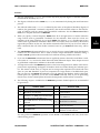
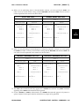
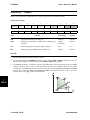
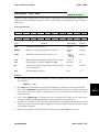
NEW FEATURES
Version 20.1 contains several new features as well as many minor enhancements and bug corrections. These features include:
☞
A new feature to perform automatic modal reductions, including Craig-Bampton, and
automatic static reduction. This feature allows models to be exported in the form of
DMIG Bulk Data entries. The exported models may then be use to couple structural
models from different sources. See Chapter 6 of the User’s Guide for complete
information.
UAI//NASTRAN
iii
User’s Reference Manual
☞
ARCHIVE Database. Extensions have been added to the ARCHIVE database. These
allow DMAP data block entities to be exported to, and imported from, DMAP solution
sequences. See DMAP Chapter of this manual.
☞
Equivalent Beam Forces. New feature for computing equivalent beam forces
(moments, shears, axial loads and torques) for sets of solid elements. See Chapter 5 of
the User’s Guide.
☞
Mode Tracking in Design Optimization. A new capability in Design Optimization
allows the automatic tracking of modes. This is important during the redesign
procedure to capture "mode swapping" as the design changes. See Chapter 26 of the
User’s Guide.
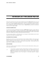
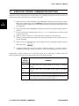
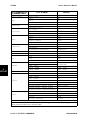
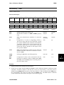
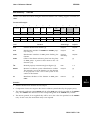
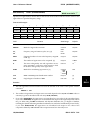
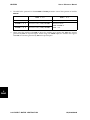
The following sections describe new features and modifications to UAI/NASTRAN input data.
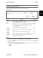
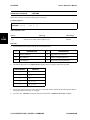
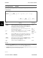
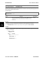
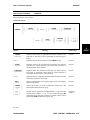
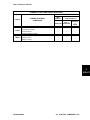
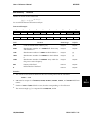
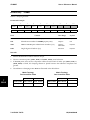
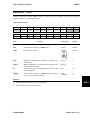
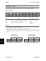
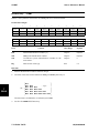
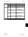
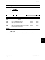
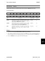
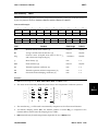
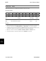
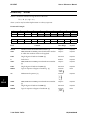
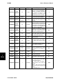
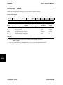
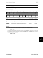
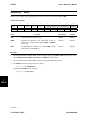
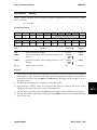
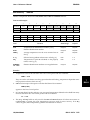
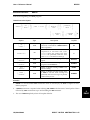
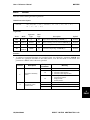
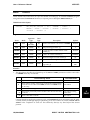
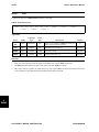
EXECUTIVE CONTROL PACKET
COMMAND
STAT
APPROACH
REV Clarification of the use of the various options.
ENTITY
DESCRIPTION
New feature for:
NEW - defining groups of database entities
- assigning groups to selected eBase databases.
SECONVERT
REV
Requests execution of a new version of the MSC/NASTRAN
Superelement convertor.
SEQUENCE
REV
New feature to select or deselect the inclusion of MPC and Rigid
Element data in the resequencing.
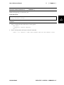
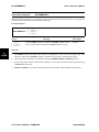
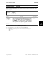
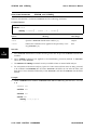
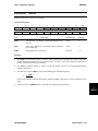
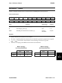
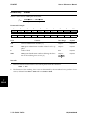
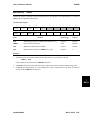
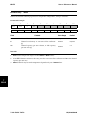
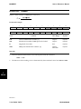
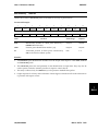
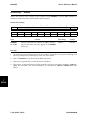
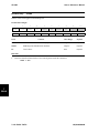
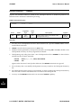
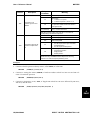
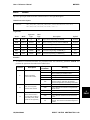
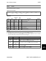
SUBSTRUCTURE CONTROL PACKET
COMMAND
COMBINE
STAT
DESCRIPTION
Enhanced to allow the new MATCH option for automatically
REV combining GRID points with identical identification numbers.
Especially useful in conjunction with the SECONVERT utility.
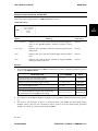
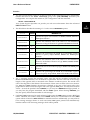
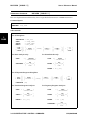
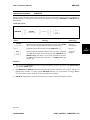
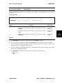
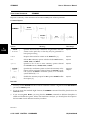
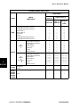
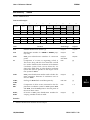
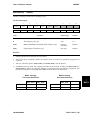
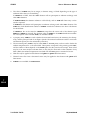
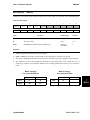
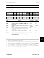
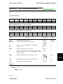
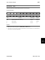
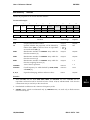
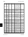
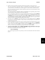
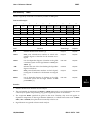
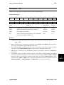
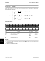
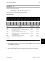
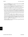
CASE CONTROL PACKET
COMMAND
STAT
AUTOREDUCE
NEW
New Command for automatic Guyan reduction of a model.
(See also NLREDUCE)
AUTOSPC
REV
New feature to select or deselect the application of AUTOSPC to
both the g-set and n-set for nonlinear analyses.
B2GG
B2PP
iv
DESCRIPTION
REV Extended to allow multiple direct input damping matrices.
UAI/NASTRAN
User’s Reference Manual
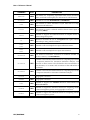
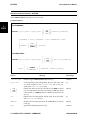
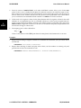
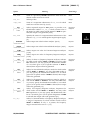
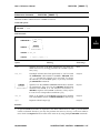
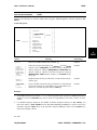
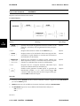
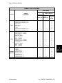
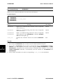
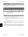
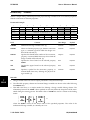
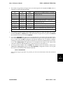
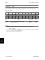
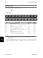
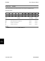
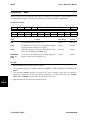
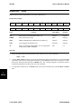
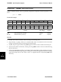
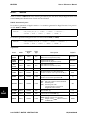
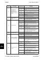
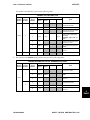
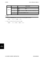
COMMAND
STAT
DESCRIPTION
BMFORCE
NEW
New feature for computing equivalent beam forces (moments,
shears, axial loads and torques) for collections of solid elements.
BOUNDARY
REV Extended for use with AUTOREDUCE and NLREDUCE
CASE
REV
New features to select automatic Guyan reduction or CraigBampton modal reduction.
EXPORT
NEW
New feature to export a reduced model as direct matrix input at
grid points (DMIG).
FORCE
REV
Extended to support the enhanced feature to compute forces at
element integration points.
IC
REV
Clarified to describe the use of the EQUILibrium option and its
relationship to using initial conditions.
K2GG
K2PP
REV Extended to allow multiple direct input stiffness matrices.
M2GG
M2PP
REV Extended to allow multiple direct input mass matrices.
New name for automatic reduction of nonlinear models. In
previous versions, was AUTOREDUCE.
NLREDUCE
REV
NLSTRAIN
Modified to describe the enhancements for computing layer strain
in composite material for Geometric Nonlinear analyses, and
REV extension to allow strains to be calculated at the extreme fibers of
plate elements, or as strains and curvatures at the midsurface of
the element.
NLSTRESS
REV
Modified to describe the enhancements for computing layer stress
in composite material for Geometric Nonlinear analyses.
NLTYPE
REV Typographic correction.
OMODES
REV Typographic correction.
POST
REV
Extended to support new OUPTUT2 interfaces with FEMAP and
UAI/RenderMaster.
STRAIN
REV
Extended to support the enhanced feature for computing strains
at element integration points, and typographic correction.
STRESS
REV
Extended to support the enhanced feature for computing stresses
at element integration points.
UAI//NASTRAN
v
User’s Reference Manual
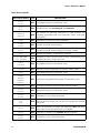
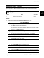
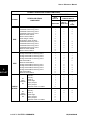
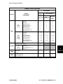
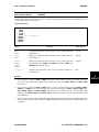
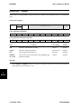
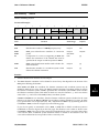
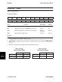
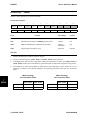
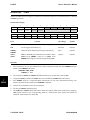
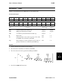
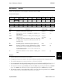
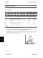
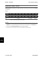
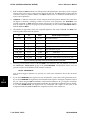
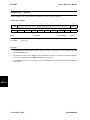
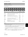
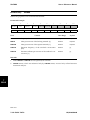
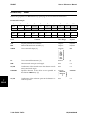
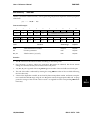
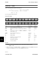
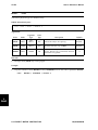
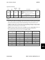
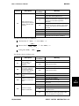
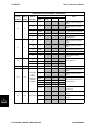
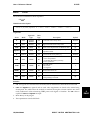
BULK DATA PACKET
BULK DATA ENTRY
ACCEL
ACCEL1
BDYS
BDYS1
BMFORCE
BMFORC1
CGAP
DESCRIPTION
REV Expanded description of orientation vector.
REV Extended for use with AUTOREDUCE and NLREDUCE.
New feature for defining collections of solid elements for
NEW computing equivalent beam forces (moments, shears, axial loads
and torques) .
REV Clarification of coordinate system definition.
DCFREQ
DCMODR
REV Extended to include mode tracking.
DVPROP
REV Extended to include modal damping as a design variable.
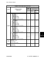
EIGC
EIGR (Lanczos)
EIGR (Givens)
REV Equations for damping computations corrected.
REV
Modified to allow specification of mass orthogonality test
parameter, E, in the Configuration File.
FORCE
FORCEAX
REV Expanded description of orientation vector.
FSIDATA
REV Enhanced to allow computation of free-free surface modes.
GRAV
REV Expanded description of orientation vector.
MOMAX
MOMENT
MOMENT1
MOMENT2
REV Corrections and expanded description of orientation vector.
NLSOLVE
REV Corrected to reflect the secant modulus solution method.
RFORCE
RFORCE1
REV Expanded description of orientation vector.
RLOAD1
RLOAD2
REV Clarification of use of enforced motion.
SETI
SETR
NEW
Entries that allow integer and real sets to be specified in the Bulk
Data packet.
SETOP
NEW
Allows set operations on integer sets defined by SETI Bulk Data
entries. Both Union and Intersection are available.
SHOCK
REV Correction to reference only TABLED1 Bulk data entries.
TLOAD1
TLOAD2
vi
STAT
REV Clarification of use of enforced motion.
UAI/NASTRAN
User’s Reference Manual
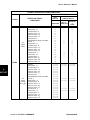
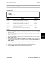
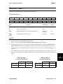
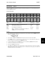
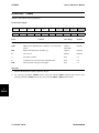
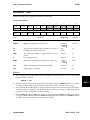
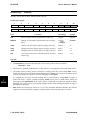
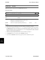
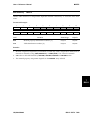
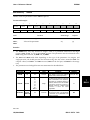
DMAP MODULES
MODULE NAME
DBIN
DBOUT
DBPARM
UAI//NASTRAN
STAT
DESCRIPTION
New modules used to import and export eBase entities when
REV using DMAP sequences. These are often used in conjunction with
the new Executive Control command ENTITY.
vii
User’s Reference Manual
This page is intentionally blank.
viii
UAI/NASTRAN
User’s Reference Manual
TABLE OF CONTENTS
FOREWORD . . . . . . . . . . . . . . . . . . . . . . . . . . . . . . . . . . . . . . . . . . . . . i
RELEASE NOTES . . . . . . . . . . . . . . . . . . . . . . . . . . . . . . . . . . . . . . . . . . iii
TABLE OF CONTENTS . . . . . . . . . . . . . . . . . . . . . . . . . . . . . . . . . . . . . . . ix
LIST OF FIGURES
. . . . . . . . . . . . . . . . . . . . . . . . . . . . . . . . . . . . . . . . xiii
LIST OF TABLES . . . . . . . . . . . . . . . . . . . . . . . . . . . . . . . . . . . . . . . . . xv
1. EXECUTING THE PROGRAM . . . . . . . . . . . . . . . . . . . . . . . . . . . . . . . . 1-1
1.1 OVERVIEW . . . . . . . . . . . . . . . . . . . . . . . . . . . . . . . . . . . . . . . . 1-2
1.1.1 Executing UAI/NASTRAN . . . . . . . . . . . . . . . . . . . . . . . . . . . 1-2
1.1.2 The UAI/NASTRAN Configuration and Preference Files . . . . . . . . . . 1-2
1.1.3 Executive Control Commands . . . . . . . . . . . . . . . . . . . . . . . . . 1-2
1.1.4 Dynamic Memory . . . . . . . . . . . . . . . . . . . . . . . . . . . . . . . . 1-3
1.1.5 The eBase Database . . . . . . . . . . . . . . . . . . . . . . . . . . . . . . 1-3
1.1.6 The INCLUDE Files
. . . . . . . . . . . . . . . . . . . . . . . . . . . . . . 1-4
1.1.7 UAI/NASTRAN Import/Export Files
1.1.8 Host Computer Dependencies
1.2 UNIX-BASED COMPUTERS
. . . . . . . . . . . . . . . . . . . . . 1-5
. . . . . . . . . . . . . . . . . . . . . . . . 1-6
. . . . . . . . . . . . . . . . . . . . . . . . . . . . . . 1-7
1.2.1 Executing UAI/NASTRAN . . . . . . . . . . . . . . . . . . . . . . . . . . . 1-7
1.2.2 UAI/NASTRAN File Names . . . . . . . . . . . . . . . . . . . . . . . . . . 1-8
1.2.3 ASSIGN and INCLUDE Command Parameters . . . . . . . . . . . . . . . 1-9
1.2.4 Site Definition of Automatic ASSIGN Commands . . . . . . . . . . . . . . 1-9
1.2.5 The eShell Program
. . . . . . . . . . . . . . . . . . . . . . . . . . . . . . 1-9
1.2.6 Automatic Preference Files . . . . . . . . . . . . . . . . . . . . . . . . . . 1-9
1.2.7 The Plotting Programs . . . . . . . . . . . . . . . . . . . . . . . . . . . . 1-10
1.2.8 Online Manuals . . . . . . . . . . . . . . . . . . . . . . . . . . . . . . . . 1-12
1.3 DEC VAX SERIES COMPUTERS — VMS OPERATING SYSTEM . . . . . . . . 1-13
1.3.1 Executing UAI/NASTRAN . . . . . . . . . . . . . . . . . . . . . . . . . . 1-13
UAI/NASTRAN
TABLE OF CONTENTS ix
User’s Reference Manual
1.3.2 UAI/NASTRAN File Names . . . . . . . . . . . . . . . . . . . . . . . . . 1-14
1.3.3 Monitoring the Execution . . . . . . . . . . . . . . . . . . . . . . . . . . . 1-15
1.3.4 ASSIGN and INCLUDE Command Parameters
. . . . . . . . . . . . . . 1-15
1.3.5 Site Definition of Automatic ASSIGN Commands . . . . . . . . . . . . . 1-16
1.3.6 Dynamic Memory . . . . . . . . . . . . . . . . . . . . . . . . . . . . . . . 1-16
1.3.7 The eShell Program . . . . . . . . . . . . . . . . . . . . . . . . . . . . . . 1-16
1.3.8 The Plotting Programs . . . . . . . . . . . . . . . . . . . . . . . . . . . . 1-16
1.3.9 Online Manuals . . . . . . . . . . . . . . . . . . . . . . . . . . . . . . . . 1-18
2. EXECUTIVE CONTROL COMMANDS . . . . . . . . . . . . . . . . . . . . . . . . . . . . 2-1
2.1 THE EXECUTIVE CONTROL COMMANDS . . . . . . . . . . . . . . . . . . . . . . 2-2
2.2 EXECUTIVE CONTROL SUBPACKETS . . . . . . . . . . . . . . . . . . . . . . . . 2-3
2.2.1 The ALTER Subpacket . . . . . . . . . . . . . . . . . . . . . . . . . . . . . 2-3
2.2.2 The DMAP Subpacket . . . . . . . . . . . . . . . . . . . . . . . . . . . . . 2-4
2.2.3 The RESTART Subpacket . . . . . . . . . . . . . . . . . . . . . . . . . . . 2-4
2.2.4 Configuration Parameters . . . . . . . . . . . . . . . . . . . . . . . . . . . 2-5
2.3 EXECUTIVE CONTROL COMMAND DESCRIPTIONS
. . . . . . . . . . . . . . . 2-6
3. SUBSTRUCTURE COMMANDS . . . . . . . . . . . . . . . . . .
3.1 THE SUBSTRUCTURE COMMANDS . . . . . . . . . . . . .
3.2 AUTOMATICALLY GENERATED DMAP ALTERS . . . . .
3.3 SUBSTRUCTURE TERMINOLOGY REVIEW . . . . . . . .
3.4 SUBSTRUCTURE CONTROL COMMAND DESCRIPTIONS
.
.
.
.
.
.
.
.
.
.
.
.
.
.
.
.
.
.
.
.
.
.
.
.
.
.
.
.
.
.
.
.
.
.
.
.
.
.
.
.
.
.
.
.
.
.
.
.
.
.
.
.
.
.
.
.
.
.
.
.
. 3-1
. 3-2
. 3-4
. 3-5
. 3-7
4. CASE CONTROL COMMANDS . . . . . . . . . . . . . . . . . . . . . . . . . . . . . . . . 4-1
4.1 CASE AND SUBCASE DEFINITION . . . . . . . . . . . . . . . . . . . . . . . . . . 4-3
4.1.1 Cases in the MULTI Solution Sequence . . . . . . . . . . . . . . . . . . . 4-3
4.2 DATA SELECTION . . . . . . . . . . . . . . . . . . . . . . . . . . . . . . . . . . . . 4-5
4.2.1 Load Selection
. . . . . . . . . . . . . . . . . . . . . . . . . . . . . . . . . 4-5
4.2.2 Temperature Field Selection
. . . . . . . . . . . . . . . . . . . . . . . . . 4-5
4.2.3 Constraints and Partitioning . . . . . . . . . . . . . . . . . . . . . . . . . . 4-5
4.2.4 Dynamics Control and Matrix Selection . . . . . . . . . . . . . . . . . . . 4-5
4.2.5 Multidisciplinary Design Optimization Control . . . . . . . . . . . . . . . . 4-5
4.2.6 Nonlinear Analysis Control
. . . . . . . . . . . . . . . . . . . . . . . . . . 4-5
4.2.7 Aerodynamic Analysis Control
. . . . . . . . . . . . . . . . . . . . . . . . 4-5
4.2.8 Fluid-Structure Interaction with Modal Synthesis . . . . . . . . . . . . . . 4-5
4.3 OUTPUT SELECTION . . . . . . . . . . . . . . . . . . . . . . . . . . . . . . . . . . 4-9
4.3.1 Output Control and Titling . . . . . . . . . . . . . . . . . . . . . . . . . . . 4-9
4.3.2 Defining Output Sets . . . . . . . . . . . . . . . . . . . . . . . . . . . . . . 4-9
4.3.3 Solution Results . . . . . . . . . . . . . . . . . . . . . . . . . . . . . . . . 4-10
4.3.4 Exporting Data
. . . . . . . . . . . . . . . . . . . . . . . . . . . . . . . . 4-10
4.4 DEFINING ANALYSIS CASES
. . . . . . . . . . . . . . . . . . . . . . . . . . . . 4-12
4.4.1 CASE (or SUBCASE) Specifications . . . . . . . . . . . . . . . . . . . . 4-12
4.5 MINIMAL REQUIRED CASE CONTROL COMMANDS . . . . . . . . . . . . . . . 4-13
4.6 COMMONLY USED OPTIONS . . . . . . . . . . . . . . . . . . . . . . . . . . . . 4-14
x TABLE OF CONTENTS
UAI/NASTRAN
User’s Reference Manual
4.6.1 SORT1 and SORT2 . . . . . . . . . . . . . . . . . . . . . . . . . . . . . . 4-14
4.6.2 PRINT and NOPRINT (POST) . . . . . . . . . . . . . . . . . . . . . . . . 4-14
4.6.3 RECTANGULAR and POLAR
. . . . . . . . . . . . . . . . . . . . . . . . . 4-16
4.6.4 Output Set Selection . . . . . . . . . . . . . . . . . . . . . . . . . . . . . 4-16
4.6.5 Configuration Parameters . . . . . . . . . . . . . . . . . . . . . . . . . . 4-17
4.7 COMPATIBILITY WITH OTHER SYSTEMS . . . . . . . . . . . . . . . . . . . . . 4-18
4.7.1 The AUTOSPC Feature . . . . . . . . . . . . . . . . . . . . . . . . . . . . 4-18
4.7.2 The AUTOOMIT Feature . . . . . . . . . . . . . . . . . . . . . . . . . . . 4-18
4.8 CASE CONTROL COMMAND DESCRIPTIONS . . . . . . . . . . . . . . . . . . . 4-19
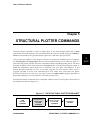
5. STRUCTURAL PLOTTER COMMANDS . . . . . .
5.1 THE STRUCTURAL PLOTTER COMMANDS
5.2 STRUCTURAL PLOTTING TERMINOLOGY .
5.3 SET DEFINITION . . . . . . . . . . . . . . . .
5.4 VIEWING OPTION COMMANDS . . . . . . .
.
.
.
.
.
.
.
.
.
.
.
.
.
.
.
.
.
.
.
.
.
.
.
.
.
.
.
.
.
.
.
.
.
.
.
.
.
.
.
.
.
.
.
.
.
.
.
.
.
.
.
.
.
.
.
.
.
.
.
.
.
.
.
.
.
.
.
.
.
.
.
.
.
.
.
.
.
.
.
.
.
.
.
.
.
.
.
.
.
.
.
.
.
.
.
.
.
.
.
.
.
.
.
.
.
5-1
5-2
5-4
5-6
5-8
5.4.1 Viewing Angles . . . . . . . . . . . . . . . . . . . . . . . . . . . . . . . . . 5-8
5.4.2 The Graphics Projection . . . . . . . . . . . . . . . . . . . . . . . . . . . 5-10
5.4.3 ZOOMing
5.5
5.6
5.7
5.8
5.9
. . . . . . . . . . . . . . . . . . . . . . . . . . . . . . . . . . . 5-10
PLOTTING THE MODEL GEOMETRY
PLOTTING SOLUTION RESULTS . .
ASSIGNING FILES . . . . . . . . . . .
DEVICE COMMANDS . . . . . . . . .
STRUCTURAL PLOTTER COMMAND
. . . . . . . . . .
. . . . . . . . . .
. . . . . . . . . .
. . . . . . . . . .
DESCRIPTIONS
.
.
.
.
.
.
.
.
.
.
.
.
.
.
.
.
.
.
.
.
.
.
.
.
.
.
.
.
.
.
.
.
.
.
.
.
.
.
.
.
.
.
.
.
.
.
.
.
.
.
.
.
.
.
.
.
.
.
.
.
.
.
.
.
.
.
.
.
.
.
5-11
5-12
5-14
5-15
5-16
6. X-Y PLOTTER COMMANDS . . . . . . . . . . . . . . . . . . . . . . . . . . . . . . . . . 6-1
6.1 THE X-Y PLOTTER COMMANDS . . . . . . . . . . . . . . . . . . . . . . . . . . . 6-3
6.1.1 The X-Y Plotter Functions . . . . . . . . . . . . . . . . . . . . . . . . . . . 6-3
6.1.2 ASSIGNing Files . . . . . . . . . . . . . . . . . . . . . . . . . . . . . . . . 6-3
6.1.3 Specifying Plotter Controls . . . . . . . . . . . . . . . . . . . . . . . . . . 6-4
6.1.4 The Plot Elements . . . . . . . . . . . . . . . . . . . . . . . . . . . . . . . 6-4
6.1.5 Plot Titling . . . . . . . . . . . . . . . . . . . . . . . . . . . . . . . . . . . . 6-4
6.1.6 Data Scaling
. . . . . . . . . . . . . . . . . . . . . . . . . . . . . . . . . . 6-4
6.1.7 Selecting SUBCASES . . . . . . . . . . . . . . . . . . . . . . . . . . . . . 6-9
6.1.8 Defining Frames and Curves . . . . . . . . . . . . . . . . . . . . . . . . . 6-9
6.2 SOLUTION RESPONSE CODES . . . . . . . . . . . . . . . . . . . . . . . . . . . 6-11
6.3 X-Y PLOTTER COMMAND DESCRIPTIONS . . . . . . . . . . . . . . . . . . . . 6-27
7. BULK DATA . . . . . . . . . . . . . . . . . . . . . . . . . . . . . . . . . . . . . . . . . . 7-1
7.1 FORMAT OF BULK DATA ENTRIES . . . . . . . . . . . . . . . . . . . . . . . . . . 7-2
7.1.1 Free-Field Data Entry . . . . . . . . . . . . . . . . . . . . . . . . . . . . . 7-2
7.1.2 Fixed-Field Data Entry . . . . . . . . . . . . . . . . . . . . . . . . . . . . . 7-5
7.1.3 High-Precision Data Entry
. . . . . . . . . . . . . . . . . . . . . . . . . . 7-6
7.1.4 Integer List Data Entry . . . . . . . . . . . . . . . . . . . . . . . . . . . . . 7-7
7.2 AUTOMATIC DATA GENERATION . . . . . . . . . . . . . . . . . . . . . . . . . . . 7-8
7.2.1 TEMPLATE Entries
UAI/NASTRAN
. . . . . . . . . . . . . . . . . . . . . . . . . . . . . . 7-8
TABLE OF CONTENTS xi
User’s Reference Manual
7.2.2 REPLICATION Entries . . . . . . . . . . . . . . . . . . . . . . . . . . . . . 7-8
7.2.3 COUNTER Entries . . . . . . . . . . . . . . . . . . . . . . . . . . . . . . 7-10
7.2.4 Replication Examples
. . . . . . . . . . . . . . . . . . . . . . . . . . . . 7-10
7.2.5 Restrictions on Replication
7.3 BULK DATA DESCRIPTIONS
. . . . . . . . . . . . . . . . . . . . . . . . . 7-11
. . . . . . . . . . . . . . . . . . . . . . . . . . . . 7-12
7.3.1 Format and Examples . . . . . . . . . . . . . . . . . . . . . . . . . . . . 7-12
7.3.2 Field Definitions . . . . . . . . . . . . . . . . . . . . . . . . . . . . . . . . 7-13
7.3.3 Remarks . . . . . . . . . . . . . . . . . . . . . . . . . . . . . . . . . . . . 7-14
7.3.4 Usage
. . . . . . . . . . . . . . . . . . . . . . . . . . . . . . . . . . . . . 7-14
8. DIRECT MATRIX ABSTRACTION . . . . .
8.1 DMAP INSTRUCTIONS . . . . . . . .
8.2 DATA FLOW IN UAI/NASTRAN . . . .
8.3 DMAP INSTRUCTION SYNTAX . . .
.
.
.
.
.
.
.
.
.
.
.
.
.
.
.
.
.
.
.
.
.
.
.
.
.
.
.
.
.
.
.
.
.
.
.
.
.
.
.
.
.
.
.
.
.
.
.
.
.
.
.
.
.
.
.
.
.
.
.
.
.
.
.
.
.
.
.
.
.
.
.
.
.
.
.
.
.
.
.
.
.
.
.
.
.
.
.
.
.
.
.
.
.
.
.
.
.
.
.
.
8-1
8-2
8-3
8-4
8.3.1 Syntax of Functional Module Instructions . . . . . . . . . . . . . . . . . . 8-4
8.3.2 Syntax of Executive Instructions . . . . . . . . . . . . . . . . . . . . . . . 8-6
8.4 EXAMPLES OF DMAP . . . . . . . . . . . . . . . . . . . . . . . . . . . . . . . . . . 8-7
8.4.1 Solving Matrix Equations . . . . . . . . . . . . . . . . . . . . . . . . . . . . 8-7
8.4.2 Looping in DMAP Programs . . . . . . . . . . . . . . . . . . . . . . . . . . 8-8
8.4.3 Partitioning Operations and ALTERs . . . . . . . . . . . . . . . . . . . . . 8-8
8.4.4 Testing and Branching with DMAP . . . . . . . . . . . . . . . . . . . . . . 8-9
8.5 DMAP MODULE DESCRIPTIONS
xii TABLE OF CONTENTS
. . . . . . . . . . . . . . . . . . . . . . . . . . 8-10
UAI/NASTRAN
User’s Reference Manual
LIST OF FIGURES
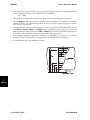
2. EXECUTIVE CONTROL COMMANDS . . . . . . . . . . . . . . . . . . . . . . . . . . . 2-1
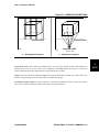
Figure 2-1. EXECUTIVE CONTROL PACKET LOCATION . . . . . . . . . . . . . . . . 2-1
3. SUBSTRUCTURE COMMANDS
. . . . . . . . . . . . . . . . . . . . . . . . . . . . . . 3-1
Figure 3-1. SUBSTRUCTURE CONTROL PACKET LOCATION . . . . . . . . . . . . . 3-1
Figure 3-2. SUBSTRUCTURING ANALYSIS TREE . . . . . . . . . . . . . . . . . . . . 3-5
4. CASE CONTROL COMMANDS . . . . . . . . . . . . . . . . . . . . . . . . . . . . . . . 4-1
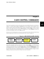
Figure 4-1. CASE CONTROL PACKET LOCATION . . . . . . . . . . . . . . . . . . . . 4-1
Figure 4-2. COMPLEX OUTPUT REPRESENTATIONS . . . . . . . . . . . . . . . . . 4-16
5. STRUCTURAL PLOTTER COMMANDS . . . . . . . . . .
Figure 5-1. THE STRUCTURAL PLOTTER SUBPACKET
Figure 5-2. PLOTTER COORDINATE SYSTEM . . . . . .
Figure 5-3. GRAPHIC PROJECTIONS . . . . . . . . . . .
Figure 5-4. BASIC PLOT ELEMENTS . . . . . . . . . . . .
Figure 5-5. USING THE AXES COMMAND . . . . . . . . .
Figure 5-6. SOLUTION RESULTS PLOTS . . . . . . . . .
.
.
.
.
.
.
.
.
.
.
.
.
.
.
.
.
.
.
.
.
.
.
.
.
.
.
.
.
.
.
.
.
.
.
.
.
.
.
.
.
.
.
.
.
.
.
.
.
.
.
.
.
.
.
.
.
.
.
.
.
.
.
.
.
.
.
.
.
.
.
.
.
.
.
.
.
.
.
.
.
.
.
.
.
.
.
.
.
.
.
.
.
.
.
.
.
.
.
.
.
.
.
.
.
.
. 5-1
. 5-1
. 5-4
. 5-5
. 5-8
. 5-9
5-12
6. X-Y PLOTTER COMMANDS
. . . . . . . . . . . . . . . . . .
Figure 6-1. LOCATION OF THE X-Y PLOTTER SUBPACKET
Figure 6-2. PLOT ELEMENTS FOR WHOLE FRAMES . . . .
Figure 6-3. PLOT ELEMENTS FOR HALF FRAMES . . . . .
.
.
.
.
.
.
.
.
.
.
.
.
.
.
.
.
.
.
.
.
.
.
.
.
.
.
.
.
.
.
.
.
.
.
.
.
.
.
.
.
.
.
.
.
.
.
.
.
.
.
.
.
.
.
.
.
6-1
6-1
6-7
6-8
7. BULK DATA . . . . . . . . . . . . . . . . . . . . . . . . . . . . . . . . . . . . . . . . . . 7-1
Figure 7-1. BULK DATA PACKET LOCATION . . . . . . . . . . . . . . . . . . . . . . . 7-1
UAI/NASTRAN
xiii
User’s Reference Manual
This page is intentionally blank.
xiv
UAI/NASTRAN
User’s Reference Manual
LIST OF TABLES
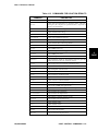
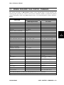
2. EXECUTIVE CONTROL COMMANDS . . . . . . . . . . . . . . . . . . . . . . . . . . . . 2-1
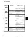
Table 2-1. SUMMARY OF EXECUTIVE CONTROL COMMANDS . . . . . . . . . . . . 2-2
3. SUBSTRUCTURE COMMANDS . . . . . . . . . . . . . . . . . . . . . . . . . . . . . . . 3-1
Table 3-1. SUMMARY OF SUBSTRUCTURE CONTROL COMMANDS . . . . . . . . . 3-3
4. CASE
Table
Table
Table
Table
Table
Table
Table
Table
Table
Table
Table
Table
Table
Table
CONTROL COMMANDS . . . . . . . . . . . . . . . . . . . . . .
4-1. COMMANDS FOR CASE AND SUBCASE DEFINITION . .
4-2. COMMANDS FOR LOAD SELECTION . . . . . . . . . . . .
4-3. COMMANDS FOR TEMPERATURE FIELD SELECTION .
4-4. COMMANDS FOR CONSTRAINT SELECTION . . . . . . .
4-5. COMMANDS FOR DYNAMICS CONTROL . . . . . . . . .
4-6. COMMANDS FOR MDO . . . . . . . . . . . . . . . . . . . .
4-7. COMMANDS FOR NONLINEAR MATERIAL ANALYSIS . .
4-8. COMMANDS FOR AERODYNAMIC ANALYSIS CONTROL
4-9. COMMANDS FOR FSI - MODAL SYNTHESIS . . . . . . .
4-10. COMMANDS FOR GENERAL OUTPUT SELECTION . . .
4-11. COMMANDS FOR SET DEFINITION . . . . . . . . . . . .
4-12. COMMANDS FOR DATA EXPORT . . . . . . . . . . . . .
4-13. COMMANDS FOR SOLUTION RESULTS . . . . . . . . .
4-14. OUTPUT SORT ORDER FOR RIGID FORMATS . . . . .
.
.
.
.
.
.
.
.
.
.
.
.
.
.
.
.
.
.
.
.
.
.
.
.
.
.
.
.
.
.
.
.
.
.
.
.
.
.
.
.
.
.
.
.
.
.
.
.
.
.
.
.
.
.
.
.
.
.
.
.
.
.
.
.
.
.
.
.
.
.
.
.
.
.
.
.
.
.
.
.
.
.
.
.
.
.
.
.
.
.
.
.
.
.
.
.
.
.
.
.
.
.
.
.
.
.
.
.
.
.
.
.
.
.
.
.
.
.
.
.
. 4-1
. 4-3
. 4-6
. 4-6
. 4-6
. 4-7
. 4-7
. 4-7
. 4-8
. 4-8
. 4-9
. 4-9
4-10
4-11
4-15
5. STRUCTURAL PLOTTER COMMANDS . . . . . . . . . . . . . . . . . . . . . . . . . . . 5-1
Table 5-1. SUMMARY OF STRUCTURAL PLOTTER COMMANDS . . . . . . . . . . . 5-3
UAI/NASTRAN
xv
User’s Reference Manual
6. X-Y PLOTTER COMMANDS . . . . . .
Table 6-1. X-Y PLOTTER FUNCTIONS
Table 6-2. X-Y PLOTTER COMMANDS
Table 6-3. X-Y PLOTTER COMMANDS
Table 6-4. X-Y PLOTTER COMMANDS
Table 6-5. X-Y PLOTTER COMMANDS
. . .
. . .
FOR
FOR
FOR
FOR
. . . . . . . . . . . . . .
. . . . . . . . . . . . . .
POST-PROCESSORS
PLOT ELEMENTS . . .
TITLING . . . . . . . .
DATA SCALING . . . .
.
.
.
.
.
.
.
.
.
.
.
.
.
.
.
.
.
.
.
.
.
.
.
.
.
.
.
.
.
.
.
.
.
.
.
.
.
.
.
.
.
.
.
.
.
.
.
.
.
.
.
.
.
.
.
.
.
.
.
.
6-1
6-3
6-4
6-5
6-5
6-6
8. DIRECT MATRIX ABSTRACTION . . . . . . . . . . . . . . . . . . . . . . . . . . . . . . 8-1
Table 8-1. DMAP MODULES FOR GENERAL USE . . . . . . . . . . . . . . . . . . . . 8-2
Table 8-2. PREFACE eBase ENTITY NAMES . . . . . . . . . . . . . . . . . . . . . . . 8-3
xvi
UAI/NASTRAN
User’s Reference Manual
1
JCL
Chapter 1
EXECUTING THE PROGRAM
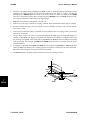
As is the case with all major software systems that are available across a broad spectrum of host
computers and operating systems†, UAI/NASTRAN has features that are implemented differently
on different computers. The most common differences are in the way that you execute UAI/NASTRAN and other UAI software products, the management of dynamic memory, and the manner in
which files are handled during execution.
☞
†
Information describing interfaces with third-party software such as MSC/PATRAN ®
and SDRC I-DEAS® is found in Chapter 31 of the UAI/NASTRAN User’s Guide.
All computer models and operating system names are trademarks of their respective manufacturers and vendors.
Rev: V20.1
UAI/NASTRAN
EXECUTING THE PROGRAM 1-1
User’s Reference Manual
1.1
1
JCL
OVERVIEW
This section provides you with an overview of the areas of UAI/NASTRAN that are directly affected
by your host computer and its operating system.
1.1.1
Executing UAI/NASTRAN
The manner in which you invoke a UAI/NASTRAN execution is completely dependent on the
operating system of your host computer. Subsequent sections of this chapter describe this operation
for the most common host computers upon which UAI/NASTRAN is currently available. You will
note that Section 1.2 includes all of the host computers using the Unix operating system and its
derivatives.
1.1.2
The UAI/NASTRAN Configuration and Preference Files
In general, UAI’s suite of engineering software products uses computing resources intensively. As a
result, there are a number of parameters that must be set to achieve optimal resource management
on a given host computer. These parameters, taken as a group, are called the Configuration of the
products. The configuration is provided through several files. These files include parameters which
are used for controlling such things as database locations, physical file characteristics, memory
utilization, and algorithm control.
For maximum flexibility, configurations may be controlled both by the site, i.e. the UAI System
Support Specialist for larger companies, and the end user. Many different configurations may be
defined for a site or a user. For example, when configuring UAI/NASTRAN, the UAI System Support Specialist may create different configurations for very small and for very large analyses.
Among the most common reasons reasons for having a customized configuration are:
1.1.3
❒
To allocate large amounts of memory and CPU time limits, by default, when always
executing large analyses.
❒
To define the locations of file systems when databases are expected to exceed 2GB in size.
❒
To make engineering options ( e.g. AUTOSPC and AUTOOMIT) compatible with other
NASTRAN variants.
❒
To select comprehensive data checking options which have more stringent tests than other
NASTRAN variants (e.g. element warping and aspect ratio checks).
Executive Control Commands
Chapter 2 of this manual presents the UAI/NASTRAN Executive Control commands. These commands provide general information to UAI/NASTRAN during execution. While the great majority
of these commands are implemented in a host-independent manner, there are two commands
which do depend on your host computer. The first of these, ASSIGN, is used to attach physical files
on your host computer to logical files within UAI/NASTRAN. The second of these commands is
INCLUDE. You use this command to insert a text file into your UAI/NASTRAN input data stream.
Descriptions of all host-dependent data that are required are discussed in following sections.
1-2 EXECUTING THE PROGRAM
UAI/NASTRAN
User’s Reference Manual
1.1.4
Dynamic Memory
The architecture of UAI/NASTRAN allows the modeling and analysis of finite element models of
virtually unlimited size. Most numerical calculations perform at maximum efficiency when all data
for the operation fits in the working memory space of the program. Many operations may be
performed even when all data that they require does not fit in memory by using what is called spill
logic. Spill logic simply involves the paging of data to and from disk storage devices as necessary.
For very large jobs, spill commonly occurs. In such cases, providing UAI/NASTRAN with additional
working memory can often improve performance. On the other hand, you do not want to give
UAI/NASTRAN excess memory, because it will reduce resources that could be used for other processes on your system. Under certain circumstances, excess memory may actually degrade the performance of UAI/NASTRAN and, in extreme cases, even your computer system.
UAI/NASTRAN has a second independent dynamic memory which is used to operate on databases
that are attached to the execution. This memory is typically much smaller than the working memory. The main factor influencing the amount of database memory required is the block size used by
the active databases. This is described in detail in subsequent sections.
The working memory for UAI/NASTRAN is dynamically acquired during execution. The amount of
space that is actually used by the program is typically controlled by the UAI/NASTRAN execution
procedure or the MEMORY Executive Control command. Some host computers have alternate means
of controlling this memory.
1.1.5
The eBase Database
With UAI/NASTRAN Version 11.0, UAI introduced the Engineering Database Management System,
eBase, into UAI/NASTRAN. This advanced scientific database technology greatly enhances the data
handling capabilities of UAI/NASTRAN while removing many of the inconveniences of the older
I/O system which used sequential files.
The Three Types of Databases
There are three types of eBase databases. The first is the system database. This is used by UAI/NASTRAN to store items such as error message text and database schemata definitions. The second type
is the run-time database, or RUNDB. This database is used to store the relations and matrices which
are used in performing your analysis task. At the end of your job, the RUNDB is deleted. The third
type is the archival database. This type of database is saved from one execution to the next. There
are three archival databases. The first is the SOF database, used in performing Substructuring
Analyses, and the second is the NLDB database, used when you perform Nonlinear Material or
Geometry Analyses. The third database is the Archive database which is controlled by the ARCHIVE
Case Control command. This database may contain the geometry and solution results for your run
in easy-to-use relational form. The format, or schema, of these relations is described in the
UAI/NASTRAN Archive Database Manual.
The Logical and Physical Views of the Database
To fully understand the database technology, you must understand the two views of the database.
Each database is called a logical database. This term is used because from an engineering viewpoint, the database is a single entity which is used in its entirety. The manner in which the logical
database is stored on your host computer depends on the amount of data it contains and the
availability of disk storage devices. The physical view is a mapping of a logical database to some
UAI/NASTRAN
EXECUTING THE PROGRAM 1-3
1
JCL
User’s Reference Manual
1
JCL
number of physical files on your host computer. It may be necessary for you to understand the
physical model because, for very large analyses, it may be more efficient to organize the actual files
in a manner that allows higher performance on your host computer.
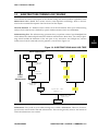
The Physical Model
Each eBase database, regardless of its use, has two components manifested as a minimum of two
physical files. The first of these components is called the INDEX component. This component is
always a single physical file. It contains information which identifies and locates actual database
entities. These entities themselves are stored in the DATA component. To provide the maximum
flexibility for a wide variety of data storage requirements, the data components may be stored in a
number of different physical files. Most database systems are organized in this manner, because the
index component is generally small in size and referenced often, while the data component may be
extremely large and not fit in a single file or even on a single disk drive.
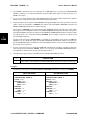
ASSIGNing Databases
Each logical database must be defined using the Executive Control command ASSIGN. The general
form of the ASSIGN command is:
NEW
ASSIGN logical_name [= phys_name] , OLD [,USE = use][,REALLOC]
TEMP
[,PASSWORD = pass][,IBLKSIZE = nwib][,DBLKSIZE = nwdb]
[,ACCESS = access][,params]
The description of the ASSIGN command for databases, as well as other files, is found in Chapter 2
of this manual. Of interest here are the optional params. The meaning and availability of these
params depends on the UAI/NASTRAN host computer. When available, these are described for
each computer beginning in Section 1.2 of this chapter.
Database File Names
The naming of database files follows a convention that is different from that of other UAI/NASTRAN files. The file names are generated automatically at execution time. The conventions used are
also described starting in Section 1.2 of this chapter.
Very Large Databases
You may be solving extremely large problems with UAI/NASTRAN. In such cases it may be possible that a databases exceeds the capacity of a single disk drive. UAI/NASTRAN has made provision
for this and you must contact your UAI/NASTRAN System Support Specialist for details describing
the use of this advanced feature.
1.1.6
The INCLUDE Files
To simplify the creation of the UAI/NASTRAN input data stream, you may insert files directly into
the input stream by using the INCLUDE command which may appear in any of the data packets.
The general syntax of this command is:
1-4 EXECUTING THE PROGRAM
UAI/NASTRAN
User’s Reference Manual
INCLUDE filename [,params]
As in the case of the ASSIGN command, on some host computers there are additional params which
may be used. These are also described starting in Sections 1.2 of this chapter. Note that INCLUDE
commands may appear in any position within your input data stream.
1.1.7
UAI/NASTRAN Import/Export Files
There are a number of file-based operations that are frequently performed when using UAI/NASTRAN. These are described in the following sections.
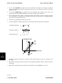
Using the INPUTT2/OUTPUT2 and INPUTT4/OUTPUT4 Modules
UAI/NASTRAN provides modules with which you may import data into, or export data from, the
program in a form which may be interfaced to FORTRAN programs. Typically, you use these
features for pre- and post-processing of data. When using the INPUTT2 and OUTPUT2 modules, the
files are written using FORTRAN variable length, unformatted or binary records. The INPUTT4 and
OUTPUT4 allow you to read or write data in either of two ways. You control your selection with the
parameter TYPE. The two types, FORMATTED and BINARY, determine the type of FORTRAN I/O
used to process the file.
Either the files used by these modules must be allocated and assigned by using the ASSIGN Executive Control command for a logical file with a USE parameter specifying the appropriate module, or
they may use the default parameters available under automatic ASSIGNment. A detailed description of the format of these files is found in Chapter 8 of this manual.
Using the SOFIN and SOFOUT Modules
The substructuring capability within UAI/NASTRAN uses an archival database called the SOF.
There are two utility operations which you may perform on an SOF database. The first of these is
called SOFOUT. This operation is used to export an SOF database from your UAI/NASTRAN job.
The second operation is called SOFIN. This operation allows you to import a file which contains an
SOF database that was exported during a previous execution.
These operations may be performed in either of two modes. The first mode is called the INTERNAL
format. When you create an export file using SOFOUT with a TYPE of INTERNAL, the file is created
with FORTRAN binary I/O. It may therefore be imported into another UAI/NASTRAN execution
only on the same host computer or another computer which is fully compatible with the computer
on which it was created. The second mode is called the EXTERNAL format. When you create an
export file using SOFOUT with a TYPE of EXTERNAL, the file is created with formatted FORTRAN
I/O. In this case, it may be imported into another UAI/NASTRAN execution on any host computer.
As a result, the EXTERNAL format can be used to transfer SOF data between one type of host
computer and another. This can be done by either creating a tape on your host which will be
physically loaded on the other computer, or by transferring the data directly over a network.
The NASTPLOT File
UAI/NASTRAN provides extensive plotting capability both for structural plots and X-Y plots of
solution results. These capabilities are described in detail in Chapters 5 and 6 of this manual. When
you use either, or both, of these features, you may ASSIGN a file with a USE of PLOT, or use the
automatic ASSIGNment default. In a manner similar to that described in the previous two sections,
UAI/NASTRAN
EXECUTING THE PROGRAM 1-5
1
JCL
User’s Reference Manual
1
JCL
you may select a TYPE of either FORMATTED or BINARY for this file. You select the BINARY option
when your NASTPLOT post-processor program will be executed on your UAI/NASTRAN host
computer. If your NASTPLOT program resides on a different computer, then you must use the
FORMATTED option to facilitate the transfer of data from the UAI/NASTRAN host to the NASTPLOT
host. In addition, UAI provides certain display capabilities for each host computer. These are
described in the remainder of this Chapter.
1.1.8
Host Computer Dependencies
The sections that follow provide detailed information describing the differences in UAI/NASTRAN
execution procedures and commands which depend on your host computer system.
1-6 EXECUTING THE PROGRAM
UAI/NASTRAN
User’s Reference Manual
1.2
UNIX-BASED COMPUTERS
This section describes the host-dependent information that you need to execute UAI/NASTRAN on
Unix-based computer systems. UAI supports a wide variety of these computers including those
manufactured by Cray, DEC, HP, IBM, SGI, Sun and others. For a complete list of platforms, please
contact UAI.
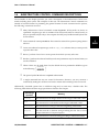
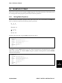
1.2.1
Executing UAI/NASTRAN
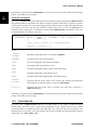
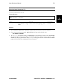
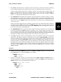
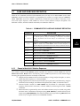
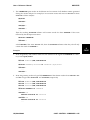
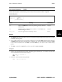
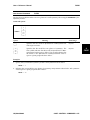
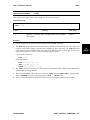
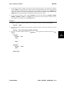
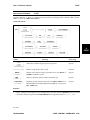
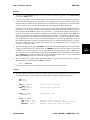
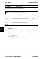
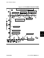
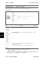
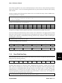
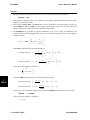
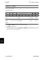
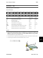
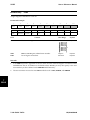
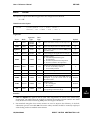
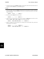
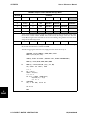
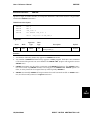
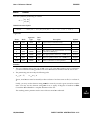
A csh script file, called nastran, is provided to execute UAI/NASTRAN. To execute you enter:
nastran −m
W
memory K P [-ps prefname] [-pu prefname]
M B
[-pl prefname] filelist
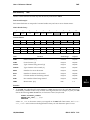
where memory specifies the amount of memory that the job will use. Options allow you to use
shorthand notation for large values and allocation types. The options K and M indicate that the
memory value is specified in thousands or millions of units, respectively. The units may be specified in single precision words (W), bytes (B), or machine precision words (P). If none of these
arguments are used, then memory is assumed to be single precision words. The prefname specifies the substitution string used to generate preference File names. You may specify a different
string for the system (-ps), the user (-pu) and the local (-pl) preference files. If you have the
unusual case where all of these files have the same name, you may use the option -p followed by
the prefname. Finally, filelist specifies a list of one or more file names, separated by spaces,
that contain UAI/NASTRAN input data streams. The actual file names must have the proper trailing
component, which is usually .d. The script file will execute UAI/NASTRAN using each of the data
files that you provide. Examples illustrating the use of the script are shown below.
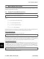
1.
Execute UAI/NASTRAN using the input file test.d
nastran test
2.
Execute UAI/NASTRAN in the background for all of the input files in directory
/uai/demodata.
nastran /uai/demodata/*.d &
3.
Execute UAI/NASTRAN using the input file test.d and request one million words of memory.
nastran -m 1000000 test or
nastran -m 1mw test or
nastran -m 1000kw test
UAI/NASTRAN
EXECUTING THE PROGRAM 1-7
1
JCL
User’s Reference Manual
4.
1
JCL
Suppose that you have created a Preference File name my.pref, execute UAI/NASTRAN using
the input file test.d using these preferences.
nastran -p my test
1.2.2
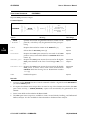
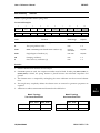
UAI/NASTRAN File Names
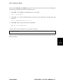
When you execute the nastran script a number of files may be created which have names that are
automatically generated by the program. These are described in this section.
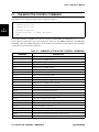
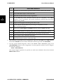
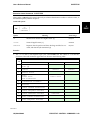
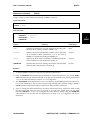
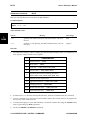
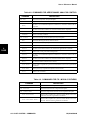
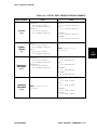
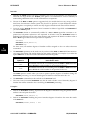
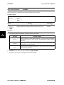
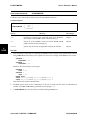
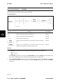
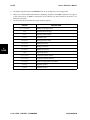
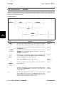
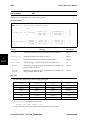
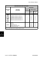
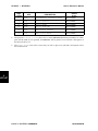
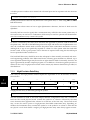
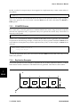
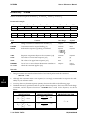
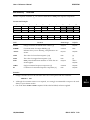
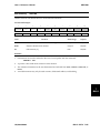
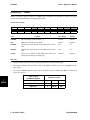
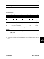
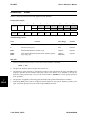
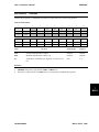
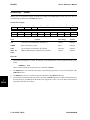
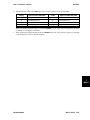
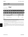
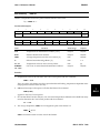
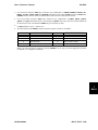
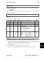
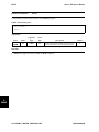
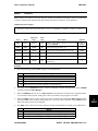
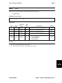
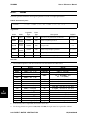
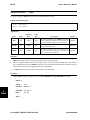
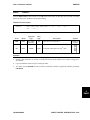
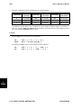
Unique UAI/NASTRAN files
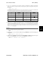
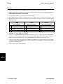
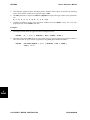
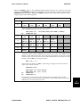
There are four unique files that are used frequently by UAI/NASTRAN. These are unique in the
sense the program will automatically define file names for these if you do not explicitly ASSIGN
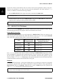
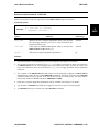
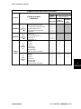
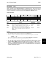
them. These files, and their default names, are shown in the table below:
FILE
May Override with
ASSIGN Command?
Generated Name if ASSIGN
Command is Not Used
The print file
NO
filename.prt
The log file
NO
filename.log
The BULK file
YES
filename.bulk
The PUNCH file
YES
filename.pch
The filename represents the name of the file containing the UAI/NASTRAN input data stream.
The log file is a special file that contains the history of your execution. You may monitor the
progress of your job by viewing the log file periodically. Upon completion of the job, the log file is
appended to the print file, and then deleted.
Databases
You will recall from Section 1.1.4 that each database that you use during an execution is comprised
of at least two physical files. The trailing components of these file names is always generated by
UAI/NASTRAN. When you ASSIGN a database with a status of NEW and provide a physical file
name, phys_name, the program generates the file names:
phys_name.edb and phys_name.00
There may be times, most often in the case of the RUNDB, that you ASSIGN a database with a status
of TEMP. In such cases, the program internally generates file names that are unique to your job. The
detailed rules used to generate these names are given in the System Support Manual. These simple
rules pertain to the simplest and most used ASSIGNments of databases. If you are using very large
databases, then there are additional rules. These will be provided by your UAI/NASTRAN System
Support Specialist.
1-8 EXECUTING THE PROGRAM
UAI/NASTRAN
User’s Reference Manual
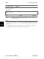
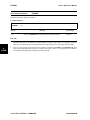
1.2.3
ASSIGN and INCLUDE Command Parameters
There are no additional parameters for the INCLUDE command for Unix-based host computers. The
ASSIGN command has two special parameters, ILOC and DLOC, that are used to control the location of the physical files comprising a database. Contact your UAI/NASTRAN System Support
Specialist for a complete description of how these parameters are used.
1.2.4
Site Definition of Automatic ASSIGN Commands
UAI/NASTRAN provides a capability which allows an individual client site to define a set of ASSIGN commands which are used automatically by the program as needed. When this feature is
used, it is not necessary for you to specify your own ASSIGN commands if the appropriate automatic ones are available. Contact your UAI/NASTRAN System Support Specialist for a complete list
of automatic ASSIGNs available at your site.
1.2.5
The eShell Program
If your site has the eShell interactive eBase interface program, then to execute this program you
enter:
eshell [-ps prefname] [-pu prefname] [-pl prefname] [database]
where:
pref_name
Specifies the substitution strings used to generate the Preference File names.
database
Is the name of a database to be opened with read access.
This command will execute eShell in the interactive mode and, optionally, open the database that
you specify with read access. As with UAI/NASTRAN, prefname specifies the substitution string
used to generate Preference File names. You may specify a different string for the system (-ps), the
user (-pu) and the local (-pl) preference files. If you have the unusual case where all of these files
have the same name, you may use the option -p followed by the prefname.
Unless directed otherwise by eShell commands, all subsequent output will be sent to the terminal
device. The eShell Tutorial Problem library is available. Contact your Systems Support Specialist to
obtain the name of the directory where these problems may be found. A description of how you
may use them is given in the eShell User’s Manual.
1.2.6
Automatic Preference Files
Both the nastran and eShell scripts provide arguments which allow you to specify the substitution string needed to generate Preference File names. If these arguments are not used, both of these
programs will look for a Preference file named uai.pref. By default, the UAI installation directory will be searched for this file, then for a User Preference File in your home directory, and,
finally, for a Local Preference File in your current working directory. This behavior may be changed
with a series of parameters that are contained in the Host Computer section. Contact your Systems
Support Specialist for a complete description of how these parameters are used.
UAI/NASTRAN
EXECUTING THE PROGRAM 1-9
1
JCL
User’s Reference Manual
1.2.7
1
JCL
The Plotting Programs
Four plotting programs, tekplot, nastplotps, nastplotgl, and nastplot, are provided.
nastplotps may be used to create files using the PostScript language, and nastplotgl may be
used to create files using the Hewlett-Packard graphics language, HP-GL. These files may then be
routed to a printer or display device. nastplot is an interactive X-Window program that allows
you to view and print your plots. Additionally, source code is provided in the form of program
tekplot which provides your facility with a starting point for creating your own customized
plotting program.
The Tektronix PLOT10 Plot Program
A Fortran program, tekplot, is provided in source code format, which you may modify and use
to process UAI/NASTRAN plot files and create displays on graphics terminals connected to your
host computer which support the Tektronix PLOT10 graphics instructions. Contact your UAI/NASTRAN System Support Specialist for additional information.
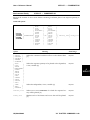
The PostScript Plot Program
The program nastplotps reads both binary and formatted plot files generated by UAI/NASTRAN
and generates an Encapsulated PostScript file. This PostScript output can then be either sent to a
printer or imported into a text formatting program which accepts Encapsulated PostScript input.
Importing the plot only makes sense when the plot file contains a single frame or if you use the -pn
option to explicitly create a single plot. The program allows you to select fonts, control paper size
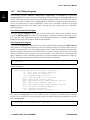
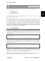
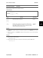
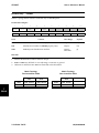
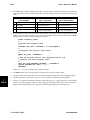
and to determine output orientation (landscape or portrait). Detailed documentation on these options is available by executing the following command with no arguments:
nastplotps
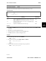
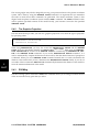
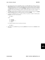
The on-line help is:
Usage: nastplotps options file_name_1 file_name_2 ...
-b = plot files are binary (default)
-f = plot files are formatted
-nf = suppress frame around plot
-pn# = only plot number # is processed
-pw# = paper width (default -pw8.5)
-mw# = unplottable margin width (default -mw0.25)
-ph# = paper height (default -ph11.0)
-mh# = unplottable margin height (default -mh0.25)
-por = portrait orientation (default)
-lan = landscape orientation
-tx = typeface (default -tHelvetica)
The output of nastplotps is to Unix standard output. Normally, you should redirect standard
output to a file or pipe it to a print spooling program as desired. The following illustrates a typical
use of nastplotps:
nastplotps -f -lan mydata.plt | lpr -Pps
1-10 EXECUTING THE PROGRAM
UAI/NASTRAN
User’s Reference Manual
The HP-GL Plot Program
The program nastplotgl reads both binary and formatted plot files generated by UAI/NASTRAN
and generates HP-GL commands. This HP-GL output can then be either sent to a printer or plotter.
It may also be imported into a text formatting program which accepts GL input. Importing the plot
only makes sense when the plot file contains a single frame or if you use the -pn option to
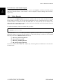
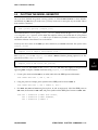
explicitly create a single plot. Detailed documentation on the plotter options is available by executing the following command with no arguments:
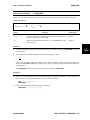
nastplotgl
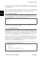
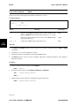
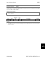
The on-line help is:
Usage: nastplotgl options file_name_1 file_name_2 ...
-b = plot files are binary (default)
-f = plot files are formatted
-nf = suppress frame around plot
-pn# = only plot number # is processed
-pw# = paper width (default -pw8.5)
-mw# = unplottable margin width (default -mw0.25)
-ph# = paper height (default -ph11.0)
-mh# = unplottable margin height (default -mh0.25)
The output of nastplotgl is to Unix standard output. Normally, you should redirect standard
output to a file or pipe it to a print spooling program as desired.
The X-Window, Motif Interface Plot Program
For computer systems which support the X-Window system, the plotting program nastplot is
provided. This program, which operates in the X-Window environment, uses a Motif interactive
interface. nastplot provides the following functional capability for viewing and processing
UAI/NASTRAN plot files:
❒
Automatic recognition and processing of binary or formatted plot files.
❒
Full support of the LINESTYLE command using user selectable display colors.
❒
Direct selection of display for any plot in the plot file.
❒
Zooming of the plot display.
❒
Export of plots to either a printer or a file, using either PostScript or HP-PCL display
languages.
nastplot is executed with the command:
nastplot [ file_name ]
Detailed online help is provided by the nastplot program.
UAI/NASTRAN
EXECUTING THE PROGRAM 1-11
1
JCL
User’s Reference Manual
Special Versions of the nastplot Program
1
JCL
On HP/Apollo and Sun workstations special versions of nastplot are delivered which operate
under the normal window system found on those computers, Display Manager and SunView,
respectively.
1.2.8
Online Manuals
The entire suite of UAI/NASTRAN manuals is available online in the Adobe Portable Document
Format (PDF). This allows you to view the documentation on any computer that has the Adobe®
Acrobat® Reader 3.0. Readers for DEC, HP, IBM, MAC, PC, SGI, and Sun (OS and Solaris) were
delivered with your system. Any other readers that become available can be downloaded from the
Adobe Web site at www.adobe.com.
To use the documents, from the command line you enter:
uaidoc [manual_name]
If you omit the manual_name, then you will see a splash screen that allows you to navigate to the
appropriate manual. You may also go directly to a manual by placing its name on the command
lines. The names of the UAI/NASTRAN manuals are:
❒
Nastran_Reference_Manual
❒
Nastran_Users_Guide
❒
Nastran_Schemata_Manual
❒
UAI_Unix_Support_Manual
Check the UAI Web site at www.uai.com for any interim updates and additions to the electronic
documentation.
1-12 EXECUTING THE PROGRAM
UAI/NASTRAN
User’s Reference Manual
1.3
DEC VAX SERIES COMPUTERS — VMS OPERATING SYSTEM
This section describes the host-dependent information that you need to execute UAI/NASTRAN on
DEC VAX computers under the VMS operating system.
1.3.1
Executing UAI/NASTRAN
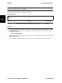
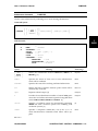
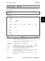
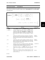
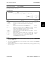
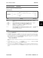
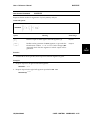
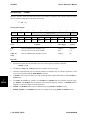
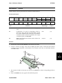
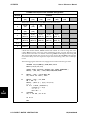
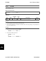
A command procedure, called NASTRAN, is provided to execute the program. To execute you enter:
NASTRAN
filename
[/WSL=n][/AFT=time] /PRT=
JID=filename
NO
YES
−
[/SPREF=pref_file][/UPREF=pref_file][/LPREF=pref_file]
[/T=cpu_time][/QUE=queuename]
where:
filename
Specifies the file name that contains the UAI/NASTRAN input data stream.
The actual file specifications must have a type of .DAT. If you omit the
filename, you will be prompted for it.
n
Specifies the working set size limit for the run.
time
Specifies the time-of-day at which the UAI/NASTRAN execution will begin.
The general form of time is:
dd-mmm-yyyy:hh:mm:ss.ss
Refer to your VAX/VMS DCL Dictionary Manual for a complete description
of the format.
NO
YES
Requests that the output and log files be saved or printed and deleted. If the
default value, NO, is selected, then the files filename.PRT and
filename.LOG will be saved in your directory. If you select YES, then both
files will be printed on your line printer and then deleted.
pref_file
Preference file substitution strings.
cpu_time
Specifies the CPU time limit for the execution in the form:
hh:mm:ss
queuename
Specifies the name of the batch queue into which the job will be placed.
The pref_file specifies the substitution string used to generate Preference File names. You may
specify a different string for the system (SPREF), the user (UPREF) and the local (LPREF) preference
files. If you have the unusual case where all of these files have the same name, you may use the
option PREF followed by the pref_file. This procedure submits a batch job which executes
UAI/NASTRAN using the specified filename. Some of the results of this execution may create
UAI/NASTRAN
EXECUTING THE PROGRAM 1-13
1
JCL
User’s Reference Manual
1
JCL
output files. These are described in the next section. The keyword parameters used by the procedure may be specified in any order, but they must be separated by the slash character, "/", a
comma, or a blank. Consider the following examples:
1.
Execute UAI/NASTRAN for the input data stream contained in file TEST.DAT:
NASTRAN TEST
2.
Submit a batch job that will execute UAI/NASTRAN using the file TEST.DAT after 10:00 PM and
request that the output print file be printed and then deleted.
NASTRAN TEST/AFT=22:00:00/PRT=YES
1.3.2
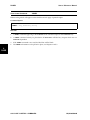
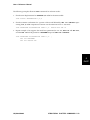
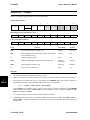
UAI/NASTRAN File Names
When you execute the NASTRAN script a number of files may be created which have names that are
automatically generated by the program. These are described in this section.
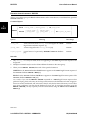
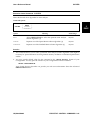
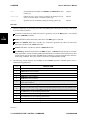
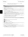
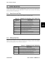
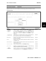
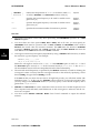
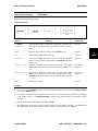
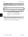
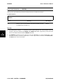
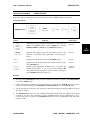
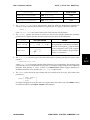
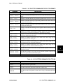
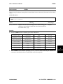
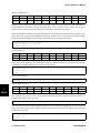
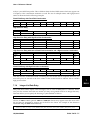
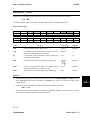
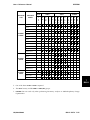
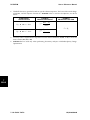
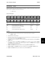
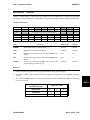
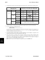
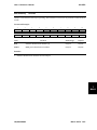
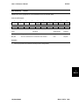
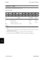
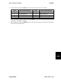
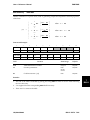
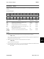
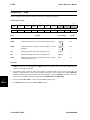
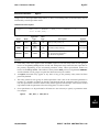
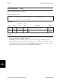
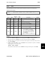
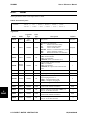
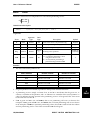
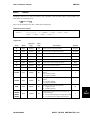
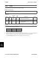
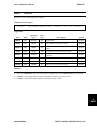
Unique UAI/NASTRAN files
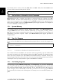
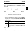
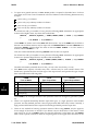
There are four unique files that are used frequently by UAI/NASTRAN. These are unique in the
sense the program will automatically define file names for these if you do not explicitly ASSIGN
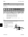
them. These files, and their default names, are shown in the table below:
FILE
May Override with
ASSIGN Command?
Generated Name if ASSIGN
Command is Not Used
The print file
NO
filename.PRT
The UAI log file
NO
filename.SUM
The BULK file
YES
filename.BULK
The PUNCH file
YES
filename.PCH
The filename represents the name of the file containing the UAI/NASTRAN input data stream.
The UAI log file is a special file that contains the history of your execution. Upon completion of the
job, the log file is appended to the print file, and then deleted. VMS jobs also generate a log file
which is named filename.LOG. Depending on the options specified at your site, this file may also
contain information similar to that found in the UAI log file.
Databases
You will recall from Section 1.1.4 that each database that you use during an execution is comprised
of at least two physical files. The trailing components of these file names is always generated by
UAI/NASTRAN. When you ASSIGN a database with a status of NEW and provide a physical file
name, phys_name, the program generates the file names:
phys_name.EDB and phys_name.DF000
1-14 EXECUTING THE PROGRAM
UAI/NASTRAN
User’s Reference Manual
There may be times, most often in the case of the RUNDB, that you ASSIGN a database with a status
of TEMP. In such cases, the program internally generates file names that are unique to your job. The
detailed rules used to generate these names are given in the System Support Manual. These simple
rules pertain to the simplest and most used ASSIGNments of databases. If you are using very large
databases, then there are additional rules. These will be provided by your UAI/NASTRAN System
Support Specialist.
1.3.3
Monitoring the Execution
There are two ways that you may monitor the progress of your batch job. The process name field of
the VMS command
SHOW SYSTEM/BATCH
will display the filename being executed and the UAI/NASTRAN module that is currently being
executed. If allowed by your UAI/NASTRAN System Support Specialist, you may also examine the
batch log file which provides a history of the UAI/NASTRAN modules as they execute.
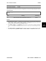
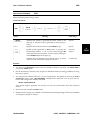
1.3.4
ASSIGN and INCLUDE Command Parameters
There are no additional parameters to the INCLUDE command for VAX/VMS host computers.
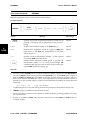
The ASSIGN Executive Control command has several parameters. The NEWVER parameter complements the REALLOC parameter in controlling the manner in which UAI/NASTRAN handles duplicate file when the ASSIGN command has a disposition of NEW. The REALLOC option causes the
latest version of the existing file to be deleted and reallocated by the job. The NEWVER option, on the
other hand, causes the existing version to be kept and a new version created. If you do not specify
one of these options, your job will fail if a specified file already exists. Two other special parameters, ILOC and DLOC, are used to control the location of the physical files comprising a database.
Contact your UAI/NASTRAN System Support Specialist for a complete description of how these
parameters are used.
Examples of ASSIGN commands are given below:
1.
Assign a file in your UAI/NASTRAN data stream which has the file name DB1:[A]WING.OP2.
Assume the file, which is new, will be used to export data using the OUTPUT2 module and you
wish to use the logical name OP2 for the file.
ASSIGN OP2=DB1:[A]WING.OP2,NEW,USE=OUTPUT2,REALLOC
2.
Perform the same operation as above, but assume that you are saving different OUTPUT2 results
as different versions of the same file. Then the following ASSIGN command is used:
ASSIGN OP2=DB1:[A]WING.OP2,NEW,USE=OUTPUT2,NEWVER
UAI/NASTRAN
EXECUTING THE PROGRAM 1-15
1
JCL
User’s Reference Manual
If you already had two versions of this file, WING.OP2;1 and WING.OP2;2, then the OUTPUT2 results
from the current execution will be placed in the file:
1
JCL
WING.OP2;3
1.3.5
Site Definition of Automatic ASSIGN Commands
UAI/NASTRAN provides a capability which allows an individual client site to define a set of ASSIGN commands which are used automatically by the program as needed. When this feature is
used, it is not necessary for you to specify your own ASSIGN commands if the appropriate automatic ones are available. Contact your UAI/NASTRAN System Support Specialist for a complete list
of automatic ASSIGNs available at your site.
1.3.6
Dynamic Memory
You generally define the amount of dynamic memory to be used by your UAI/NASTRAN job by
using the MEMORY Executive Control command. Additionally, you may specify a working set limit,
WSL, when you invoke the command procedure. This is an advanced feature that may impact the
performance of your host computer. Contact your UAI/NASTRAN System Support Specialist for
complete details.
1.3.7
The eShell Program
If your site has the eShell interactive eBase interface program, then to execute this program you
enter:
eshell [ database ]
where:
database
Is the name of a database to be opened with read access.
This command will execute eShell in the interactive mode and, optionally, open the database that
you specify with read access. Unless directed otherwise by eShell commands, all subsequent output
will be sent to the terminal device. The eShell Tutorial Problem library is available. Contact your
Systems Support Specialist to obtain the name of the directory where these problems may be found.
A description of how you may use them is given in the eShell User’s Manual.
1.3.8
The Plotting Programs
Three plotting programs, TEKPLOT, nastplotps, and nastplotgl, are provided. nastplotps
may be used to create files using the PostScript language, and nastplotgl may be used to create
files using the Hewlett-Packard graphics language, HP-GL. These files may then be routed to a
printer or display device. Additionally, source code is provided in the form of program TEKPLOT
which provides your facility with a starting point for creating your own customized plotting program.
1-16 EXECUTING THE PROGRAM
UAI/NASTRAN
User’s Reference Manual
The Tektronix PLOT10 Plot Program
A Fortran program, TEKPLOT, is provided in source code format, which you may modify and use
to process UAI/NASTRAN plot files and create displays on graphics terminals connected to your
host computer which support the Tektronix PLOT10 graphics instructions. Contact your UAI/NASTRAN System Support Specialist for additional information.
The PostScript Plot Program
The program NASTPLOTPS reads both binary and formatted plot files generated by UAI/NASTRAN
and generates an Encapsulated PostScript file. This PostScript output can then be either sent to a
printer or imported into a text formatting program which accepts Encapsulated PostScript input.
Importing the plot only makes sense when the plot file contains a single frame or if you use the /PN
option to explicitly create a single plot. The program allows you to select fonts, control paper size
and to determine output orientation (landscape or portrait).
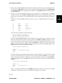
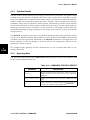
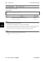
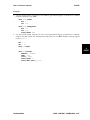
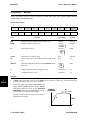
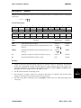
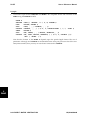
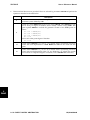
A command procedure called NASTPLOTPS is provided to allow you to create these PostScript files.
To execute, you enter:
NASTPLOTPS /TYPE = BINARY
FORMAT
/ORIENT = PORTRAIT
LANDSCAPE
[ /NOFRAME ]
[/PN = #][/PW = #][/MW = #][/PH = #][/MH = #]
[TYPEFACE=tf][/OUTPUT=filename] plotfile_1 plotfile_2
…
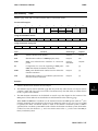
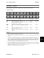
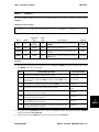
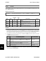
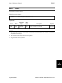
where:
BINARY
FORMAT
PORTRAIT
LANDSCAPE
Specifies the plot file format. The default is BINARY.
Specifies the paper orientation. The default is PORTRAIT.
/NOFRAME
Suppresses the frame around the plot.
/PN=#
Processes single plot with sequence number #.
/PW=#
Sets paper width. The default is 8.5 in.
/MW=#
Specifies unplottable margin width. Default 0.25 in.
/PH=#
Specifies paper height. The default 11.0 in.
/MH=#
Specifies unplottable margin height. The default 0.25 in.
/TYPEFACE=tf]
Selects a PostScript typeface. The default is Helvetica.
/OUTPUT=filename Specifies the file name which will contain the resulting Encapsulated
PostScript file. If omitted, output is routed to SYS$OUTPUT.
plotfile_i
UAI/NASTRAN
Specifies the file names which contains your plot files created by a
UAI/NASTRAN job.
EXECUTING THE PROGRAM 1-17
1
JCL
User’s Reference Manual
1
JCL
Normally you should redirect SYS$OUTPUT to a file. This file may then be routed to the PostScript
printer, if available, at your facility.
The HP-GL Plot Program
The program NASTPLOTGL reads both binary and formatted plot files generated by UAI/NASTRAN
and generates HP-GL commands. This HP-GL output can then be either sent to a printer or plotter.
It may also be imported into a text formatting program which accepts GL input. Importing the plot
only makes sense when the plot file contains a single frame or if you use the /PN option to
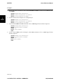
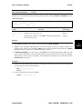
explicitly create a single plot. A command procedure called NASTPLOTGL is provided to allow you
to create these files. To execute, you enter:
NASTPLOTGL
/TYPE = BINARY
FORMAT
[ /NOFRAME ] [/PN = #][/PW = #]
[/MW = #][/PH = #][/MH = #] [/OUTPUT=filename ]
plotfile_1
plotfile_2 …
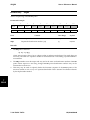
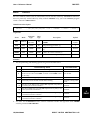
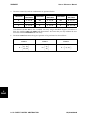
where:
BINARY
FORMAT
Specifies the plot file format. The default is BINARY.
/NOFRAME
Suppresses the frame around the plot.
/PN=#
Processes single plot with sequence number #.
/PW=#
Sets paper width. The default is 8.5 in.
/MW=#
Specifies unplottable margin width. The default 0.25 in.
/PH=#
Specifies paper height. The default 11.0 in.
/MH=#
Specifies unplottable margin height. The default 0.25 in.
/OUTPUT=
filename
Specifies the file name which will contain the resulting Encapsulated
PostScript file. If omitted, output is routed to SYS$OUTPUT.
plotfile_i
Specifies the file names which contains your plot files created by a
UAI/NASTRAN job.
Normally you should redirect SYS$OUTPUT to a file. This file may then be routed to the PostScript
printer, if available, at your facility.
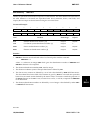
1.3.9
Online Manuals
The entire suite of UAI/NASTRAN manuals is available online in the Adobe Portable Document
Format (PDF). This allows you to view the documentation on any computer that has the Adobe®
Acrobat® Reader 3.0. Readers for DEC, HP, IBM, MAC, PC, SGI, and Sun (OS and Solaris) were
delivered with your system. Any other readers that become available can be downloaded from the
Adobe Web site at www.adobe.com.
1-18 EXECUTING THE PROGRAM
UAI/NASTRAN
User’s Reference Manual
To use the documents, from the command line you enter:
1
JCL
uaidoc [manual_name]
If you omit the manual_name, then you will see a splash screen that allows you to navigate to the
appropriate manual. You may also go directly to a manual by placing its name on the command
lines. The names of the UAI/NASTRAN manuals are:
❒
Nastran_Reference_Manual
❒
Nastran_Users_Guide
❒
Nastran_Schemata_Manual
❒
UAI_VMS_Support_Manual
Check the UAI Web site at www.uai.com for any interim updates and additions to the electronic
documentation.
UAI/NASTRAN
EXECUTING THE PROGRAM 1-19
User’s Reference Manual
1
JCL
This page is intentionally blank.
1-20 EXECUTING THE PROGRAM
UAI/NASTRAN
User’s Reference Manual
2
EXEC
Chapter 2
EXECUTIVE CONTROL COMMANDS
Executive Control commands provide UAI/NASTRAN with general information describing the analysis to be performed. The Executive Control command packet is the first in the input data stream as
shown in Figure 2-1.
Figure 2-1. EXECUTIVE CONTROL PACKET LOCATION
EXECUTIVE
CONTROL
COMMANDS
SUBSTRUCTURE
COMMANDS
CASE CONTROL
COMMANDS
BULK DATA
ENTRIES
In addition to Executive Control commands, this data packet may contain one or more subpackets
that are used to modify Rigid Formats, to restart a previous analysis or to create a specialized DMAP
program.
Rev: Ver20.1
UAI/NASTRAN
EXECUTIVE CONTROL COMMANDS 2-1
User’s Reference Manual
2.1
THE EXECUTIVE CONTROL COMMANDS
The general form of the Executive Control command packet is:
command option_list
command option_list
...
[RESTART Subpacket]
[ALTER Subpacket] or [DMAP Subpacket]
CEND
2
EXEC
The packet contains a number of commands, most of which have an additional option_list.
Three optional subpackets may also be present. These are the DMAP Subpacket, the RESTART
Subpacket, and the ALTER Subpacket, all of which are described in this chapter. The available
commands are summarized in Table 2-1.
Table 2-1. SUMMARY OF EXECUTIVE CONTROL COMMANDS
COMMAND
DESCRIPTION
$
Indicates a comment entry.
ALTER
Edits a Rigid Format DMAP sequence.
APPROACH
Selects the analysis approach or discipline.
ASSIGN
Assigns physical file names.
BEGIN
Defines the start of a DMAP sequence.
CEND
Indicates the end of the Executive Control packet.
CHKPNT
Selects the CHECKPOINT option.
DATACHECK
Enables specific data checking features.
DIAG
Selects diagnostic output.
ECHOON and ECHOOFF
Enables and disables the echoing of Executive Control commands.
END
Defines the end of a DMAP sequence subpacket
ENDALTER
Defines the end of a Rigid Format ALTER packet.
ID
Defines the start of the Executive Control packet.
IMPORT
Imports a Rasna Appled Structure model.
INCLUDE
Inserts the contents of an external file into the input data stream.
LINES
Specifies the number of printed lines on a page.
MAXLINES
Limits the total number of lines of print.
MEMORY
Specifies the amout of memory UAI/NASTRAN will use.
PRINT CONFIGURATION
Requests a printed echo of your current Configuration.
SEQUENCE
Controls the GRID point sequencer.
SKIPON and SKIPPOFF
Disables or enables the processing of Executive Control commands.
SOLUTION
Selects a Rigid Format.
SOLVER
Controls the use of the Sparse Matrix Solver for static analysis.
TIME
Specifies the maximum allowable execution time.
2-2 EXECUTIVE CONTROL COMMANDS
UAI/NASTRAN
User’s Reference Manual
2.2
EXECUTIVE CONTROL SUBPACKETS
There are three optional subpackets that may be included in the Executive Control packet:
❒
The ALTER Subpacket
❒
The DMAP Subpacket
❒
The RESTART Subpacket
2
EXEC
Each of these is described below and examples of their use are given. However, first a word about
some nomenclature in this manual.
Note that UAI/NASTRAN creates an output file, called the Print File, which is formatted and suitable
for routing to a standard, 132 character wide printer. At most installations, this file is not automatically routed to the printer. You may review the contents of this file using your standard text editor,
and then dispose of the file as you wish. Thus, the generation of output for this file is often referred
to as a Print Operation. Also, an alternate form of output is available which once requested the
generation of physical punched computer cards. Today, however, this output is written to a logical
file that you have assigned with the option USE=PUNCH. This file is always formatted in 80 byte
records and it may also be examined with a text editor.
2.2.1
The ALTER Subpacket
To modify a standard Rigid Format, for instance to print some intermediate results, an ALTER
subpacket is used. The ALTER commands allow the deletion or insertion of new DMAP statements
into the Rigid Format. For example, to print the stiffness matrix used for a static analysis, an ALTER
subpacket might be:
ALTER 20
MATPRN KAA,,,,// $
ENDALTER
This subpacket may appear anywhere within the Executive Control packet. The ALTER subpacket
always begins with an initial ALTER command. As many ALTER commands may be used as desired, but the DMAP statement numbers must appear in increasing sequence number. The ALTER
commands are of the form:
ALTER i
or
ALTER j,k
In the first case, i is a DMAP statement number and the following DMAP statements will be inserted
after statement i. In the second case, existing Rigid Format statements numbered j through k will
be replaced by the DMAP statements which follow the ALTER command.
Note that only one ALTER subpacket may appear in the Executive Control packet. This means that
ALTER commands may not be interspersed with other Executive Control commands.
UAI/NASTRAN
EXECUTIVE CONTROL COMMANDS 2-3
User’s Reference Manual
The ALTER subpacket may be terminated by either an ENDALTER command or the CEND command.
Thus, the ALTER subpacket is often placed at the end of the Executive Control packet and CEND is
used as the terminator.
Chapter 8 contains documentation for DMAP statements which may be used in the ALTER subpacket. To get the DMAP listings for the Rigid Formats you use the Executive Control command
DIAG,14. Finally, note that the MULTI Solution Sequence may not be modified by the user.
2
EXEC
2.2.2
The DMAP Subpacket
To use the Direct Matrix Abstraction Program (DMAP) feature of UAI/NASTRAN, detailed in Chapter 8, the APP DMAP Executive Control command is selected. A DMAP subpacket is then entered
into the Executive Control packet. This subpacket must have the form:
BEGIN $
...
...
...
END $
This subpacket must also appear prior to the CEND command. Only one DMAP subpacket may be
included in the Executive Control command packet.
2.2.3
The RESTART Subpacket
The RESTART subpacket consists of commands which are automatically generated by a previous
UAI/NASTRAN execution in which a checkpoint operation was requested. The CHECKPOINT execution created these commands and stored them on the UAI/NASTRAN logical file which is assigned
with USE=DICT. These commands are a table of contents of the RESTART File, which is a logical file
that you have assigned with USE=CHKPNT, which was also created in this previous execution.
To perform a RESTART using your previous CHECKPOINT results, the RESTART subpacket must be
inserted into the Executive Control packet along with an ASSIGN command for the RESTART File.
The RESTART File, which is the same physical file that you used for the CHECKPOINT, is now
assigned with the option USE=RESTART. The RESTART subpacket is normally inserted into the
Executive Control packet by using the INCLUDE command.
An example of the proper use of these commands is shown next. First, the following Executive
Control commands perform the CHECKPOINT operation:
ID CHECKPOINT,RUN
APP DISP
SOL 1
CHKPNT YES
ASSIGN DICT=DICT.DAT,NEW,USE=DICT
ASSIGN NPTP=RESTARTFILE,NEW,USE=CHKPNT
CEND
Then these commands perform the RESTART operation:
2-4 EXECUTIVE CONTROL COMMANDS
UAI/NASTRAN
User’s Reference Manual
ID RESTART,RUN
APP DISP
SOL 1
ASSIGN OPTP=RESTARTFILE,OLD,USE=RESTART
INCLUDE DICT.DAT
CEND
Note that the status of the RESTART File is OLD, indicating that it already exists. Also note that the
MULTI Solution Sequence may not be restarted.
2.2.4
Configuration Parameters
As indicated in Chapter 1, UAI/NASTRAN is configured to perform optimally on a given host computer. This is done by using Configuration Files. Some of the items in the [UAI/NASTRAN] Component of the Configuration File control parameters are found in Executive Control commands. When
this is the case, the item is noted for the specific command.
UAI/NASTRAN
EXECUTIVE CONTROL COMMANDS 2-5
2
EXEC
User’s Reference Manual
2.3
EXECUTIVE CONTROL COMMAND DESCRIPTIONS
Executive Control commands are free-field entries. In presenting the general syntax of each command and its options, the following conventions are used:
❒
Many Executive Control commands contain keywords. All keywords are shown in capitalized, bold computer type such as: ALTERLIB. All such keywords must be entered exactly
as they are specified, subject only to the exception that they may be abbreviated by their first
four characters.
❒
Some commands contain parentheses. These must be entered if an option requiring them is
selected.
❒
Lower case italicized computer type, such as altername, indicates that you must provide
a specific data value.
❒
Braces { } enclose a list of two or more options from which you may select one.
❒
Brackets [ ] indicate that the enclosed keywords and parameters may be omitted when you
use the command.
❒
When a choice is to be made from a list, the default choice is presented in boldface type as
CHOICE1
in the following: CHOICE2
DEFAULT
A single command line may not exceed 72 characters. However, you may continue a
command by ending the current record with a comma and continuing to the next record.
2
EXEC
❒
Additionally, command options have a valid data range and, in some cases, a default value. The
following table defines the data range specifications found in this chapter.
DATA
RANGE
SPECIFIER
MEANING
Integer
The data must be an integer number in the range of indicated
values.
Real
The data must be a real number in the range of indicated
values.
Character
The data must be a string of characters beginning with a letter.
Keyword
The data must be a character string matching the first four or
more unique characters of a keyword option.
2-6 EXECUTIVE CONTROL COMMANDS
UAI/NASTRAN
$
User’s Reference Manual
Executive Control Command
$
[ Comment ]
[ Comment ]
Defines the beginning of commentary text.
Command Syntax:
$ any_character_string
2
EXEC
Examples:
1.
Enter a comment line in the Executive Control packet:
APP DISP
$ EXECUTE A STATICS ANALYSIS
SOL 1
2.
Place a comment after an Executive Control command:
TIME = 10 $ SPECIFY A TIME LIMIT RATHER THAN USE THE DEFAULT VALUE
UAI/NASTRAN
EXECUTIVE CONTROL COMMANDS 2-7
ALTER
User’s Reference Manual
Executive Control Command
ALTER
Modifies the Direct Matrix Abstraction Program (DMAP) sequence of a Rigid Format.
Command Syntax:
ALTER line1
2
EXEC
[ , line2 ]
Option
Meaning
Data Range
line1
Specifies a DMAP instruction statement number which, if
line2 is absent, defines a statement after which the ensuing
DMAP commands are entered.
Integer>0
line2
Specifies a second DMAP statement number which, with
line1, defines a range of instructions to be deleted and replaced by any following DMAP instructions.
Integer>0
line2≥line1
Remarks:
1.
Successive ALTER commands must reference statement numbers which are in increasing order.
2.
The ALTER subpacket is terminated by either an ENDALTER or CEND command.
Examples:
1.
Insert DMAP statements after line 22:
ALTER 22
...
2.
Delete line 5 of the selected Rigid Format:
3.
Replace lines 38 through 45 with one or more new DMAP statements.
ALTER 5,5
ALTER 38,45
...
2-8 EXECUTIVE CONTROL COMMANDS
UAI/NASTRAN
APPROACH
User’s Reference Manual
Executive Control Command
APPROACH
Selects the analytical approach for the UAI/NASTRAN execution.
Command Syntax:
APP
DISPLACEMENT
NONLINEAR
HEAT
DMAP
Option
2
EXEC
Meaning
Data Range
DISPLACEMENT
Specifies that one of the Linear Structural Analysis Rigid Formats, or the Multidisciplinary Solution sequence, will be
used.
Keyword
NONLINEAR
Specifies that a Nonlinear Structural Analysis Rigid Format
will be used.
Keyword
HEAT
Specifies that one of the Heat Transfer Rigid Formats will be
used.
Keyword
DMAP
Specifies that a Direct Matrix Abstraction Program (DMAP)
will be provided by the user.
Keyword
Remarks:
1.
The following table summarizes the APP command that is used in performing different types of
analyses with UAI/NASTRAN:
ANALYSIS TYPE
APP COMMAND
NOTE
Linear Structural Analysis Rigid Formats
and Multidisciplinary Solution Sequence
APP DISP
Optional
Nonlinear Structural Analysis Rigid Formats
APP NONLINEAR
Required
Heat Transfer Rigid Formats
APP HEAT
Required
User-written DMAP program
APP DMAP
Required
User-written ALTERs that replace the automatically
generated Substructuring DMAP Solutions [2]
APP DISP,SUBS,1
Required [3]
2.
See Chapter 19 of the User’s Guide for examples of using ALTERs with the Substructuring capability.
3.
This form is only necessary if there is a conflict between your ALTERs and the Substructuring
ALTERs. If this is the case, the command is used to remove all of the automatically generated
ALTERs. As a result, you must provide all of the DMAP.
Rev: V20.1
UAI/NASTRAN
EXECUTIVE CONTROL COMMANDS 2-9
ASSIGN
User’s Reference Manual
Executive Control Command
ASSIGN
Selects UAI/NASTRAN data files prior to execution.
Command Syntax:
2
EXEC
For Databases:
NEW
ASSIGN logical_name [= phys_name] , OLD [,USE=use][,REALLOC]
TEMP
[,PASSWORD = pass][,IBLKSIZE = nwib][,DBLKSIZE = nwdb]
READ
,ACCESS = WRITE [,params]
ADMIN
For Other Files:
NEW
ASSIGN logical_name [= phys_name] , OLD
TEMP
[,USE = use][,REALLOC]
TYPE = , BINARY [,BLKSIZE = nwblk][,params]
FORMATTED
Option
Meaning
Data Range
logical_name
Defines a logical UAI/NASTRAN file name. [1]
Character
phys_name
Is the operating system dependent physical file name that
you wish assigned to the logical_name file. If not provided, then logical_name is used.
[2]
NEW
OLD
TEMP
Defines the status of the file. The file may be NEW, in which
case it is allocated at run-time, an existing or OLD file, which
is the default, or a TEMP file which is deleted at the end of the
run. [3]
Keyword
use
Defines how the assigned file will be used. If not provided,
then logical_name is used.
[4]
REALLOC
Requests that a new physical file be reallocated if it already
exists. [5]
Keyword
pass
Specifies the database password. [6]
Character
2-10 EXECUTIVE CONTROL COMMANDS
UAI/NASTRAN
ASSIGN
User’s Reference Manual
nwib
Index file blocksize, in words. Used for databases only. [7]
Integer>0
nwdb
Data file blocksize, in words. Used for databases only. [7]
Integer>0
READ
WRITE
ADMIN
Specifies the type of access that will be allowed for a database with a status of OLD. [6]
Character
params
Host computer dependent parameters.
[10]
Specifies the type of output that will be written on the file.
[8,9]
Character
Sequential file blocksize, in words. [7]
Integer>0
BINARY
FORMATTED
nwblk
Remarks:
1.
The ASSIGN command is optional, it overrides any default assignments made in the <Assign
Processing> group of the [UAI/NASTRAN] Configuration Section. You may use the command:
PRINT CONFIGURATION
to obtain the defaults. Your System Support Specialist can provide you with more information
about this advanced UAI/NASTRAN feature.
2.
The logical file name logical_name is used in DMAP instructions which you use to create files
that will be exported from, or imported into, UAI/NASTRAN, and it is also used directly in certain
other commands. Otherwise it may be one of the use names, removing the need for the specification of the use parameter. See the examples below.
2.
Physical file names vary depending on your host computer. See Chapter 1 for details.
3.
Additional options may be available for different host computers. See Chapter 1.
4.
The table below summarizes the available UAI/NASTRAN file uses:
USE
FILE CONTAINS OR WILL
CONTAIN:
USED WHEN:
ARCHIVE
ARCHIVE Database
When requesting data archival with the
ARCHIVE Case Control command.
BULK
Bulk Data PUNCH requests
Any Bulk Data PUNCH requests are made.
CHKPNT
CHECKPOINT information
Performing a CHECKPOINT execution.
DICT
The CHECKPOINT dictionary
Performing a CHECKPOINT execution.
IMPORT
UAI/NASTRAN ARCHIVE Database Importing an existing model.
INPUTT1
INPUTT2
INPUTT3
INPUTT4
INPUTT5
UAI/NASTRAN Import File
NLDB
Nonlinear Database
OUTPUT1
OUTPUT2
OUTPUT4
OUTPUT5
UAI/NASTRAN Export File
UAI/NASTRAN
Reading files that were created in earlier
UAI/NASTRAN jobs by using modules OUTPUT1,
OUTPUT2, OUTPUT4 or OUTPUT5, or were created
by an external FORTRAN program.
Performing Nonlinear Analyses.
Writing files using modules OUTPUT1, OUTPUT2,
OUTPUT4, or OUTPUT5.
EXECUTIVE CONTROL COMMANDS 2-11
2
EXEC
ASSIGN
USE
2
EXEC
User’s Reference Manual
FILE CONTAINS OR WILL
CONTAIN:
USED WHEN:
PLOT
UAI/NASTRAN plot directives
OUTPUT(PLOT), OUTPUT(XYPLOT), or Substructuring PLOT commands are present.
PUNCH
Data for which PUNCH is requested
Any PUNCH requests are made for any solution
results.
RESTART
RESTART information
RESTARTing a previous job. You must also
INCLUDE the DICT file from the CHECKPOINT run.
RUNDB
Run-time Database
Running any UAI/NASTRAN job.
SOF
Substructure Database
Performing Substructuring Analyses.
SOFIN
Substructure Database
Importing an SOF Substructure database that
was previously exported with module SOFOUT.
SOFOUT
Substructure Database
Exporting the SOF Substructure database.
5.
If you specify NEW for a file that already exists, and you do not include the REALLOC parameter,
your job will be terminated.
6.
Passwords are used, but they are not required, only when USE is RUNDB, ARCHIVE, SOF or
NLDB. For databases with a STATUS of NEW, the same password is used for the READ, WRITE and
ADMIN privileges. The eShell command:
SET PASSWORD
may be used to change any or all of the passwords as desired. For OLD databases, the password
must match the access type specified by the ACCESS parameter.
7.
You may provide default value for this command in the <Computing Resources> group of the
[eBase:applib] Section of your Configuration.
8.
This parameter is only needed when the file USE is PLOT, INPUTT4, INPUTT5, OUTPUT4, OUTPUT5, SOFIN, and SOFOUT.
9.
When a BINARY type is specified, you may combine output from modules OUTPUT2 and OUTPUT4 on the same file.
10. Other host computer dependent parameters may be available. See Chapter 1 for details.
Examples:
1.
Any of the following ASSIGN commands may be used to define a new OUTPUT2 file to be saved
for post-processing:
ASSIGN USER1=MYFILE,NEW,USE=OUTPUT2,REALLOC
ASSIGN OUTPUT2=MYFILE,NEW,REALLOC
ASSIGN OUTPUT2=MYFILE,NEW,USE=OUTPUT2,REALLOC
ASSIGN MYFILE,NEW,USE=OUTPUT2,REALLOC
2.
You may use any of the following commands to create a new Substructure Database:
ASSIGN SOF=MYSOF,NEW,REALLOC
ASSIGN MYSOF,NEW,USE=SOF,REALLOC
2-12 EXECUTIVE CONTROL COMMANDS
UAI/NASTRAN
BEGIN
User’s Reference Manual
Executive Control Command
BEGIN
Defines the beginning of a DMAP Subpacket and selects compiler options.
Command Syntax:
BEGIN
GO
NOGO
, ERR = level ,
NOLIST
LIST
,
Option
,
NOREF
REF
NODECK
DECK
,
Meaning
NOWARN
WARN
2
EXEC
$
Data Range
Requests DMAP program compilation and execution, or termination of UAI/NASTRAN after compilation.
Keyword
ERR=level
Defines the error level at which suspension of execution
will occur. level=0 selects the warning error level,
level=1 the potentially fatal error level, and a level=2 the
fatal error level. [1]
0≤Integer≤2
Default=2
LIST
NOLIST
Selects or deselects DMAP program listing option.
Keyword
DECK
NODECK
Selects or deselects writing the DMAP program to the PUNCH
file. [2]
Keyword
REF
NOREF
Selects or deselects creating a DMAP cross-reference listing.
Keyword
WARN
NOWARN
Selects or deselects warning message print. If WARN is selected, then warning and potentially fatal error messages are
printed, otherwise they are not. [1]
Keyword
GO
NOGO
Remarks:
1.
If you ALTER a Rigid Format, then the NOWARN default is changed to WARN.
2.
You must use the ASSIGN Executive Control command to define a logical file with USE=PUNCH if
you use the DECK option.
3.
All Rigid Formats start with a BEGIN command. To request other than the default compiler
options, you replace the BEGIN command. For example:
ALTER 1,1
BEGIN NOGO, REF $
UAI/NASTRAN
EXECUTIVE CONTROL COMMANDS 2-13
CEND
Executive Control Command
User’s Reference Manual
CEND
Defines the end of the Executive Control command packet.
Command Syntax:
CEND
2
EXEC
Remarks:
1.
This command is mandatory and must be the last input record in the Executive Control command
packet.
2-14 EXECUTIVE CONTROL COMMANDS
UAI/NASTRAN
CHKPNT
User’s Reference Manual
Executive Control Command
CHKPNT
Requests the creation of a CHECKPOINT file which can be used later during a RESTART execution.
Command Syntax:
CHKPNT
YES
NO
2
EXEC
Remarks:
1.
Unless defaults are provided in your Configuration, you must use the ASSIGN Executive Control
command to define two logical files, one with USE=DICT and one with USE=CHKPNT if you use
this command.
2.
The RESTART dictionary, contained on the logical file assigned with USE=DICT, is used in subsequent RESTARTs.
For example, the following commands could be used to perform a CHECKPOINT operation:
ASSIGN CHKPNT=MY_CHK_FILE,NEW,USE=CHKPNT,REALLOC
ASSIGN DICT=MY_DICT_FILE,NEW,USE=DICT,REALLOC
CHKPNT YES
And then these commands would be used to perform a RESTART execution:
ASSIGN RESTART=MY_CHK_FILE,USE=RESTART
INCLUDE MY_DICT_FILE
UAI/NASTRAN
EXECUTIVE CONTROL COMMANDS 2-15
DATACHECK
User’s Reference Manual
Executive Control Command
DATACHECK
Specifies parameters which control how UAI/NASTRAN checks the validity of certain user input or finite
element model data.
Command Syntax:
2
EXEC
DATACHECK
CONSTRAINTS =
SOLIDGEOM
PLATEGEOM
QUADWARP
ASPECTRATIO
BEAMOFFSETS
PLATEOFFSETS
=
WARNING [MAXWARN=n]
[PERCENT=x]
FATAL
WARNING [MAXWARN=n]
[RATIO=x]
FATAL
IGNORE
=
WARNING [MAXWARN=n]
[RATIO=x]
FATAL
IGNORE
IGNORE
WARNING
COORDERROR =
FATAL
Option
IGNORE
WARNING [ ,MAXWARNING = n ]
FATAL
IGNORE
=
TREATMENT =
BASIC
RECTANGULAR
Meaning
Data Range
IGNORE
WARNING
FATAL
Selects the treatment of possible user input errors of the selected type. [1]
Character
n
Specifies the maximum number of warning messages to be
printed for the selected option.
Integer
x
Meaning depends on the DATACHECK option. [2]
Real
Specifes the type of treatment to correct GRID point coordinates located on the z-axis of non-rectangular systems.
Character
RECTANGULAR
BASIC
2-16 EXECUTIVE CONTROL COMMANDS
UAI/NASTRAN
DATACHECK
User’s Reference Manual
Remarks:
1.
You may provide default values for all data specified on this command using the Configuration.
Defaults are found in the <Data Checking> group of the [UAI/NASTRAN] Section of your
Configuration. You can print the contents of your Configuration with the command:
PRINT CONFIGURATION
Your System Support Specialist can provide you with more information about this advanced
UAI/NASTRAN feature.
2.
The table below describes the meaning of x for the various DATACHECK options.
OPTION
NOTES
MEANING OF x
ASPECTRATIO
3
Specifies the aspect ratio tolerance for QUAD4, QUADR, TRIA3 and
TRIAR plate elements.
Specifies the maximum ratio of the offset of a one dimensional
element to its length. Elements of type BAR and BEAM are checked.
BEAMOFFSETS
CONSTRAINTS
4
COORDERROR
5
PLATEGEOM
6
Specifies the percentage (0.0-100.0) of allowable negative
volume for poorly shaped QUAD4, QUADR and QUAD8 plate
elements.
Specifies the maximum ratio of the offset of a two-dimensional
element to its thickness. Elements of type QUAD4, QUAD8, QUADR,
TRIA3 and TRIAR.
PLATEOFFSETS
QUADWARP
7
Specifies the ratio of allowable warping for QUAD4 and QUADR plate
elements.
SOLIDGEOM
6
Specifies the percentage (0.0-100.0) of allowable negative
volume for poorly shaped HEXA, PENTA and TETRA solid elements.
3.
The x argument specifies the maximum aspect ratio that will be considered reasonable. For
QUAD4 and QUADR elements, two calculations are performed. The first is the ratio of the average
lengths of the opposite sides as measured in the element coordinate system. The second is the
ratio of the diagonals of the element. The maximum of these ratios is taken as the error measure.
For TRIA3 and TRIAR elements, the measure is defined as the ratio of the longest side to the
perpendicular distance from the longest side to the opposite GRID point. You may have elements
whose x exceeds the specified value IGNOREd, or you may have WARNING messages printed, or
you may have the program terminated with the FATAL option. When selecting WARNING, you
may also specify the maximum number of such messages.
4.
Undefined GRID points may be easily referenced when using the THRU option on many Bulk Data
entries. Therefore, this control, when set to IGNORE, allows you to make liberal use of the THRU
option without concern for UAI/NASTRAN to terminate execution. Additionally, you may select to
have warning messages relative to such non-existant GRID points printed and simultaneously
limit the number of such warning messages which will be printed.
UAI/NASTRAN
EXECUTIVE CONTROL COMMANDS 2-17
2
EXEC
DATACHECK
User’s Reference Manual
5.
Previous versions of UAI/NASTRAN, as do other NASTRAN versions, allow you to locate GRID
points on the z-axis of cylindrical and spherical coordinate systems even when the output coordinate system was not rectangular. The documentation warns against this practice, but the program
did not check for this situation. Results from this practice are not predictable. This control allows
you to override the recommended default condition of a FATAL error for this situation.
6.
Values such as 5% negative volume for the plate elements and 15% negative volume for the solid
elements are recommended by UAI as reasonable tolerances to allow poorly shaped finite elements to exist in difficult modeling situations. Such default values are originally set by UAI in the
UAI/NASTRAN Cnfiguration. However, UAI does not recommend that poorly shaped elements be
used in areas of high or critical stress.
7.
The warping ratio is value is defined as:
d
Warp =
A
√
where d is the distance of the GRID point from the mean plane of the element and A is its area.
2
EXEC
Examples:
1.
Request data checking of negative volume for all elements and terminate your job if these errors
are detected.
DATACHECK SOLID=FATAL,PLATE=FATAL
2.
Request data checking for beam and plate offset values, set the condition to warning only and
print the first 25 errors encountered for each.
DATACHECK BEAMOFF WARN(MAXWARN=25) PLATEOFF WARN(MAXWRN=25)
2-18 EXECUTIVE CONTROL COMMANDS
UAI/NASTRAN
DIAGNOSTIC
User’s Reference Manual
Executive Control Command
DIAGNOSTIC
Requests the PRINT of additional information or requests executive operations to be performed.
Command Syntax:
n1 ,n2,...
DIAG
2
EXEC
Option
Meaning
Data Range
Specifies a diagnostic code. [1]
ni
Integer>0
Remarks:
1.
The table below summarizes the available UAI/NASTRAN diagnostic codes:
RESULTING DIAGNOSTIC
ni
5
Do not print BEGIN time on-line for each functional module.
6
Print END time on-line for each functional module
8
Print matrix trailers as they are generated. Matrix trailers provide a summary of matrix
characteristics as the matrices are generated
9
Suppress echo of CHECKPOINT dictionary.
10
Use an alternate nonlinear transient loading technique: replace {Nn+1} by
1/3 {Nn+1 + Nn + Nn-1}
12
Print eigenvalue extraction diagnostics for complex inverse power methods
14
Print the Rigid Format.
16
Trace real inverse power eigenvalue extraction operations
17
Punch the DMAP sequence that is compiled.
19
Print MPYAD, READ and SDCOMP module messages.
21
Print the set definition table.
22
Print the degree of freedom definition table.
23
Print the DMAP ALTERs generated during Substructuring.
24
Punch the DMAP ALTERs generated during Substructuring.
28
Print a DMAP cross reference table.
29
Use the alternate PUNCH format for compatibility with some commercial post-processors.
30
Print I/O statistics in the LOG file.
UAI/NASTRAN
EXECUTIVE CONTROL COMMANDS 2-19
DIAGNOSTIC
RESULTING DIAGNOSTIC
ni
2
EXEC
User’s Reference Manual
40
Punch the view factor matrices generated in Heat Transfer analysis with radiation.
41
Print a GAP element Open/Closed status table.
42
Print table data block trailers as they are generated.
43
Sets the NOGO flag which terminates execution after the compilation of the DMAP
sequence. This is primarily used when modifying automatically generated
Substructuring ALTERs.
46
Suppress checking against remaining CPU time for a job.
49
Use the alternate free field Bulk Data processing for compatibility with the
MSC/NASTRAN program.
50
Print results of DMAP EQUIV and PURGE statements; similar to DIAG 8 and 42.
53
Allow multiple elements of different types to have the same identification number.
62
Print detail information regarding GAP element state changes during iteration.
64
Allow multiple, additive TIC Bulk Data entries.
70
Print Fluid-Structure interface connectivity table.
2.
Unless defaults are provided in your Configuration, when you select DIAG 17 or DIAG 24, you
must use the ASSIGN Executive Control command to define a logical file with USE=PUNCH.
3.
You may provide default diagnostic values in the <Print File Controls> group of the
[UAI/NASTRAN] Section of your Configuration. You may print the contents of your Configuration with the command:
PRINT CONFIGURATION
Your System Support Specialist can provide you with more information about this advanced
UAI/NASTRAN feature.
2-20 EXECUTIVE CONTROL COMMANDS
UAI/NASTRAN
ECHOOFF and ECHOON
User’s Reference Manual
Executive Control Commands ECHOOFF
and ECHOON
Disables or enables the normal echoing of Executive Control commands. When enabled, the Executive
Control commands are written on the PRINT file.
Command Format:
2
EXEC
ECHOOFF
ECHOON
Remarks:
1.
The ECHO of consecutive Executive Control commands may be removed from the PRINT file by
insertion of the ECHOOFF command into the Executive Control packet. Echo may then be reactivated by use of the ECHOON command.
2.
As many pairs of ECHOOFF, ECHOON commands may be used as desired.
3.
ECHOON is automatically enabled at the completion of processing the Executive Control packet.
UAI/NASTRAN
EXECUTIVE CONTROL COMMANDS 2-21
END
User’s Reference Manual
Executive Control Command
END
Defines the end of the DMAP subpacket.
Command Syntax:
END $
2
EXEC
Remarks:
1.
This command is required as the last command of a DMAP sequence (not as the last command of a
DMAP ALTER, see ENDALTER).
2.
For specific instructions related to DMAP usage, see Chapter 8.
3.
The END $ statement cannot be altered into the middle of a Rigid Format. To terminate the job,
use either the
EXIT $
statement or the
JUMP FINIS $
statement.
2-22 EXECUTIVE CONTROL COMMANDS
UAI/NASTRAN
ENDALTER
User’s Reference Manual
Executive Control Command
ENDALTER
Defines the end of an ALTER subpacket.
Command Syntax:
ENDALTER
2
EXEC
Remarks:
1.
This command is optional when an ALTER to a Rigid Format DMAP sequence is supplied if the
ALTER packet immediately preceeds the CEND command.
2.
This command may be used only once. When used, it terminates the ALTER subpacket.
UAI/NASTRAN
EXECUTIVE CONTROL COMMANDS 2-23
ENTITY
User’s Reference Manual
Executive Control Command
ENTITY
Allows you to define groups of eBase database entities, and to write them to, or read them from, specified
ARCHIVE databases.
Command Syntax:
2
EXEC
GROUP entity_name [,entity_name,...] IN group_name
ENTITY ASSIGN entity_name , entity_name ,... ON logical_eb_name
group_name
group_name
Option
Meaning
Data Range
entity_name
A list one one or more entity_names that appear in a DMAP
Rigid Format solution sequence. [1]
Character
group_name
A name assigned to the entity_names. [2,3]
Character
logical_eb_name
Logical name of a previously ASSIGNed ARCHIVE database.
[4]
Character
Remarks:
1.
Any entity_names may be listed, those not appearing in the DMAP Rigid Format sequence will
be ignored.
2.
Multiple commands may be used to define additional entities in the same group.
3.
When you use ENTITY ASSIGN, then each of the specified entities is:
WRITTEN to the ARCHIVE database EACH time it appears in the DMAP Rigid Format sequence if
the ARCHIVE database STATUS is NEW [4,5]
READ from the ARCHIVE database EACH time it appears in the DMAP Rigid Format sequence if the
ARCHIVE database STATUS is OLD [4,5]
As a result, if you use the ENTITY ASSIGN command in a DMAP Rigid Format sequence that
performs looping, then each entity in the loop will be written to the database each time it appears.
Previous versions are deleted, and, at the end of the job, only the last state of the entity is saved. This
may cause a problem if you then use the database in a new job. To avoid this automatic use of the
ENTITY ASSIGN, you may explicitly write and read entities using the DMAP modules DBIN and
DBOUT. [4]
New: V20.1
2-24 EXECUTIVE CONTROL COMMANDS
UAI/NASTRAN
ENTITY
User’s Reference Manual
4.
When using an eBase ARCHIVE database, unless defaults are provided in your Configuration File,
you must use the ASSIGN Executive Control command to define a logical file with USE=ARCHIVE
and a STATUS of NEW when writing entities to a database, and a STATUS of OLD when reading entities
from the database.
5.
In order to control the specific entity that you are writing to, or reading from, an ARCHIVE
database, you may use the DBIN and DBOUT DMAP modules. These are described in Chapter 8 of
this manual and in Chapter 31 of the User’s Guide. The following example illustrates this symbolically:
Consider the following DMAP segment (assume it is part of a DMAP Rigid Format solution sequence):
20
21
22
23
24
25
...
MOD1
MOD2
LABEL
MOD3
REPT
MOD4
...
A/B/...
A/C/...
TOP
B,C/D/...
TOP,PARM $
D/...
If the following commands are placed in the job:
ASSIGN DB,NEW,USE=ARCHIVE
ENTITY GROUP B,D IN MYGROUP
ENTITY ASSIGN MYGROUP TO DB
then the resulting ARCHIVE database will include two entities, B and D. The contents of D will
reflect the data for the last iteration of the loop between the LABEL and REPT commands. So, if the
loop was executed four times, then the data in D are only those computed in the final loop. If you
want to save (and later use) entities computed DURING the looping, then you must use the
DBOUT module. This must be ALTERed into the appropriate location in the DMAP Rigid Format
sequence. For the above example, this would be:
ASSIGN DB,NEW,USE=ARCHIVE
...
ALTER 23
DBOUT
/D/*ARCHIVE*/PARM $
CEND
...
This input will result in the entity D being saved each time through the loop. The entity name will
be given a subscript based on the current value of the loop parameter PARM. To use a specific
value of the entity for further computations, say the second set of values, you could ASSIGN the
ARCHIVE database, remove the DMAP lines that are not needed, and restore the data from the
ARCHIVE:
ASSIGN DB,OLD,USE=ARCHIVE
...
ALTER 1,24
DBIN
/D/*ARCHIVE*/2 $
CEND
...
There is an additional module named DBPARM which may be used to save the value of DMAP
parameters on the database. This is also described in Chapter 8 of this manual.
New: V20.1
UAI/NASTRAN
EXECUTIVE CONTROL COMMANDS 2-25
2
EXEC
ENTITY
User’s Reference Manual
Examples:
1.
Request that every occurrence of the entities KGG, MGG and BGG be written to the ARCHIVE database MYMAT:
ASSIGN MYMAT,NEW,USE=ARCHIVE
ENTITY GROUP KGG,MGG,BGG TO MATRIX
ENTITY ASSIGN MATRIX ON MYMAT
2
EXEC
2.
Use the matrices from Example 1 in a subsequent job:
ASSIGN MYMAT,OLD,USE=ARCHIVE
ENTITY GROUP KGG,MGG,BGG TO MATRIX
ENTITY ASSIGN MATRIX ON MYMAT
3.
Save the matrix KGGX after DMAP statement 167 in a DMAP Rigid Format solution sequence:
ASSIGN MYMAT,NEW,USE=ARCHIVE
ENTITY ASSIGN KGGX ON MYMAT
ALTER 167
DBOUT KGGX/’MYMAT’
CEND
4.
Use the matrix KGGX saved in Example 3 after DMAP statement 167 in a DMAP Rigid Format
solution sequence:
ASSIGN MYMAT,OLD,USE=ARCHIVE
ENTITY ASSIGN KGGX ON MYMAT
ALTER 167
DBIN KGGX/’MYMAT’
CEND
New: V20.1
2-26 EXECUTIVE CONTROL COMMANDS
UAI/NASTRAN
ID
User’s Reference Manual
Executive Control Command
ID
Provides an identifier for your job.
Command Syntax:
ID
string1 , string2
Option
2
EXEC
Meaning
stringi
Data Range
Any identifier of eight or fewer characters beginning with a
letter.
Character
Remarks:
1.
This command is optional, but if present, it must be the first Executive Control command.
2.
If you do not use the ID command, UAI/NASTRAN will provide the default data:
ID DEFAULT,UAINAST
3.
The stringi data defined during a CHECKPOINT are automatically written to the CHECKPOINT
file and are placed at the front of the CHECKPOINT dictionary file for security purposes. A RESTART may only be performed if these stringi data agree when the contents of the CHECKPOINT dictionary file and the RESTART File are compared.
UAI/NASTRAN
EXECUTIVE CONTROL COMMANDS 2-27
IMPORT
User’s Reference Manual
Executive Control Command
IMPORT
Imports external model files into UAI/NASTRAN.
Command Syntax:
For UAI/NASTRAN ARCHIVE Databases
2
EXEC
IMPORT ARCHIVE DATABASE FROM logical_name
Option
Meaning
Data Range
ARCHIVE
DATABASE
The model data is obtained from a UAI/NASTRAN ARCHIVE
database. [1,2]
Character
logical_name
Selects a UAI/NASTRAN logical file name. [1]
Character
Remarks:
1.
When using an eBase ARCHIVE database, unless defaults are provided in your Configuration, you
must use the ASSIGN Executive Control command to define a logical file with USE=ARCHIVE
and a Status of OLD.
2.
See Chapter 2 of the User’s Guide for information on how the eBase ARCHIVE database is used in
restarting your UAI/NASTRAN job.
2-28 EXECUTIVE CONTROL COMMANDS
UAI/NASTRAN
INCLUDE
User’s Reference Manual
Executive Control Command
INCLUDE
Selects an external file which is expanded into the UAI/NASTRAN input data stream.
Command Syntax:
INCLUDE
[’] phys_name [’][,params]
ALTERLIB ( altername )
Option
2
EXEC
Meaning
Data Range
phys_name
Specifies the host computer dependent name of the physical
file containing data that you wish to have included in the
input data stream. [1,2]
Character
altername
Is the name of a DMAP ALTER packet which is stored in the
UAI/NASTRAN ALTER Library. [3]
Character
params
Selects host computer dependent parameters.
[4]
Remarks:
1.
Physical file names vary depending on your host computer. See Chapter 1 for details
2.
The character string that you specify for phys_name is always converted to upper case characters
by UAI/NASTRAN. If your host computer has case-sensitive file names, and if you wish to use
lower case characters, then you must enclose phys_name in single quotation marks, sometimes
called tics.
3.
The contents of the UAI/NASTRAN ALTER Library are documented in Chapter 9. UAI/NASTRAN
ALTER Library packets do not contain ENDALTER commands. Therefore, this form of the INCLUDE
command must always be placed at the end of the Executive Control packet, and may only be
followed by additional ALTER statements, ENDALTER or CEND.
4.
Other host computer dependent parameters may be available. See Chapter 1 for details.
5.
Any number of INCLUDE commands may appear in Executive Control command packet.
6.
An INCLUDE file may not contain any other INCLUDE commands.
UAI/NASTRAN
EXECUTIVE CONTROL COMMANDS 2-29
LINES
User’s Reference Manual
Executive Control Command
LINES
Defines the number of lines of output per printed page.
Command Syntax:
LINES = nline
2
EXEC
Option
Meaning
Specifies the number of printed lines per page. [1,2]
nline
Data Range
Integer>0
Remarks:
1.
You may provide default value for this command in the <Print File Controls> group of the
[UAI/NASTRAN] Section of your Configuration. You may print the contents of your Configuration with the command:
PRINT CONFIGURATION
Your System Support Specialist can provide you with more information about this advanced
UAI/NASTRAN feature.
2.
For 11 inch paper, 50 lines per page is recommended; for 81⁄2 inch paper, 35 is recommended.
2-30 EXECUTIVE CONTROL COMMANDS
UAI/NASTRAN
MAXLINES
User’s Reference Manual
Executive Control Command
MAXLINES
Specifies the maximum number of lines of printed output. When this limit is exceeded, the UAI/NASTRAN execution is terminated.
Command Syntax:
2
EXEC
MAXLINES = maxline
Option
Meaning
maxline
Data Range
Specifies the maximum number of output lines that you wish
to allow. [1,2]
Integer>0
Remarks:
1.
You may provide default value for this command in the <Print File Controls> group of the
[UAI/NASTRAN] Section of your Configuration. You may print the contents of your Configuration with the command:
PRINT CONFIGURATION
Your System Support Specialist can provide you with more information about this advanced
UAI/NASTRAN feature.
2.
UAI/NASTRAN terminates execution after maxline lines have been printed.
UAI/NASTRAN
EXECUTIVE CONTROL COMMANDS 2-31
MEMORY
User’s Reference Manual
Executive Control Command
MEMORY
Specifies the amount of memory UAI/NASTRAN will use for the internal storage of data.
Command Syntax:
2
EXEC
MEMORY
work_mem
WORKING = work_mem
EBASE = eb_mem PHYSICAL = phys_mem
Option
Meaning
Data Range
work_mem
Specifies the working memory size. [1,2]
Integer>0
eb_mem
Specifies the eBase database memory size. [1,3]
Integer>0
phys_mem
Specifies the real physical memory memory size. [1,4]
Integer>0
Remarks:
1.
The units of the working memory size are determined by the two optional command arguments.
W
B
P
The first argument indicates an order of magnitude for memory_space, M for millions, K for
thousands. The second argument indicates the unit specifier as single precision words (W), bytes
(B), or computer precision words (P). If neither is present, then memory_space is taken to be
single precision computer words.
M
K
2.
The working memory may be increased for large problems to reduce the amount of physical I/O.
Note, however, that this may cause increased paging on host computers with virtual memory
operating systems. Contact your UAI/NASTRAN Support Specialist for additional details.
3.
The eBase memory is a separate memory pool used by the database during execution. Normally
the default value in the delivered Configuration is sufficient, but if you use block sizes larger than
the default for any database, this value may need to be increased.
4.
The physical memory is used to control certain advanced algorithms. Contact your UAI/NASTRAN
Support Specialist for additional details.
5.
For some host computers, there may be a relationship between memory requested by your Job
Control Language (JCL) and this command. See Chapter 1 for details.
2-32 EXECUTIVE CONTROL COMMANDS
UAI/NASTRAN
MEMORY
User’s Reference Manual
6.
You may provide default value for this command in the <Computing Resources> group of the
[UAI/NASTRAN] Section of your Configuration. You may print the contents of your Configuration with the command:
PRINT CONFIGURATION
Your System Support Specialist can provide you with more information about this advanced
UAI/NASTRAN feature.
7.
UAI/NASTRAN has two high-performance solvers which take advantage of the latest develop-
ments in sparse matrix algorithm technology. The first of these is the symmetric matrix decomposition used in static analyses, and the second is the Lanczos eigenextraction method. This latter
method is used for extracting a modest number of eigenvalues from very large systems. When
these solvers are used, memory requirements may become significant. The figures below give
upper and lower bound estimates for the amount of memory that you should specify on your
MEMORY Executive Control Command. Although the eigensolver takes slightly more memory,
about 20%, the same figures may be used to approximate the requirements for either solver. Note,
that in the case of the Linear Solver, if you do not specify enough memory for the new algorithm,
the program will revert to the old solution algorithm. This is not the case for Lanczos — the job
will terminate. These curves have been created using a representative sample of real analysis jobs.
They are intended only to be used as guidelines — a specific job may take significantly more or
less memory than indicated.
Examples:
1.
Execute UAI/NASTRAN using 12 million words of working memory:
MEMORY = 12000000; or MEMORY = 12000KW; or MEMORY = 12MW
UPPER
BOUND
UPPER
BOUND
LOWER
BOUND
LOWER
BOUND
SOLVER MEMORY — Cray
UAI/NASTRAN
SOLVER MEMORY — Others
EXECUTIVE CONTROL COMMANDS 2-33
2
EXEC
PRINT CONFIGURATION
Executive Control Command
User’s Reference Manual
PRINT CONFIGURATION
Request printing of your current UAI/NASTRAN Configuration.
Command Syntax:
PRINT CONFIGURATION
2
EXEC
Remarks:
1.
This command is provided to allow you to determine the default values of numerous parameters
which you may wish to modify for your specific UAI/NASTRAN execution.
2-34 EXECUTIVE CONTROL COMMANDS
UAI/NASTRAN
SECONVERT
User’s Reference Manual
Executive Control Command
SECONVERT
Selects the Superelement-to-Substructuring convertor which creates UAI/NASTRAN substructuring
input files from an MSC/NASTRAN Superelement input file.
Command Syntax:
SECONVERT
=
Option
YES
NO
, OUTPUT =
BULK
SPLIT
Meaning
YES
NO
BULK
SPLIT
2
EXEC
Data Range
Selects or deselects the execution of the convertor.
Keyword
Selects the manner in which the output substructuring files
are processed. Either all substructures are placed on a single
BULK file, or the data packets are SPLIT into separate files.
Keyword
Remarks:
1.
The convertor processes the MSC/NASTRAN Superelement Case Control command SUPER. The
options ALL, a Superelement id and a Superelement set id are all processed. Any load sequence
number present is ignored. Superelement commands LOADSET, SEALL, SEDR, SEDV, SEEXCLUDE,
SEKREDUCE, SELGENERATE, SELREDUCE, SEMGENERATE, SEMREDUCE, SERESP.
2.
The following table summarizes the MSC/NASTRAN Superelement Bulk data entries that are
processed by the convertor:
BULK DATA
DESCRIPTION
DTI, SETREE Defines the Superelement tree connectivity. Required for multilevel analyses.
SESET, GRID Defines the interior points of a Superelement
SEBSET,1
SECSET,1
SEQSER1
Moves boundary degrees of freedom from fixed to free
Defines modal degrees of freedom for component mode synthesis. Although GRID
points may be used, for clarity it is advised that scalar points or GRID points with
a single degree of freedom be used as modal degrees of freedom.
The entries LSEQ, SEQSET, CSUPER, CSUPEXT, SESUP, SEELT, SEQSEP, SEUSET, SEUSET1 are not
processed.
Example:
1.
Request that the convertor run and produce separate files for each Substructure.
SECONVERT = YES , OUTPUT=SPLIT
Rev: V20.1
UAI/NASTRAN
EXECUTIVE CONTROL COMMANDS 2-35
SEQUENCE
User’s Reference Manual
Executive Control Command
SEQUENCE
Selects GRID point resequencing to minimize CPU time using techniques to minimize either the stiffness
matrix wavefront or bandwidth.
Command Syntax:
2
EXEC
SEQUENCE
, C =
S
Option
=
R
B
YES
NO
, CRITERIA =
RMSWAVE
BANDWIDTH
,
YES
NO
RMSWAVE
BANDWIDTH
MPC
NOMPC
MPC
NOMPC
Keyword
Selects the criterion for determining the internal sequence. [3]
Keyword
Selects or deselects the inclusion of MPC and Rigid Element
data in the resequencing.
Keyword
SUMMARY
DETAIL
NONE
Selects the sequencer print option. you may choose SUMMARY
tables or a more DETAILed report of sequencing statistics
report, which is not recommended. NONE disables the request.
Keyword
PUNCH
Requests that sequence Bulk Data, SEQGP, be written to the
BULK file. [4]
Keyword
S
P
,
=
D
N
Data Range
Selects or deselects the sequencing of GRID points. [1,2]
SUMMARY
, PRINT = DETAIL , PUNCH
NONE
Meaning
Remarks:
1.
UAI/NASTRAN automatically resequences the input GRID point data to maximize the efficiency of
matrix operations. To deselect this option, you must either enter a SEQUENCE = NO command in
the Executive Control packet or have Bulk Data entries SEQGP present in your input file.
2.
This option is automatically deselected if any SEQGP Bulk Data entries are present in the input
file.
REV: V20.1
2-36 EXECUTIVE CONTROL COMMANDS
UAI/NASTRAN
]
SEQUENCE
User’s Reference Manual
3.
The default sequencing criterion, RMSWAVE (minimize root-mean-square matrix wavefront), is
recommended for all analyses on computers with scalar CPU processors. The alternate method,
BANDWIDTH (minimize matrix bandwidth), is recommended for use on vector processor computers under certain modeling conditions. These conditions are those modeling situations where a
significant static condensation operation or dynamic reduction operation will occur. Typical examples for this case include the user specification of an a-set prior to a Givens or modified Givens
eigenvalue analysis, the use of an a-set in a statics PHASE 1 Substructuring Analysis, or use of
Dynamic Reduction in either Normal Modes or Dynamic Response analysis. The following table
summarizes these conditions.
Condition
Scalar CPU
Vector CPU
Default Value
RMSWAVE
RMSWAVE
Static Analysis
RMSWAVE
RMSWAVE
Static or Dynamic Reduction
RMSWAVE
BANDWIDTH
4.
Unless defaults are provided in your Configuration, you must use the ASSIGN Executive Control
command to define a logical file with USE=BULK if you use the PUNCH option.
5.
You may provide default value for this command in the <Matrix Conditioning> group of the
[UAI/NASTRAN] Section of your Configuration. You may print the contents of your Configuration with the command:
PRINT CONFIGURATION
Your System Support Specialist can provide you with more information about this advanced
UAI/NASTRAN feature.
Examples:
1.
Execute UAI/NASTRAN without using the GRID point sequencer:
SEQUENCE = NO
2.
Run the GRID point sequencer and obtain a detailed report of its activity. and additionally request
that the SEQGP Bulk Data entries be written to the BULK file:
SEQUENCE = YES,PRINT = DETAIL,PUNCH
3.
Perform normal modes analysis with dynamic reduction and an a-set on a vector processor
computer:
SEQUENCE CRITERIA=BANDWIDTH
UAI/NASTRAN
EXECUTIVE CONTROL COMMANDS 2-37
2
EXEC
SKIPON and SKIPOFF
Executive Control Commands SKIPON
User’s Reference Manual
and SKIPOFF
Disables and enables the processing of Executive Control commands.
Command Syntax:
SKIPON
SKIPOFF
2
EXEC
Remarks:
1.
The processing of Executive Control commands is suspended when a SKIPON command is encountered in the Executive Control packet. All following commands are echoed but not processed
until a SKIPOFF command is encountered. ECHOing of skipped commands may be controlled by
the ECHOOFF and ECHOON commands.
2.
As many pairs of SKIPON, SKIPOFF commands may be used as desired.
3.
SKIPOFF is automatically enabled at the completion of processing the Executive Control packet.
2-38 EXECUTIVE CONTROL COMMANDS
UAI/NASTRAN
SOLUTION
User’s Reference Manual
Executive Control Command
SOLUTION
Selects either a DMAP Rigid Format Solution by its solution identification number or solution name, or
the Multidisciplinary Solution Sequence.
Command Syntax:
2
EXEC
id
rfname
CHECKOUT
SOL
Option
Meaning
Data Range
id
Identification number of a Rigid Format. [1]
Integer>0
rfname
Name of Rigid Format. [1]
Character
CHECKOUT
Requests that the preface and data checking modules be executed, and then the job terminated. [2]
Keyword
Remarks:
1.
The rfname that is used depends upon your solution APProach. The values of id for the Displacement, Heat and Nonlinear approaches are shown in the following table:
rfname
id
APP DISPLACEMENT
—
MULTI [3]
1
STATICS
2
INERTIA RELIEF
3
MODES
NORMAL MODES
REAL EIGENVALUES
4
DIFFERENTIAL STIFFNESS
5
BUCKLING
7
DIRECT COMPLEX EIGENVALUES
8
DIRECT FREQUENCY RESPONSE
9
DIRECT TRANSIENT RESPONSE
10
MODAL COMPLEX EIGENVALUES
11
MODAL FREQUENCY RESPONSE
APP HEAT
APP NONLINEAR
STATICS
STATICS
STEADY STATE
TRANSIENT
Rev: V20.1
UAI/NASTRAN
EXECUTIVE CONTROL COMMANDS 2-39
SOLUTION
User’s Reference Manual
rfname
id
APP DISPLACEMENT
2
EXEC
2.
12
MODAL TRANSIENT RESPONSE
13
DIFFERENTIAL STIFFNESS MODES
14
CYCLIC STATICS
15
CYCLIC MODES
16
CYCLIC BUCKLING
17
SHOCK
51
SENSITIVITY STATICS
52
SENSITIVITY MODES
APP HEAT
APP NONLINEAR
The CHECKOUT option is useful in the early stages of model development. It allows you to simply
check the consistency of your input data and then terminate the job. It avoids the need to use a
DMAP ALTER to accomplish the same result.
If you have an ARCHIVE command in your Case Control packet, then the model geometry will be
written to the ARCHIVE database. This database may then be used, assuming all data are correct,
to perform a restart.
3.
When you select SOL MULTI, then you may perform analysis and design optimization for the
STATICS, INERTIA RELIEF, NORMAL MODES, DIRECT FREQUENCY RESPONSE and MODAL
FREQUENCY RESPONSE disciplines. In addition, you may perform sensitivity analyses. All disciplines are controlled by using the Case Control command CASE.
4.
The SOL command is mandatory unless you are using APP DMAP.
2-40 EXECUTIVE CONTROL COMMANDS
UAI/NASTRAN
SOLVER
User’s Reference Manual
Executive Control Command
SOLVER
Selects the desired solver algorithm for static analysis.
Command Syntax:
SOLVER
BEST
SPARSE
STANDARD
Option
2
EXEC
Meaning
Data Range
BEST
Allows UAI/NASTRAN to select the optimum static analysis
solution algorithm. [1]
Keyword
SPARSE
Requests use of the Sparse Matrix solution algorithm. [1]
Keyword
STANDARD
Requests use of the Standard Matrix solution algorithm. [1]
Keyword
Remarks:
1.
This command allows you to select a particular static analysis solution algorithm. This might be
necessary for special situations involving limited memory conditions or benchmark performance
studies.
2.
You may provide default value for this command in the [eBase:matlib] Section of your
Configuration. You may print the contents of your Configuration with the command:
PRINT CONFIGURATION
Your System Support Specialist can provide you with more information about this advanced
UAI/NASTRAN feature.
UAI/NASTRAN
EXECUTIVE CONTROL COMMANDS 2-41
TIME
User’s Reference Manual
Executive Control Command
TIME
Specifies the maximum time, in minutes, that will be allotted to the execution of the UAI/NASTRAN
program.
Command Syntax:
2
EXEC
cpu_max
TIME
Option
Meaning
cpu_max
Specifies the maximum number of CPU minutes for execution.
Data Range
Integer>0
Remarks:
1.
You may provide default value for this command in the <Computing Resources> group of the
[UAI/NASTRAN] Section of your Configuration. You may print the contents of your Configuration with the command:
PRINT CONFIGURATION
Your System Support Specialist can provide you with more information about this advanced
UAI/NASTRAN feature.
2.
The cpu_max that you specify should be less than the time allotted the entire execution which is
often specified through an operating system Job Control Language statement.
2-42 EXECUTIVE CONTROL COMMANDS
UAI/NASTRAN
User’s Reference Manual
Chapter 3
SUBSTRUCTURE COMMANDS
Substructure Control commands are used to control the execution of the UAI/NASTRAN substructuring and modal synthesis capability. If this optional capability is used, the Substructure Control data
packet is the second in the input data stream as shown in Figure 3-1.
Figure 3-1. SUBSTRUCTURE CONTROL PACKET LOCATION
EXECUTIVE
CONTROL
COMMANDS
SUBSTRUCTURE
COMMANDS
CASE CONTROL
COMMANDS
BULK DATA
ENTRIES
The Substructure Control commands provide you with a powerful and flexible tool for performing
complex substructure analyses. The commands direct the execution of UAI/NASTRAN through automatically generated DMAP ALTERs to the Rigid Format that you use.
UAI/NASTRAN
SUBSTRUCTURE CONTROL COMMANDS 3-1
3
SUBS
User’s Reference Manual
3.1
THE SUBSTRUCTURE COMMANDS
The general form of the Substructure Control Command packet is:
PHASE1
SUBSTRUCTURE PHASE2
PHASE3
3
SUBS
COMMAND option_list
SUBCOMMAND option_list
SUBCOMMAND option_list
...
COMMAND option_list
...
ENDSUBS
The packet must begin with the SUBSTRUCTURE PHASEi selection command and it must end with
the ENDSUBS command. The packet itself is then defined by the substructuring operations that you
wish to perform during the current UAI/NASTRAN exection. Within the packet are a number of
Substructure Control commands. Each command may include an option_list, which is a list of
optional operands to the command. Additionally, some of the commands have one or more subcommands associated with them. As before, these subcommands may also have their own option_list. The available Substructure Control commands are summarized in Table 3-1, where
they are grouped in three functional categories. The use of these commands is discussed in detail in
the User’s Guide.
3-2 SUBSTRUCTURE CONTROL COMMANDS
UAI/NASTRAN
User’s Reference Manual
Table 3-1. SUMMARY OF SUBSTRUCTURE CONTROL COMMANDS
COMMAND TYPE
CONTROL
COMMANDS
SUBSTRUCTURE
OPERATIONS
SOF
OPERATIONS
MISCELANEOUS
OPERATIONS
UAI/NASTRAN
COMMAND NAME
COMMAND DESCRIPTION
ENDSUBS
Ends substructure commands.
OPTIONS
Defines matrix options.
SUBSTRUCTURE
Selects the substructure processing phase.
BASIC
Creates a Basic Substructure.
COMBINE
Combines two or more substructures.
CREDUCE
Performs a complex modal reduction.
EQUIV
Creates a secondary (and image) substructure(s).
MASSBAL
Prints substructure weight and balance data.
MRECOVER
Recovers modal solution results.
MREDUCE
Performs a real modal reduction.
PLOT
Plots an undeformed substructure.
RECOVER
Recovers PHASE 2 or PHASE 3 solution results.
REDUCE
Performs a static reduction on a substructure.
SOLVE
Performs the solution of a substructure.
CHECK
Verifies the contents of an SOF backup.
DELETE
Removes selected data from the SOF.
DESTROY
Removes complete substructures from the SOF.
EDIT
Removes related data from the SOF.
SOFIN
Imports substructure data.
SOFOUT
Exports substructure data.
SOFPRINT
Prints an SOF Table of Contents and other data.
ECHOON
ECHOOFF
Enables and disables the echoing of the
Substruture Command packet.
SKIPON
SKIPOFF
Enables and disables the processing of the
Substruture Command packet.
SUBSTRUCTURE CONTROL COMMANDS 3-3
3
SUBS
User’s Reference Manual
3.2
AUTOMATICALLY GENERATED DMAP ALTERS
Each of the substructuring commands produce a set of DMAP ALTERs which are automatically
inserted into the Rigid Format previously selected by the Executive Control command SOL.
It is possible to modify these automatically generated ALTERs, or to add your own additional
ALTER statements. However, any additional ALTERs may not overlap those that are automatically
generated. The DMAP statement numbers that are modified by substructuring, and therefore cannot
be included directly or indirectly in your ALTER packet, are presented for each Rigid Format in
Chapter 9. You may Print and Punch the automatically generated ALTER packets by using the
Executive Control command:
3
SUBS
DIAG 23,24
The User’s Guide presents details for modifying the automatically generated ALTERs and merging
your ALTERs with them for any special requirements that you may have.
3-4 SUBSTRUCTURE CONTROL COMMANDS
UAI/NASTRAN
User’s Reference Manual
3.3
SUBSTRUCTURE TERMINOLOGY REVIEW
You will find an extensive description of the substructuring and modal synthesis capabilities in the
UAI/NASTRAN User’s Guide. This section reviews some important terminology which is encountered in the command descriptions found at the end of this chapter.
The SOF Database. Is a database which contains all of the information about your substructuring
analysis. Each substructure is defined by specific database entities which are called Items.
Substructuring Tree. The substructuring operations that you perform create a logical Analysis Tree
which defines the relationships between the different substructures. Most often, your analysis planning should include the definition of the tree prior to any executions. An example tree, and the
Substructure Control commands used to generate it, are shown in Figure 3-2.
Figure 3-2. SUBSTRUCTURING ANALYSIS TREE
Basic Substructures
A
B
C
XA
XB
XC
COMBINE A,B
NAME=AB
AB
XAB
REDUCE AB
NAME=RAB
Higher
Level
Substructures
RAB
XRAB
COMBINE RAB,C
NAME=ABC
ABC
EQUIV ABC, XABC
PREFIX = X
XABC
COMBINE ABC,XABC
NAME=FINAL
FINAL
Substructure. Every node in your substructuring tree is called a Substructure. There are, however,
special terms used to further describe substructures. These terms generally relate to the manner in
which the substructure was created.
UAI/NASTRAN
SUBSTRUCTURE CONTROL COMMANDS 3-5
3
SUBS
User’s Reference Manual
Basic Substructure. When you execute PHASE 1 of substructuring, you create Basic Substructures.
These form the basic building blocks of the substructuring process. Substructures A, B, and C in the
tree of Figure 3.2 represent Basic Substructures. The remaining types of substructures are then
created by performing operations on other existing substructures.
Higher Level and Lower Level Substructures. When you COMBINE two or more substructures or
perform one of the REDUCE operations on a substructure, your new substructure is called a Higher
Level Substructure. This indicates that it has been synthesized from other simpler Lower Level
Substructures. In the example tree, AB has been created by combining the Lower Level Substructures A and B. Similarly, substructure RAB represents a reduction of AB, RAB thus becomes a Higher
Level Substructure of which AB is a Lower Level Substructure.
3
SUBS
Component Substructures. The Lower Level Substructures are also called Component Substructures. If they also happen to be Basic Substructures, then they are called Basic Components. This is
important because, as you will see, nearly all substructuring Bulk Data entries reference data which
may only be contained in Basic Components.
Primary, Secondary and Image Substructures. The EQUIV operation makes a copy of a substructure. This new copy is called a Secondary Substructure, whereas the original one is called the
Primary Substructure. In the example, XABC, the lightly shaded box, is a Secondary Substructure of
ABC, its Primary Substructure. When you perform the EQUIV on a Higher Level Substructure, then
the entire subtree is copied. In the example, the substructures with dark shading, XA, XB, XC, XAB,
and XRAB, define this subtree. These substructures are called Image Substructures. Note that the
names of all of the image substructures were automatically generated by concatenating the PREFIX
specified in the EQUIV command with the names of the components of the primary substructure.
3-6 SUBSTRUCTURE CONTROL COMMANDS
UAI/NASTRAN
User’s Reference Manual
3.4
SUBSTRUCTURE CONTROL COMMAND DESCRIPTIONS
The remainder of this chapter provides you with a description of the Substructure Control commands including their syntax and examples of their use. All Substructure Control commands are
entered in free-field format. In presenting the general formats for each command and its options,
the following conventions are used:
❒
Many Substructure Control commands contain keywords. All keywords are shown in
capitalized computer type such as: ALTER. All such keywords must be entered exactly as
they are specified, subject only to the exception that they may be abbreviated by their first
four characters.
❒
Some commands contain parentheses. These must be entered if an option requiring them is
selected.
❒
Lower case italicized computer type, such as comp_name, indicates that you must provide
a specific data value.
❒
Braces { } enclose a list of two or more options from which you may select one.
❒
Brackets [ ] indicate that the enclosed keywords and parameters may be omitted when you
use the command.
❒
When a choice is to be made from a list, the default choice is presented in boldface type as
CHOICE1
in the following: CHOICE2
DEFAULT
❒
The special symbol ♦ indicates a required subcommand.
❒
A single command line may not exceed 72 characters. However, you may continue a
command by ending the current record with a comma and continuing to the next record.
Additionally, command options have a valid data range and, in some cases, a default value. The
following table defines the data range specifications found in this chapter.
Data Range
Specifier
Meaning
Integer
The data must be an integer number in the range of indicated values.
Real
The data must be a real number in the range of indicated values.
Character
The data must be a string of characters beginning with a letter.
Keyword
The data must be a character string matching the first four or more
unique characters of a keyword option.
Name
The data must be a character string providing a substructure name.
UAI/NASTRAN
SUBSTRUCTURE CONTROL COMMANDS 3-7
3
SUBS
User’s Reference Manual
This page is intentionally blank.
3
SUBS
3-8 SUBSTRUCTURE CONTROL COMMANDS
UAI/NASTRAN
BASIC
User’s Reference Manual
Substructure Command
BASIC
Assigns a name to a Basic Substructure during a PHASE 1 execution.
Command Syntax:
BASIC = name
Subcommands:
= plotsid
SAVEPLOT
GRIDOFFSET = offset
OVERWRITE
Option
3
SUBS
Meaning
Data Range
name
Specifies the name that you wish assigned to the Basic Substructure which is being created in PHASE 1. [1]
Name
plotsid
Specifies the plot set identification number used to define the
set of elements of Basic Substructure name to be saved in
PHASE 1 for subsequent plotting in PHASE 2. [2]
Integer>0
offset
Specifies an offset value to be added to all GRID point identification numbers for the substructure model. [3]
Integer>0
OVERWRITE
Specifies that previously existing model data will be deleted
before the Basic Substructure is created. [4]
Keyword
Remarks:
1.
A separate PHASE 1 execution is required for each Basic Substructure.
2.
Only one SAVEPLOT subcommand may be defined for a Basic Substructure. If you use the SAVEPLOT subcommand, the elements selected in the plot set will be used when plotting substructure
name or any other substructure of which name is a component.
3.
The GRIDOFFSET subcommand allows you to modify the external GRID point identification numbers for the substructure. This is used to insure unique identification numbers during a PHASE 2
SOLVE operation when new model or loads data are being added to the model.
4.
Prior to creating the Basic Substructure, the entire substructure tree is analyzed to make certain
that the model data does not exist. If you wish to re-create your model, then you can either
manually DESTROY it, or you can accomplish the same result by simply using the OVERWRITE
subcommand. If you do this, then all substructures of which name is a component will also be
destroyed.
UAI/NASTRAN
SUBSTRUCTURE CONTROL COMMANDS 3-9
CHECK
User’s Reference Manual
Substructure Command
CHECK
Lists all substructure items contained on an import file previously exported using the SOFOUT command
with INTERNAL format.
Command Syntax:
CHECK
logical_name
Subcommands: None
3
SUBS
Option
logical_name
Meaning
Logical name of the import file. [1]
Data Range
Character
Remarks:
1.
You must use the ASSIGN Executive Control command to define the logical_name with
USE=SOFIN or USE=SOFOUT.
2.
When you perform a CHECK, you obtain a listing of the data contained on the specified logical_name. These data include the substructure name, item name, and the date and time the item
was written using the SOFOUT command.
3-10 SUBSTRUCTURE CONTROL COMMANDS
UAI/NASTRAN
COMBINE
User’s Reference Manual
Substructure Command
COMBINE
Creates a new substructure by combining two to seven existing substructures.
Command Syntax:
COMBINE
MAN
AUTO name1,name2 ,name3,… ,name7
MATCH
3
SUBS
Subcommands:
♦
♦
Option
NAME
= newname
TOLERANCE = tol
= opt1 [,opt2,...]
OUTPUT
= n
CONNECT
= choice
COORD
COMPONENT = cname
= tid
TRANSFORM
SYMTRANSFORM = [X][Y][Z]
= action
LOCAL
Meaning
Data Range
MAN
AUTO
MATCH
Selects the combination mode as AUTOmatic, MANual, or
MATCHing. [1]
Keyword
namei
Specifies the names of from two to seven substructures
which will be combined.
Name
newname
Specifies the name of the resulting combined substructure.
Name
tol
Defines the limit of distance between points which will be
automatically connected.
Real > 0.0
opti
Requests selected output. [2]
Integer>0
n
Provides the set identification number of manual GRID point
connection and release information specified using Bulk Data
entries CONCT, CONCT1, RELES and RELES1. [1]
Integer>0
choice
Specifies a coordinate system for automatically generating
GTRAN data when connection points have conflicting local
coordinate systems. [3]
[3]
cname
Specifies a component substructure, one of the namei, to
which transformation commands which follow will be applied.
Name
REV: V20.1
UAI/NASTRAN
SUBSTRUCTURE CONTROL COMMANDS 3-11
COMBINE
User’s Reference Manual
tid
Set identification number of COORD2R and GTRAN Bulk Data
entries. [4]
Integer>0
[X][Y][Z]
Defines an axis, or set of axes, normal to the plane(s) of symmetry in the new Basic coordinate system. [5]
Keyword
action
Specifies a local coordinate system processing option. [6]
Keyword
Remarks:
1.
There is a hierarchy of processing associated with GRID point connection processing. This hierarchy is described as follows:
Automatic connections are made first based on geometry, only if the MAN option is not selected
with the COMBINE command.
3
SUBS
CONCT Bulk Data define the initial connections if the MAN option is selected.
RELES and RELES1 Bulk Data override any connections generated by either the automatic
technique or defined with CONCT Bulk Data.
CONCT1 Bulk Data override any effects of RELES Bulk Data.
The MATCHing method is equivalent to the MANual option. CONCT Bulk Data entries are automatically generated to connect matching GRID point identification numbers in the substructures. This
option should only be used when the GRID point numbering is unique throughout the substructures being combined. This is the common occurance in Superelement models.
2.
The following output requests are available for the COMBINE operation. Shaded options are recommended for general use.
OUTPUT ITEM
CODE
2
SOF Database Table of Contents
3
CONCT1 Bulk Data Summary
4
CONCT Bulk Data Summary
6
GTRAN Bulk Data Summary
9
RELES Bulk Data Summary
10
Connectivity map of the final combined substructure which includes only connected
points. (See 12 below)
11
Summary of automatically generated connections in terms of internal point numbers.
12
Complete connectivity map of the final combined substructure. This map defines each
internal point in terms of the GRID point ID and component substructure it represents.
13
The EQSS Item for the resulting substructure.
14
The BGSS Item for the resulting substructure.
15
The CSTM Item for the resulting substructure.
16
The PLTS Item for the resulting substructure.
17
The LODS Item for the resulting substructure.
Rev: V20.1
3-12 SUBSTRUCTURE CONTROL COMMANDS
UAI/NASTRAN
User’s Reference Manual
3.
COMBINE
The COORD command selects a coordinate system for resolving connections that have conflicting
local coordinate systems. If the command is not used, such mismatches result in a fatal error.
If there is any conflict between the coordinate systems of the points being combined, then all
points are transformed to the same coordinate system. If you select the command COORD =
BASIC, then they are all transformed to the Basic system, and if you select an explict coordinate
system, cid, then they are all tranformed to that system.
4.
The COORD2R Bulk Data define the orientation of the original Basic coordinate system of a component substructure in terms of the new Basic coordinate system. The output of all GRID points in
the original Basic coordinate system will be transformed to the new Basic coordinate system. Note
that the more restrictive TRANS Bulk Data entry still functions correctly to insure compatibility of earlier
substructuring jobs.
Points with output defined in local coordinate systems will not be transformed unless otherwise
specified using the LOCAL subcommand or GTRAN Bulk Data entries. This means that such local
coordinate systems will rotate in space during the COMBINE operation retaining their same relative motion to the body of the substructure.
5.
The SYMTRANFORM request is primarily used to produce symmetric reflections of a structure. This
is usually preceded by an EQUIV command to produce a new, unique substructure name for the
second, symmetric substructure. Note that the displacements and nodal coordinates in these directions are reversed in sign and that the results for the reflected substructure will be expressed in a
left-handed coordinate system whenever either one or three axes of symmetry exists.
6.
The LOCAL command controls overall handling of any local coordinate systems in the component
substructure. The default condition is equivalent to the command LOCAL=NOTRANS, which causes
all local coordinate system motions to remain fixed in their original relative directions to the
structure. The command LOCAL=BASIC causes all local coordinate system motions to be transformed to the Basic coordinate system of the new substructure. This procedure will always assure
that GRID points which should be combined, and which have their motions defined in incompatible local coordinate systems, will be correctly joined with compatible motions in the new Basic
coordinate system. GTRAN data may be used for individual GRID points to override an overall
LOCAL command.
Examples:
1.
Perform an automatic COMBINE of substructures PANEL and SPAR resulting in a new substructure
called SECTION. Use a connection TOLErance of 0.0001.
COMBINE PANEL SPAR
TOLE = .0001
NAME = SECTION
2.
Perform an automatic combine of the three substructures TANK1, TANK2 and BULKHD. Specify a
connection tolerance of 0.01 and a transformation for substructure TANK1 which is defined by a
TRANS Bulk Data entry whose identification number is 4:
COMBINE TANK1, TANK2, BULKHD
NAME = TANKS
TOLE = .01
COMPONENT TANK1
TRAN = 4
Rev: V20.1
UAI/NASTRAN
SUBSTRUCTURE CONTROL COMMANDS 3-13
3
SUBS
COMBINE
3.
User’s Reference Manual
Combine two substructures, name LWING and RWING, and name the resulting substructure WING.
Perform a symmetric reflection of LWING about the Y-axis during the operation.
COMBINE LWING, RWING
NAME = WING
COMPONENT LWING
SYMT = Y
3
SUBS
Rev: V20.1
3-14 SUBSTRUCTURE CONTROL COMMANDS
UAI/NASTRAN
CREDUCE
User’s Reference Manual
Substructure Command
CREDUCE
Performs a complex modal synthesis reduction on a specified component substructure.
Command Syntax:
CREDUCE
name
Subcommands:
♦
♦
♦
Option
NAME
= newname
BOUNDARY
FIXED
= bsid
= fsid
METHOD
RANGE
NMAX
GRIDOFFSET
GPARAM
RSAVE
OUTPUT
=
=
=
=
=
3
SUBS
methid
f1,f2
nmodes
offset
g
= opt1 [,opt2,...]
Meaning
Data Range
name
Specifies the name of the substructure to be reduced.
Name
newname
Assigns a name to the resulting substructure. [1]
Name
bsid
Selects the identification number of BDYC Bulk Data entries
which define the boundary degrees of freedom. [1]
Integer>0
fsid
Selects the identification number of BDYC Bulk Data entries
which define degrees of freedom temporarily fixed during
mode extraction.
Integer>0
method
Selects an EIGC Bulk Data entry which controls the eigenvalue extraction. [2]
Integer>0
f1,f2
Specifies a natural frequency range, in Hz, for selecting modal coordinates. [2]
Real≥0.0
nmodes
Specifies the number of modal coordinates to be selected. [2]
Integer>0
offset
Specifies an offset to be added to all GRID point identification
numbers that are used as modal degrees of freedom. [3]
Integer>0
g
Selects a structural damping parameter.
Real>0.0
RSAVE
Requests that the LMTX item be saved on the SOF Database.
[4]
Keyword
opti
Requests selected output. [5]
Integer>0
UAI/NASTRAN
SUBSTRUCTURE CONTROL COMMANDS 3-15
CREDUCE
User’s Reference Manual
Remarks:
3
SUBS
1.
The new substructure, newname, will contain only those physical degrees of freedom which are
included in the boundary set, bsid. Because this substructure is be defined by complex matrices,
you may only use it in subsequent COMBINE and SOLVE operations. Furthermore, the SOLVE
operation must be performed with Rigid Format 8, Direct Frequency Response Analysis.
2.
When you specify a natural frequency RANGE, then all of the eigenvectors of modes within the
range will be used as generalized coordinates for the reduction. There must be at least one
frequency in the range. Similarly, if you specify NMAX, then the first nmodes flexible eigenvectors
will be used as generalized coordinates unless there are actually fewer extracted by the selected
eigenvalue procedure. In this case, the number extracted will be used. If you do not use either of
these subcommands, then all of the modes extracted, based on your EIGC Bulk Data entry, will
be used. You may not use both of these subcommands.
3.
The GRIDOFFSET subcommand allows you to specify the new external GRID point identification
numbers for the substructure. This is used to insure unique identification numbers during a
PHASE 2 SOLVE operation when new model or loads data are being added to the model.
4.
An important result of the CREDUCE operation is the lower triangular factor, LMTX, of the decomposed matrix representing the degrees-of-freedom which have omitted during the reduction process. This matrix is both costly to compute and its storage often represents more than half of the
space on your SOF Database. If your host computer has a large amount of available disk space,
then you may use the RSAVE subcommand to save the LMTX on the Database. On the other hand,
if disk space is at a premium, you do not use the RSAVE command. Later, if you are performing
data recovery for the omitted points, the matrix decomposition will be redone as necessary.
5.
The following output requests are available for the CREDUCE operation. Shaded options are recommended for general use.
OUTPUT ITEM
CODE
6.
1
Current problem summary
2
Boundary set summary
3
Summary of GRID point identification numbers in the boundary set
4
The EQSS item for the substructure being reduced
5
The EQSS item for the new substructure
6
The BGSS item for the new substructure
7
The CSTM item for the new substructure
8
The PLTS item for the new substructure
9
The LODS Item for the new substructure
10
Modal dof set summary
11
Fixed set summary
12
Summary of GRID point identification numbers in each fixed set
You may perform a CREDUCE operation in both PHASE 1 and PHASE 2 and at any level of the
substructuring process.
3-16 SUBSTRUCTURE CONTROL COMMANDS
UAI/NASTRAN
User’s Reference Manual
CREDUCE
Example:
1.
Perform a CREDUCE of substructures FUSLAGE resulting in a new substructure called RFUSE.
Assume that a boundary set is specified by BDYC Bulk Data entries having an identification
number of 100, and use all eigenvectors whose frequencies are between 0.0 and 1000.0 Hz as
generalized coordinates.
CREDUCE FUSLAGE
NAME = RFUSE
BOUNDARY = 100
RANGE = 0.0,1000.0
3
SUBS
UAI/NASTRAN
SUBSTRUCTURE CONTROL COMMANDS 3-17
DELETE
User’s Reference Manual
Substructure Command
DELETE
Deletes individual substructure items from the SOF Database.
Command Syntax:
DELETE
name item1 [,item2,...,item5]
Subcommands: None
Option
3
SUBS
Meaning
Data Range
name
Specifies the name of the substructure for which items will be
deleted. [1]
Name
itemi
Specifies the SOF Database item names that will be deleted.
[2]
Name
Remarks:
1.
Any secondary substructures or image substructure which have been created by an EQUIV of
substructure name are unaffected by the DELETE operation.
2.
You may select subscripted item names by specifying:
item[sub_val] or item[*]
where sub_val is the selected subscript and * is a wildcard signifying all subscripts.
3.
See also the EDIT and DESTROY commands.
Example:
1.
Remove the items SOLN, PVEC[3], and HORG of substructure FUSLAGE from the SOF.
DELETE FUSLAGE SOLN,PVEC[3],HORG
3-18 SUBSTRUCTURE CONTROL COMMANDS
UAI/NASTRAN
DESTROY
User’s Reference Manual
Substructure Command
DESTROY
Removes data for a substructure, and all substructures of which it is a component, from the SOF
Database.
Command Syntax:
DESTROY
name
Subcommands: None
Option
Meaning
Specifies a substructure name whose data will be destroyed.
[1,2]
name
Data Range
Name
Remarks:
1.
name may not reference an image substructure.
2.
If substructure name includes subscripted SOF items, all items are destroyed with this command.
You use the DELETE command to selectively remove data.
3.
In addition to the substructure being destroyed, name, the following data are also removed from
the SOF Database:
All substructures of which name is a component.
All secondary substructures and their associated image substructures for which name is the
primary substructure.
All secondary substructures and their associated image substructures of which name is a component.
3.
See also the DELETE and EDIT commands.
UAI/NASTRAN
SUBSTRUCTURE CONTROL COMMANDS 3-19
3
SUBS
DESTROY
User’s Reference Manual
Examples:
Consider the following substructuring analysis tree:
A
B
C
XA
AB
XB
XC
XAB
3
SUBS
ABC
EQUIV ABC, XABC
PREFIX = X
XABC
XABCX
1.
Referencing the substructure tree shown above, the command:
DESTROY A
will result in the removal of all substructures in the tree with the exception of the Basic Substructures
B and C.
2.
Again referencing the substructure tree, the command:
DESTROY C
Results in the following tree:
A
B
AB
3-20 SUBSTRUCTURE CONTROL COMMANDS
UAI/NASTRAN
ECHOOFF and ECHOON
User’s Reference Manual
Substructure Commands
ECHOOFF and ECHOON
Disables or enables the normal echo of Substucture commands.
Command Syntax:
ECHOOFF
ECHOON
Remarks:
1.
The echo of consecutive Substructure commands may be removed from the print file by insertion
of the ECHOOFF command into the Substructure Control packet. Echo may be reactivated by use
of the ECHOON command.
2.
As many pairs of ECHOOFF, ECHOON commands may be used as desired.
3.
ECHOON is automatically invoked for the Case Control packet at the completion of processing the
Substructure Command packet. ECHO of the Case Control packet is then controlled by Case
Control commands ECHOOFF and ECHOON.
UAI/NASTRAN
SUBSTRUCTURE CONTROL COMMANDS 3-21
3
SUBS
EDIT
User’s Reference Manual
Substructure Command
EDIT
Removes selected substructure data from the SOF Database.
Command Syntax:
EDIT (code) name
Subcommands: None
Option
3
SUBS
Meaning
Data Range
name
Specifies the substructure from which data items will be removed.
Name
code
Specifies a code defining the SOF Database items to be edited. [1,2]
Integer>0
Remarks:
1.
The table below defines codes for editing the indicated SOF Database items. To combine two or
more requests, simply add the codes together.
code
ITEMS REMOVED
1
Stiffness matrix – KMTX
2
Mass matrix – MMTX
4
Load data – LODS, LOAP, PVEC, PAPP
8
Solution data – UVEC, QVEC, SOLN
16
Transformation matrices defining next level –
HORG, UPRT, POVE, POAP, LMTX, GIMS, HLFT
32
All items for the substructure
64
Appended load data – LOAP, PVEC, PAPP
128
Damping matrices – K4MX, BMTX
256
Modal reduction data – LAMS, PHIS, PHIL
512
Total transforms only – HORG, HLFT
2.
If substructure name includes subscripted SOF items, all items are deleted with this command.
3.
You are cautioned not to remove the transformation matrix data. These matrices are required for
the recovery of the solution results.
4.
To insure the integrity of your SOF Database, you should consider also using the SOFOUT utility
prior to performing any EDIT operations
5.
See also the DELETE and DESTROY commands.
3-22 SUBSTRUCTURE CONTROL COMMANDS
UAI/NASTRAN
EQUIV
User’s Reference Manual
Substructure Command
EQUIV
Creates a new substructure, or substructure tree, as a copy of an existing one.
Command Syntax:
EQUIV pname,ename
Subcommands:
PREFIX
SUFFIX
= p_or_s_char
3
SUBS
GRIDOFFSET = offset
Option
Meaning
Data Range
pname
Specifies an existing substructure name. [1]
Name
ename
Assigns a new substructure name. [2]
Name
p_or_s_char
Specifies a single letter used as the prefix or suffix for the
image substructures created. [3]
Character
offset
Specifies an increment that will be added to all GRID point
identification numbers in the secondary substructure, and
any image substructures generated by the operation. [5]
Integer>0
Remarks:
1.
The existing substructure is called the primary substructure.
2.
The new substructure created by this command is called a secondary substructure. If pname has
been created by other substructuring operations, then all of its component substructures and their
data items are also copied. The component substructures of the secondary substructure are called
image substructures. Any number of secondary substructures may be equivalenced to a primary
substructure.
3.
If you do not specify a PREFIX or SUFFIX, then the prefix letter E will be used by default.
Remember that if pchar is a prefix, then it is added as the first character of the name of each
image substructure. If these names become longer than eight characters, they are truncated on the
right. When pchar is a suffix, it is added to the end of the name of each substructure. If the name
becomes longer than eight characters, then the rightmost character is replaced by the SUFFIX and
a warning message is issued. Repeated use of EQUIV commands may lead to duplicate substructure names, proceed with caution.
4.
If you have performed one of the SOLVE operations on the primary substructure, the SOF Database solution items, SOLN, UVEC, and QVEC, are not copied for the secondary substructure or any
of its images.
5.
The GRIDOFFSET subcommand allows you to modify the external GRID point identification numbers for the substructure. This is used to insure unique identification numbers during a PHASE 2
SOLVE operation when new model or loads data are being added to the model.
UAI/NASTRAN
SUBSTRUCTURE CONTROL COMMANDS 3-23
MASSBAL
User’s Reference Manual
Substructure Command
MASSBAL
Requests weight and mass equilibrium data to be calculated and printed for a substructure.
Command Syntax:
MASSBAL
name
Subcommands:
RNAME = refname
RGRID = pointid
3
SUBS
Option
Meaning
Data Range
name
Selects a substructure for which the weight will be computed.
Name
refname
Specifies a reference Basic Substructure which is a component of substructure name.
Name
Default=name
pointid
Specifies the identification number of a reference GRID point
contained in substructure refname.
Integer>0
Default=0
Remarks:
1.
The rigid body mass properties are calculated with respect to the origin of the substructure Basic
coordinate system or with respect to the specific reference GRID point, which is part of a component Basic Substructure.
2.
If PARAM,WTMASS is specified, it is used by the MASSBAL command. The substructure mass
matrix will be scaled by the inverse of the WTMASS parameter for the weight and mass equilibrium
calculations only.
3-24 SUBSTRUCTURE CONTROL COMMANDS
UAI/NASTRAN
MRECOVER
User’s Reference Manual
MRECOVER
Substructure Command
Recovers modal displacements and boundary forces for substructures reduced to modal coordinates.
Command Syntax:
MRECOVER reduced_name
Subcommands:
SAVE
PRINT
=
SORT
DISP
SPCF
= comp_name
MODES
SUBSTRUCTURE
PRINT
NOPRINT
ALL
sid
3
SUBS
, [PUNCH,]
RECT
POLAR ,
SORT1
SORT2
=
ALL
sid
NONE
MODES
=
RANGE
= f1
BASIC
= bas_name
,f2
UIMPROVE
Option
Meaning
Data Range
reduced_name
Specifies the name of a reduced substructure from which the
solution results are to be recovered. [1]
Name
comp_name
Specifies the name of a component substructure for which
the solution results are to be recovered. [2,3,4,5]
Name
MODES
SUBSTRUCTURE
Selects the solution results sort order. [6,7]
Character
ALL
sid
NONE
Selects DISPlacement or SPCForce output for ALL points, or
provides a set identification number sid which contains a
list of the points for which output will be generated. If NONE
is specified, output will not be generated. [8,9]
Keyword or
Intger>0
Selects either ALL modes, or provides a set identification
number sid which contains a list of the modes for which
output will be generated. [10]
Keyword or
Intger>0
Specifies a range of frequencies for which output will be generated. [10,11]
Real>0.0
ALL
sid
f1[,f2]
UAI/NASTRAN
SUBSTRUCTURE CONTROL COMMANDS 3-25
MRECOVER
bas_name
User’s Reference Manual
Specifies the name of a Basic Component of reduced_name
to which specific output requests apply. [12]
Name
Remarks:
3
SUBS
1.
An MRECOVER operation may only be performed on a substructure which has been reduced using
the MREDUCE or CREDUCE commands.
2.
SAVE will save the recovered solution results for substructure comp_name on the SOF Database.
PRINT will save and print the solution results.
3.
If output requests are not present, the PRINT subcommand is equivalent to SAVE and output will
not be printed.
4.
If the solution results already exist on the SOF Database, they may be printed without the cost of
regeneration with the PRINT subcommand.
5.
For efficiency, you should order multiple SAVE or PRINT subcommands so as to trace one branch
of the substructuring tree at a time, starting from the solution structure.
6.
If MODES is specified, all output requests for each mode will appear together. If SUBSTRUCTURE is
specified, all output requests for each Basic Substructure will appear together.
7.
The SORT subcommand should only appear after a PRINT subcommand. Any SORT subcommands appearing after a BASIC subcommand will be ignored.
8.
All set definitions must appear in the Case Control packet.
9.
You may specify print thresholds for all printout. If the absolute value is less than the threshold,
the value will be set to zero. The following thresholds may be specified using PARAM Bulk Data
entry:
UTHRESH - displacement, velocity and acceleration threshold.
PTHRESH - load threshold.
QTHRESH - reaction force threshold.
10. If both a MODES subcommand and a RANGE subcommand are present, all restrictions must be
satisfied for any output to be generated.
11. If only f1 is present, the frequency range is assumed to be zero to f1.
12. The output requests appearing after a BASIC subcommand are honored specifically for the corresponding bas_name, and override all other similar requests.
13. If the UIMPROVE request is present, an improved displacement vector will be generated. This
vector will contain the effects of inertia and damping forces.
3-26 SUBSTRUCTURE CONTROL COMMANDS
UAI/NASTRAN
MRECOVER
User’s Reference Manual
Example:
MRECOVER SOLSTRCT
PRINT ABDC
SORT = SUBSTRUCTURE
DISP = ALL $ Provides defaults for ABDC output
BASIC A
DISP = 5 $ Provides specific requests for Basic Substructure A
BASIC C
SPCF = 10 $ Provides specific requests for Basic C
SAVE ABC
3
SUBS
UAI/NASTRAN
SUBSTRUCTURE CONTROL COMMANDS 3-27
MREDUCE
User’s Reference Manual
Substructure Command
MREDUCE
Performs a modal synthesis reduction on a specified component substructure.
Command Syntax:
MREDUCE
name
Subcommands:
♦
♦
3
SUBS
♦
Option
NAME
= newname
BOUNDARY
FIXED
= bsid
= fsid
METHOD
RANGE
NMAX
GRIDOFFSET
RESIDUAL
RSAVE
OUTPUT
=
=
=
=
methid
f1,f2
nmodes
offset
= opt1 [,opt2,...]
Meaning
Data Range
name
Specifies the name of the substructure to be reduced.
Name
newname
Assigns a name to the resulting substructure.
Name
bsid
Selects the identification number of BDYC Bulk Data which
define one or more sets of boundary degrees of freedom. [1,3]
Integer>0
fsid
Selects the identification number of BDYC Bulk Data which
define one or more sets of degrees of freedom temporarily
fixed during modal extraction. [2,3]
Integer>0
method
Selects an EIGR Bulk Data entry which controls the eigenvalue extraction. [4]
Integer>0
f1,f2
Specifies a frequency range, in Hz, for selecting modal coordinates. [4]
Real
nmodes
Specifies the number of modal coordinates to be selected. [4]
Integer>0
offset
Specifies an offset value to be added to all GRID point identification numbers that are created for the modal degrees of
freedom. [5]
Integer>0
RESIDUAL
Requests addition of inertia relief deflection shapes. [6]
Keyword
RSAVE
Requests that the LMTX item be saved on the SOF Database.
[7]
Keyword
opti
Requests selected output. [8]
Integer>0
3-28 SUBSTRUCTURE CONTROL COMMANDS
UAI/NASTRAN
MREDUCE
User’s Reference Manual
Remarks:
1.
The new substructure, newname, will contain only those physical degrees of freedom which are
included in the boundary set, bsid.
2.
The degrees of freedom in the FIXED set, fsid, are constrained only during the modal extraction
process.
3.
The reduced substructure, newname, is defined by the union of the physical boundary degrees of
freedom, the generalized coordinates computed by the modal extraction subject to the fixed degrees of freedom, and any interia relief generalized coordinates. See the UAI/NASTRAN User’s
Guide for a complete discussion of MREDUCE.
4.
When you specify a natural frequency RANGE, then all of the eigenvectors of modes within the
range will be used as generalized coordinates for the reduction. There must be at least one
frequency in the range. Similarly, if you specify NMAX, then the first nmodes flexible eigenvectors
will be used as generalized coordinates unless there are actually fewer extracted by the selected
eigenvalue procedure. In this case, the number extracted will be used. If you do not use either of
these commands, then all of the modes extracted, based on you EIGR Bulk Data entry, will be
used.
5.
The GRIDOFFSET subcommand allows you to specify the new external GRID point identification
numbers for the substructure. This is used to insure unique identification numbers during a
PHASE 2 SOLVE operation when new model or loads data are being added to the model.
6.
If you use the RESIDUAL subcommand, the six rigid body motions about the overall Basic coordinate system of name are used to define the inertia relief deflection shapes. These shapes are used
as generalized coordinates in addition to the modal coordinates.
7.
An important result of the MREDUCE operation is the lower triangular factor, LMTX, of the decomposed matrix representing the degrees-of-freedom which are omitted during the reduction process. This matrix is both costly to compute and its storage often represents more than half of the
space on your SOF Database. If your host computer has a large amount of available disk space,
then you may use the RSAVE subcommand to save the LMTX on the database. On the other hand,
if disk space is at a premium, you do not use the RSAVE command. Later, if you are performing
data recovery for the omitted points, the matrix decomposition will be redone as necessary.
8.
The following output is available for the MREDUCE operation. Shaded options are recommended
for general use.
OUTPUT ITEM
opti
opti
OUTPUT ITEM
1
Current problem summary
7
The CSTM item
2
Boundary set summary
8
The PLTS item
3
Summary of GRID point identification
numbers in each boundary set
9
The LODS Item
4
The EQSS item for the structure being
reduced
10
Modal dof set summary
5
The EQSS item
11
Fixed set summary
6
The BGSS item
12
Summary of GRID point identification
numbers in each fixed set
You may perform an MREDUCE operation in both PHASE 1 and PHASE 2 and at any level of the
substructuring process.
UAI/NASTRAN
SUBSTRUCTURE CONTROL COMMANDS 3-29
3
SUBS
OPTIONS
User’s Reference Manual
Substructure Command
OPTIONS
Selects the matrices to be created during the current job.
Command Syntax:
OPTIONS
opt1
, opt2 …
Subcommands: None
3
SUBS
Option
Meaning
Data Range
Selects one or more matrix options. [1,2]
opti
Keyword
Remarks:
1.
The available matrix options are shown in the table below:
DESCRIPTION
opti
2.
opti
K
Stiffness Matrices
M
Mass Matrices
B
P
Load Matrices
K4
PA
DESCRIPTION
Appended Load Vectors
Viscous Damping Matrices
Structural Damping Matrices
The default depends on the UAI/NASTRAN Rigid Format as given in the following table:
RIGID FORMAT
DEFAULT
1
K,P
2
K,M,P
3
K,M
8
K,M,P,B,K4
9
K,M,P,B,K4
3.
The matrix options that you select with this command remain enabled for all subsequent substructuring operations until they are changed.
4.
The use of the OPTION command is discussed in detail in the UAI/NASTRAN User’s Guide.
3-30 SUBSTRUCTURE CONTROL COMMANDS
UAI/NASTRAN
PLOT
User’s Reference Manual
Substructure Command
PLOT
Requests undeformed plots of a substructure which may be composed of several component substructures.
Command Syntax:
PLOT
name
Subcommands: None
Option
name
Meaning
Selects the substructure to be plotted.
Data Range
Name
Remarks:
1.
PLOT commands must be included in the usual manner in the Case Control command packet.
UAI/NASTRAN
SUBSTRUCTURE CONTROL COMMANDS 3-31
3
SUBS
RECOVER [PHASE 2]
User’s Reference Manual
RECOVER [PHASE 2]
Substructure Command
Recovers displacements and boundary forces on specified substructures in a PHASE 2 execution.
Command Syntax:
RECOVER
sub_name
Subcommands:
3
SUBS
For all disciplines:
sub_val
comp_name
comp_name
bas_name
=
=
=
=
SUBSCRIPT
SAVE
PRINT
BASIC
DISP
SPCF
OLOAD
PRINT
NOPRINT
, [PUNCH,]
For Static Analysis only:
=
SORT
RECT
POLAR
,
SORT1
SORT2
ALL
sid
NONE
=
For Normal Modes only:
SUBCASE
SUBSTRUCTURE
ALL
NONE
SORT
SUBCASES = case_set_id
=
MODES
SUBSTRUCTURE
ALL
NONE
MODES = case_set_id
RANGE = f1 [,f2]
For all Dynamic Response Disciplines:
VELO
ACCE
PRINT
NOPRINT
, [PUNCH,]
RECT
POLAR
,
SORT1
SORT2
=
ALL
sid
NONE
UIMPROVE [14]
For Transient Response Analyses:
=
TIME
SUBSTRUCTURE
ALL
NONE
For Frequency Response Analyses:
FREQ
SUBSTRUCTURE
ALL
NONE
SORT
=
STEPS = time_set_id
STEPS
= freq_set_id
RANGE = t1 [,t2]
RANGE
SORT
= f1 [,f2]
ALL
NONE
SUBCASES = case_set_id
3-32 SUBSTRUCTURE CONTROL COMMANDS
UAI/NASTRAN
RECOVER [PHASE 2]
User’s Reference Manual
Option
Meaning
Data Range
sub_name
Name of a previously SOLVEd substructure from which the
solution results are to be recovered.
Name
sub_val
Subscript value.
Integer
comp_name
Name of a component substructure of sub_name for which
results are to be recovered. [1,2,3,4,5]
Name
ALL
out_set_id
NONE
Selects requested output for ALL points, or provides a set
identification number out_set_id which contains a list of
the points for which output will be printed. If NONE is specified, then output is not generated. [6,7,8]
Keyword or
Integer>0
bas_name
Specifies the name of a component Basic Substructure of the
selected comp_name to which specific output requests apply.
[9]
Name
SUBCASE
SUBSTRUCTURE
Selects output sort order for Static analyses. [10,12]
Keyword
MODES
SUBSTRUCTURE
Selects output sort order for Normal Modes analyses. [10,12]
Keyword
TIME
SUBSTRUCTURE
Selects output sort order for Transient Response analyses.
[11,12]
Keyword
FREQ
SUBSTRUCTURE
Selects output sort order for Frequency Response analyses.
[11,12]
Keyword
ALL
case_set_id
NONE
Selects, for Static or Frequency Response analyses, subcases
for which results will be SAVEd or PRINTed. You may select
ALL subcases or you may specify the identification number
of a set which gives a list of specific subcases. If NONE is
selected, then output will not be generated.
Keyword or
Integer>0
ALL
mode_set_id
NONE
Selects, for Normal Modes analyses, modes for which results
will be SAVEd or PRINTed. You may select ALL modes or
you may specify the identification number of a set which
gives a list of specific modes. If NONE is selected, then output
will not be generated.
Keyword or
Integer>0
ALL
time_set_id
NONE
Selects, for Transient Response analyses, times for which results will be SAVEd or PRINTed. You may select ALL times
or you may specify the identification number of a set which
gives a list of specific times. If NONE is selected, then output
will not be generated. [13]
Keyword or
Integer>0
ALL
freq_set_id
NONE
Selects, for Frequency Response analyses, frequencies for
which results will be SAVEd or PRINTed. You may select
ALL frequencies or you may specify the identification number of a set which gives a list of specific frequencies. If NONE
is selected, then output will not be generated. [13]
Keyword or
Integer>0
f1[,f2]
Selects, for Normal Modes or Frequency Response analyses,
a range of frequencies for which solution results will be
SAVEd or PRINTed. If only f1 is present, the frequency
range is assumed to be zero to f1. [13]
Real>0.0
UAI/NASTRAN
SUBSTRUCTURE CONTROL COMMANDS 3-33
3
SUBS
RECOVER [PHASE 2]
t1[,t2]
User’s Reference Manual
Selects, for Transient Response analyses, a range of times for
which solution results will be SAVEd or PRINTed. If only t1
is present, the time range is assumed to be zero to t1. [13]
Real>0.0
Remarks:
3
SUBS
1.
comp_name may be the same as sub_name.
2.
SAVE will save the recovered solution results for substructure comp_name on the SOF Database.
PRINT will save and print the solution results.
3.
If output requests are not present, the PRINT subcommand is equivalent to SAVE and output will
not be printed.
4.
If the solution results already exist on the SOF Database, they may be printed without the cost of
regeneration with the PRINT subcommand.
5.
For efficiency, you should order multiple SAVE or PRINT subcommands so as to trace one branch
of the substructuring tree at a time, starting from the solution structure.
6.
For dynamic analysis, the printed loads output will include dynamic loads only for the solution
substructure in the same run that the solution was obtained. For any lower level substructures or
on any run after the solution, only static loads will be printed.
7.
All set definitions must appear in the Case Control packet.
8.
You may specify print thresholds for all printout. If the absolute value is less than the threshold,
the value will be set to zero. The following thresholds can be input using PARAM Bulk Data entries:
UTHRESH - Displacement, velocity, and acceleration.
PTHRESH - Load threshold.
QTHRESH - Reaction force threshold.
9.
The output requests appearing after a BASIC subcommand are honored specifically for the corresponding bas_name, and override all other similar requests.
3-34 SUBSTRUCTURE CONTROL COMMANDS
UAI/NASTRAN
RECOVER [PHASE 2]
User’s Reference Manual
10. When you are performing Static or Normal Modes analyses, you must specify the SORT1 sort
order. You may control further sorting with the RECOVER subcommand SORT. The sort order of
results requested in this manner are shown below:
STATIC ANALYSES
NORMAL MODES ANALYSES
SORT =
SORT =
SUBSTRUCTURE
SUBCASE
SUBSTRUCTURE A SUBCASE 1
SUBCASE 1
SUBSTRUCTURE A
GRID 1
GRID 1
GRID 2
GRID 2
...
...
SUBCASE 2
SUBSTRUCTURE B
...
...
...
...
SUBSTRUCTURE B SUBCASE 2
...
...
...
...
...
...
...
...
...
...
SUBSTRUCTURE
MODES
SUBSTRUCTURE A MODE 1
MODE 1
SUBSTRUCTURE A
GRID 1
GRID 1
GRID 2
GRID 2
...
...
MODE 2
SUBSTRUCTURE B
...
...
...
...
SUBSTRUCTURE B MODE 2
...
...
...
...
...
...
...
...
...
...
11. When you are performing Transient Response or Frequency Response analyses, you must specify
the SORT2 sort order. You may control further sorting with the RECOVER subcommand SORT. The
sort order of results requested in this manner are shown below:
TRANSIENT RESPONSE ANALYSES
FREQUENCY RESPONSE ANALYSES
SORT =
SORT =
SUBSTRUCTURE
SUBSTRUCTURE A
TIME 1
GRID 1
GRID 2
...
TIME 2
...
...
SUBSTRUCTURE B
...
...
...
...
...
TIME
SUBSTRUCTURE
TIME 1
SUBSTRUCTURE A
SUBSTRUCTURE A
MODE 1
GRID 1
GRID 1
GRID 2
GRID 2
...
...
SUBSTRUCTURE B
MODE 2
...
...
...
...
SUBCASE 2
SUBSTRUCTURE B
...
...
...
...
...
...
...
...
...
...
MODES
MODE 1
SUBSTRUCTURE A
GRID 1
GRID 2
...
SUBSTRUCTURE B
...
...
MODE 2
...
...
...
...
...
12. The SORT subcommand should only appear after a PRINT subcommand. Any SORT commands
appearing after a BASIC subcommand will be ignored.
13. If both a MODES (or STEPS) subcommand and a RANGE subcommand appear for dynamic response analyses, both requests must be satisfied for any output to be generated.
UAI/NASTRAN
SUBSTRUCTURE CONTROL COMMANDS 3-35
3
SUBS
RECOVER [PHASE 2]
User’s Reference Manual
14. If the UIMPROVE request is present, an improved displacement vector will be generated. This
vector will contain the effects of inertia and damping forces.
Examples:
1.
Assume that you have SOLVEd substructure X, which has components A and B, in a previous
execution. Recover solution results and print all of the displacements and applied loads for the
component substructures:
...
SUBSTRUCTURE PHASE2
RECOVER X
PRINT A
DISP = ALL
OLOAD = ALL
PRINT B
DISP = ALL
OLOAD = ALL
ENDSUBS
BEGIN BULK
...
3
SUBS
2.
Using the same information in example 1, suppose you want to print the displacements in SET
101 for component B and do not want the applied loads printed for component A:
...
SUBSTRUCTURE PHASE2
RECOVER X
PRINT A
DISP = ALL
OLOAD = NONE Required to override OLOAD=ALL
PRINT B
Required to override DISP=ALL
DISP = 101
OLOAD = ALL
ENDSUBS
SET 101 = 1 THRU 100
BEGIN BULK
...
3-36 SUBSTRUCTURE CONTROL COMMANDS
UAI/NASTRAN
RECOVER [PHASE 3]
User’s Reference Manual
RECOVER [PHASE 3]
Substructure Command
Identifies the Basic Substructure for a PHASE 3 execution.
Command Syntax:
RECOVER = name
Subcommands:
SUBSCRIPT =
sub_val
ALL
3
SUBS
PHASE2
CASEID = ORDINAL
POSITIONAL
OFFSET = off_id
OUTPUT
Option
= opt1 [,opt2,...]
Meaning
Data Range
name
Specifies the name of the Basic Substructure for which detailed data recovery is being performed in a PHASE 3 operation. [1,2,3]
Name
sub_val
If multiple solutions have been performed, i.e. you have used
the SUBSCRIPT subcommand of PHASE 2 RECOVER, then
sub_val specifies the solution to be recovered. To recover
all solutions, you use the ALL option, or you may use multiple SUBSCRIPT commands.
Integer>0
PHASE2
Specifies how the PHASE 3 SUBCASE identification numbers
ORDINAL
are interpreted. They may be the SUBCASE identification
POSITIONAL numbers from PHASE 2, or will reference the numeric, or
ORDINAL, sequence of the PHASE 2 solutions, or they may be
in a one-to-one correspondence with them. [4,5]
Keyword
off_id
Offset to be added to the SUBCASE identification numbers
from the PHASE 2 solution if CASEID=PHASE2 is selected. [5]
Integer>0
opti
Requests selected output. [6]
Integer>0
Remarks:
1.
A separate PHASE 3 execution is required for each Basic Substructure for which g-set and element
results are desired. However, you may also perform data recovery for any, or all, basic substructures which were EQUIValenced to name in the same run by using multiple RECOVER commands.
UAI/NASTRAN
SUBSTRUCTURE CONTROL COMMANDS 3-37
RECOVER [PHASE 3]
User’s Reference Manual
2.
The PHASE 3 execution may be performed as a RESTART from a previously CHECKPOINTED
PHASE 1 execution, or it may be performed using the Bulk Data input file used previously in a
PHASE 1 execution.
3.
If name is an Image Substructure, either RESTART from the primary Basic Substructure CHECKPOINT data or use the primary Basic Substructure Bulk Data packet.
4.
There are three ways to reference the SUBCASEs during the PHASE 3 recovery operations. The first
option, which is the default, is PHASE2. This means that the PHASE 3 SUBCASEs reference the
PHASE 2 SUBCASE identification numbers directly.
The second, or ORDINAL, option indicates that the SUBCASEs will be selected in the order which
they appeared in the PHASE 2 solution. The PHASE 2 SUBCASE identification numbers are ignored,
instead the PHASE 2 solutions are referenced in PHASE 3 by SUBCASE identification numbers which
are ordered from 1 to n. Note that omitting SUBCASE 2, for example, results in no output for the
second PHASE 2 solution.
3
SUBS
The third and final option, POSITIONAL, is available for compatibility with versions of UAI/NASTRAN prior to 11.8. With this option, the PHASE 3 SUBCASE identification numbers are irrelevant.
The first SUBCASE simply corresponds to the first PHASE 2 solution vector, the second SUBCASE to
the second vector, and so on.
5.
In some cases, there may be duplicated SUBCASE identification numbers in different solutions.
Then the special subcommand, OFFSET, allows you to reassign the PHASE 3 SUBCASE identification numbers so that they are unique. (See Example 2 below)
6.
The following output request is available for the PHASE 3 RECOVER operation
opti
OUTPUT ITEM
1
Prints a table of the PHASE2 and PHASE3 SUBCASE Identification number relationships.
Examples:
1.
Consider the following two PHASE 2 SOLVE and RECOVER operations for substructure NAME1:
FIRST SOLUTION
...
SUBSTRUCTURE PHASE 2
SOLVE NAME1
RECOVER NAME1
SUBSCRIPT = 1
SAVE NAME1
ENDSUBS
SUBCASE 100
LOAD = 100
SUBCASE 200
LOAD = 200
...
3-38 SUBSTRUCTURE CONTROL COMMANDS
SECOND SOLUTION
...
SUBSTRUCTURE PHASE 2
SOLVE NAME1
RECOVER NAME1
SUBSCRIPT = 2
SAVE NAME1
ENDSUBS
SUBCASE 300
LOAD = 300
SUBCASE 400
LOAD = 400
...
UAI/NASTRAN
RECOVER [PHASE 3]
User’s Reference Manual
The PHASE 3 recovery for all solution data for each of the options described above are shown in the
following table.
WHEN CASEID IS:
PHASE2
SUBSTRUCTURE PHASE 3
RECOVER NAME1
SUBSCRIPT = ALL
ENDSUBS
SUBCASE 100
...
SUBCASE 200
...
SUBCASE 300
...
SUBCASE 400
...
...
2.
ORDINAL
SUBSTRUCTURE PHASE 3
RECOVER NAME1
CASEID = ORDINAL
SUBSCRIPT = ALL
ENDSUBS
SUBCASE 1
...
SUBCASE 2
...
SUBCASE 3
...
SUBCASE 4
...
...
POSITIONAL
SUBSTRUCTURE PHASE 3
RECOVER NAME1
CASEID = POSITIONAL
SUBSCRIPT = ALL
ENDSUBS
SUBCASE 11
...
SUBCASE 201
...
SUBCASE 333
...
SUBCASE 456
...
...
This example shows the use of the OFFSET subcommand. Consider the following two PHASE 2
SOLVE and RECOVER operations for substructure NAME1 consisting of two identical halves named
LEFT and RIGHT, where RIGHT is an image of LEFT created by the EQUIV operation, and
solution results from both of these substructures is desired in one PHASE 3 execution:
FIRST SOLUTION
...
SUBSTRUCTURE PHASE 2
SOLVE NAME1
RECOVER NAME1
SUBSCRIPT = 1
SAVE LEFT
SAVE RIGHT
ENDSUBS
SUBCASE 100
LOAD = 100
SUBCASE 200
LOAD = 200
...
SECOND SOLUTION
...
SUBSTRUCTURE PHASE 2
SOLVE NAME1
RECOVER NAME1
SUBSCRIPT = 2
SAVE LEFT
SAVE RIGHT
ENDSUBS
SUBCASE 300
LOAD = 300
SUBCASE 400
LOAD = 400
...
There are four solution vectors for LEFT and four for RIGHT arising from these solutions. This results
in duplicate SUBCASE identification numbers. The OFFSET subcommand then allows you to
reference the PHASE 2 SUBCASE identification numbers with unique identifiers.
UAI/NASTRAN
SUBSTRUCTURE CONTROL COMMANDS 3-39
3
SUBS
RECOVER [PHASE 3]
User’s Reference Manual
This is shown below:
3
SUBS
SUBSTRUCTURE PHASE 3
RECOVER LEFT
SUBSCRIPT = ALL
RECOVER RIGHT
SUBSCRIPT = ALL
OFFSET = 1000
ENDSUBS
$
$
THE FOLLOWING THREE SUBCASES ARE FOR "LEFT"; NOTE THAT SUBCASE
$
300 RESULTS ARE NOT REQUESTED FOR "LEFT"
$
SUBCASE 100
...
SUBCASE 200
...
SUBCASE 400
...
$
$
THE FOLLOWING THREE SUBCASES ARE FOR "RIGHT" THE VALUE OF
$
"OFFSET" HAS BEEN ADDED TO THE PHASE2 SUBCASE IDENTIFICATION
$
NUMBERS. NOTE THAT THE PHASE2 SUBCASE 200 (1200 INCLUDING THE
$
OFFSET) IS NOT REQUESTED FOR "RIGHT"
$
SUBCASE 1100
...
SUBCASE 1300
...
SUBCASE 1400
...
...
3-40 SUBSTRUCTURE CONTROL COMMANDS
UAI/NASTRAN
REDUCE
User’s Reference Manual
Substructure Command
REDUCE
Performs a Guyan reduction, or static condensation, on a specified substructure.
Request Command Syntax:
REDUCE
name
Subcommands:
♦
♦
NAME
= newname
3
SUBS
BOUNDARY = bsid
= opt1 [,opt2,...]
OUTPUT
RSAVE
Option
Meaning
Data Range
name
Specifies the name of the substructure to be reduced.
Name
newname
Assigns a name to the resulting substructure.
Name
bsid
Selects the identification number of BDYC Bulk Data which
define one or more sets of boundary degrees of freedom. [1,3]
Integer>0
RSAVE
Requests that the LMTX item be saved on the SOF Database.
[3]
Keyword
opti
Requests selected output. [2]
Integer>0
Remarks:
1.
The new substructure, newname, will contain only those physical degrees of freedom which are
included in the boundary set, bsid.
2.
The following output requests are available for the REDUCE operation. Shaded options are recommended for general use.
OUTPUT ITEM
opti
opti
OUTPUT ITEM
1
Current problem summary
5
The EQSS item
2
Boundary set summary
6
The BGSS item
3
Summary of GRID point identification
numbers in each boundary set
7
The CSTM item
4
The EQSS item for the reduced structure
8
The PLTS item
UAI/NASTRAN
SUBSTRUCTURE CONTROL COMMANDS 3-41
REDUCE
3.
User’s Reference Manual
An important result of the REDUCE operation is the lower triangular factor, LMTX, of the decomposed matrix representing the degrees-of-freedom which are omitted during the reduction process. This matrix is both costly to compute and its storage often represents more than half of the
space on your SOF Database. If your host computer has a large amount of available disk space,
then you may use the RSAVE subcommand to save the LMTX on the Database. On the other hand,
if disk space is at a premium, you do not use the RSAVE command. Later, if you are performing
data recovery for the omitted points, the matrix decomposition will be redone as necessary.
3
SUBS
3-42 SUBSTRUCTURE CONTROL COMMANDS
UAI/NASTRAN
SKIPON and SKIPOFF
User’s Reference Manual
Substructure Commands
SKIPON and SKIPOFF
Disables and enables the processing of Substructure Control commands.
Command Syntax:
SKIPON
SKIPOFF
Remarks:
1.
The processing of Substructure Control commands is suspended when the SKIPON command is
encountered in the Substructure Control packet. All following commands are echoed but not
processed until a SKIPOFF command is encountered. Echoing of skipped commands may be
controlled by the ECHOOFF and ECHOON commands.
2.
As many pairs of SKIPON, SKIPOFF commands may be used as desired.
3.
SKIPOFF is automatically invoked for the Case Control packet at the completion of processing the
Substructure Command packet. Skipping of data in the Case Control packet is then controlled by
the Case Control commands SKIPON and SKIPOFF.
UAI/NASTRAN
SUBSTRUCTURE CONTROL COMMANDS 3-43
3
SUBS
SOFIN
User’s Reference Manual
SOFIN
Substructure Command
Copies all or selected portions of an SOF Database from an import file which was created on another
computer of the same or a different type.
Command Syntax:
SOFIN
3
SUBS
INTERNAL
EXTERNAL
logical_name
Subcommands:
POSITION =
REWIND
NOREWIND
ITEMS
ALL
MATRICES
= PHASE3
TABLES
item_name
NAMES
=
Option
sub_name
WHOLESOF
Meaning
Data Range
Specifies whether the import file was exported from a different,
EXTERNAL, computer type or the same, INTERNAL, computer
type.
Keyword
logical_name
Logical name of the import file. [1]
Character
Specifies the initial file position. You may REWIND the file
prior to reading or you may begin reading at the current
position with NOREWIND. [2]
Keyword
ALL
MATRICES
PHASE3
TABLES
item_name
Identifies the data items which are to be copied from the
import file for the substructures, name, specified in all NAMES
subcommands. You may select ALL items, all MATRICES, all
TABLES, the PHASE3 items UVEC, QVEC and SOLN, or individual item_names. [3]
Keyword or
Character
Identifies a substructure for which data will be read. You
may select the entire SOF Database, WHOLESOF, or a specific
substructure name, sub_name. [3]
Keyword or
Name
INTERNAL
EXTERNAL
REWIND
NOREWIND
sub_name
WHOLESOF
Remarks:
1.
You must use the ASSIGN Executive Control command to define the logical_name with
USE=SOFIN.
3-44 SUBSTRUCTURE CONTROL COMMANDS
UAI/NASTRAN
SOFIN
User’s Reference Manual
2.
When you are reading all of an import file, you must use POSITION=REWIND. If you select the
EXTERNAL file format, then the subcommand POSITION=NOREWIND results in the positioning of
the file to the end-of-file.
3.
You may include as many as five NAMES subcommands for each SOFIN command, where each
references a different substructure name. The ITEMS that you have selected apply to all of these
substructures. If you wish to write different ITEMS for different substructures, then you must use
different SOFIN commands.
4.
The files that you export with SOFOUT may be imported using the SOFIN Substructure Control
command.
Examples:
1.
Import a file which has been exported from a different computer type and contains your entire
SOF Database:
ASSIGN SOF1=MYSOF.DAT,NEW,REALLOC,USE=SOF
ASSIGN IMPORT=IMSOF.DAT,OLD,USE=SOFIN,TYPE=FORMATTED
...
SOFIN IMPORT
POSITION = REWIND
Note that for importing in the EXTERNAL format you must ASSIGN the logical file with the
TYPE=FORMATTED parameter.
2.
Import a file which has been exported from the same computer type, and contains all of the SOF
Database for substructures WING and TAIL:
ASSIGN SOF1=MYSOF.DAT,OLD,USE=SOF
ASSIGN IMPORT=IMSOF.DAT,OLD,USE=SOFIN,TYPE=BINARY
...
SOFIN (INTERNAL) IMPORT
POSITION = REWIND
NAMES = WING
NAMES = TAIL
Because the same items are being imported for both substructures, only one SOFIN command is
required. Also notice that for importing in the INTERNAL format that you must ASSIGN the logical
file with the TYPE=BINARY parameter.
3.
Import a file which was created in internal format, and contains the solution items for WING and
the table items for TAIL:
ASSIGN SOF1=MYSOF.DAT,OLD
ASSIGN IMPORT=IMSOF.DAT,OLD,USE=SOFIN
...
SOFIN (INTERNAL) IMPORT
POSITION = REWIND
NAMES = WING
ITEMS = SOLN
SOFIN (INTERNAL) IMPORT
POSITION = NOREWIND
NAMES = TAIL
ITEMS = TABLES
Note that because the ITEMS for the two substructures are different, two SOFIN commands are
required. Naturally, the second of these specifies POSITION=NOREWIND.
UAI/NASTRAN
SUBSTRUCTURE CONTROL COMMANDS 3-45
3
SUBS
SOFOUT
User’s Reference Manual
Substructure Command
SOFOUT
Copies all or selected portions of an SOF Database to an export file suitable for importing to another
computer of the same or a different type.
Command Syntax:
SOFOUT
3
SUBS
INTERNAL
EXTERNAL
logical_name
Subcommands:
REWIND
POSITION = NOREWIND
EOF
ITEMS
ALL
MATRICES
= PHASE3
TABLES
item_name
NAMES
=
Option
sub_name
WHOLESOF
Meaning
Data Range
Specifies whether the file will be used to import data to a different,
EXTERNAL, computer type or the same, INTERNAL, computer type.
Keyword
logical_name
Logical name of the export file. [1]
Character
REWIND
NOREWIND
EOF
Specifies the initial file position. You may REWIND the file
prior to writing; you may begin output at the current position with NOREWIND; or you may position the file to the point
immediately preceeding the end-of-file mark, EOF. [2]
Keyword
ALL
MATRICES
PHASE3
TABLES
item_name
Identifies the data items which are to be copied to the file for
the substructures, sub_name, specified in all NAMES subcommansd. You may select ALL items, all MATRICES, all TABLES, the PHASE3 items UVEC, QVEC and SOLN, or
individual item_names. [3]
Keyword or
Character
Identifies a substructure for which data will be written. You
may select the entire SOF Database, WHOLESOF, or a specific
substructure name, sub_name. [3]
Keyword or
Name
INTERNAL
EXTERNAL
sub_name
WHOLESOF
Remarks:
1.
You must use the ASSIGN Executive Control command to define the logical_name with
USE=SOFOUT, and TYPE=BINARY for INTERNAL files or TYPE=FORMATTED for EXTERNAL files.
3-46 SUBSTRUCTURE CONTROL COMMANDS
UAI/NASTRAN
SOFOUT
User’s Reference Manual
2.
When you are creating a new export file, you must use POSITION=REWIND. If you select the
EXTERNAL file format, then the subcommands POSITION=NOREWIND and POSITION=EOF both
result in the positioning of the file to the end-of-file.
3.
You may include as many as five NAMES subcommands for each SOFOUT command, where each
references a different substructure name. The ITEMS that you have selected apply to all of these
substructures. If you wish to write different ITEMS for different substructures, then you must use
different SOFOUT commands.
4.
The files that you export with SOFOUT may be imported using the SOFIN Substructure Control
command.
Examples:
1.
Create an export file suitable for importing on a different computer type for your entire SOF
Database:
ASSIGN SOF1=MYSOF.DAT,OLD,USE=SOF
ASSIGN EXPORT=EXSOF.DAT,NEW,REALLOC,USE=SOFOUT,TYPE=FORMATTED
...
SOFOUT EXPORT
POSITION = REWIND
Note that for exporting in the EXTERNAL format you must ASSIGN the logical file with the
TYPE=FORMATTED parameter.
2.
Create an export file containing all of the SOF Database for substructures WING and TAIL which
will be imported on the same computer type:
ASSIGN SOF1=MYSOF.DAT,OLD,USE=SOF
ASSIGN EXPORT=EXSOF.DAT,NEW,REALLOC,USE=SOFOUT,TYPE=BINARY
...
SOFOUT (INTERNAL) EXPORT
POSITION = REWIND
NAMES = WING
NAMES = TAIL
Because the same items are being exported for both substructures, only one SOFOUT command is
required. Also notice that for exporting in the INTERNAL format you must ASSIGN the logical file
with the TYPE=BINARY parameter.
3.
Create an export file, in internal format, which contains the solution items for WING and the table
items for TAIL:
ASSIGN SOF1=MYSOF.DAT,OLD
ASSIGN EXPORT=EXSOF.DAT,NEW,REALLOC,USE=SOFOUT
...
SOFOUT (INTERNAL) EXPORT
POSITION = REWIND
NAMES = WING
ITEMS = SOLN
SOFOUT (INTERNAL) EXPORT
POSITION = NOREWIND
NAMES = TAIL
ITEMS = TABLES
Note that because the ITEMS for the two substructures are different, two SOFOUT commands are
required. The second of these specifies POSITION=NOREWIND so that the data will be appended to
the export file.
UAI/NASTRAN
SUBSTRUCTURE CONTROL COMMANDS 3-47
3
SUBS
SOFPRINT
User’s Reference Manual
Substructure Command
SOFPRINT
Prints a table of contents or selected items from the SOF Database.
Command Syntax:
SOFPRINT
name,item1 [,item2,item3,item4,item5 ]
TOC
Subcommands: None
3
SUBS
Option
Meaning
Data Range
name
Name of the substructure for which data are to be printed.
Name
itemi
SOF Database item names. [1]
Character
TOC
Requests the table of contents only.
Keyword
Remarks:
1.
You may select subscripted item names by specifying:
item[sub_val]
where sub_val is the selected subscript.
2.
On the page heading for the table of contents, the labels are defined as follows:
COLUMN
MEANING
CREATED BY
SS
Secondary substructure number (successor).
EQUIV
PS
Primary substructure number (predecessor).
EQUIV
LL
Lower level substructure number.
CREDUCE,
MREDUCE, REDUCE
CS
Combined substructure number.
COMBINE
HL
Higher level substructure number.
TYPE
Substructure type:
Basic Substructure
B
Combined substructure
C
Guyan reduced substructure
R
Real modal reduced substructure
M
Complex modal reduced substructure
CM
Any of the above TYPEs will have a prefix I if it is an
image substructure.
3-48 SUBSTRUCTURE CONTROL COMMANDS
CREDUCE,
MREDUCE, REDUCE
BASIC
COMBINE
CREDUCE
EQUIV
MREDUCE
REDUCE
UAI/NASTRAN
SOLVE
User’s Reference Manual
Substructure Command
SOLVE
Requests that an analytical solution be performed for a specified substructure.
Command Syntax:
SOLVE
name
Subcommands:
OVERWRITE
MODEL = grid_type
Option
3
SUBS
Meaning
Data Range
name
Specifies the name of the substructure to be analyzed using
the analytical discipline selected with the SOL Executive Control command.
Name
OVERWRITE
Specifies that previously existing solution data will be deleted before this solution is performed. [1]
Keyword
grid_type
Specifies the type of GRID point identification numbers used
in the solution model. [2]
Character
Remarks:
1.
Prior to solution, the entire substructure tree is analyzed to make certain that no previous solution
data exists. If you wish to re-solve your model, then you can either manually DELETE all of the
appropriate solution items, or you can accomplish the same result by simply using the OVERWRITE subcommand.
2.
When you perform the SOLVE operation, your model may reference either external or internal
GRID point identification numbers. (See Chapter 19 of the User’s Guide for a complete discussion
of this.) The type of identifiers used is important if you are adding any element or load data
during the solution. The MODEL subcommand allows you to specify the type of identifier using the
following options:
grid_type
3.
DESCRIPTION
GRID
Use external identification numbers if possible, otherwise use internal numbers.
(Default)
EXTGRID
Use external identification numbers, if not possible, issue an error message.
UEXTGRID
Use external identification numbers and do not allow an internal point to have
several external identification numbers. If so, issue an error message.
INTGRID
Use internal identification numbers.
SCALAR
Use scalar points for compatibility with UAI/NASTRAN Versions 11.7 and earlier.
The UAI/NASTRAN Rigid Formats that support substructuring are 1, 2, 3, 8, 9, 11 and 12.
UAI/NASTRAN
SUBSTRUCTURE CONTROL COMMANDS 3-49
SOLVE
User’s Reference Manual
4.
A procedure is available to perform nonlinear material analyses with substructuring models. This
procedure is documented in the UAI/NASTRAN User’s Guide.
5.
The SOLVE command should always be followed by a RECOVER commnad to insure that the
solution data are saved on the SOF Database.
6.
The SOLVE command may only be used in PHASE 2 executions.
3
SUBS
3-50 SUBSTRUCTURE CONTROL COMMANDS
UAI/NASTRAN
SUBSTRUCTURE
User’s Reference Manual
Substructure Command
SUBSTRUCTURE
Initiates the Substructure Control data packet and defines the PHASE of the analysis.
Command Syntax:
SUBSTRUCTURE
PHASE1
PHASE2
PHASE3
Subcommands: None
Option
Meaning
Data Range
PHASE1
Indicates that you are performing a PHASE 1 execution in
which you create a new Basic Substructure and, optionally,
perform any selected operations on substructures that have
already been placed on your SOF Database. [1]
Keyword
PHASE2
Indicates that you are performing a PHASE 2 execution in
which you request any number of substructure synthesis operations on substructures that have already been placed on
your SOF Database, and solve a requested analytical discipline. [1]
Keyword
PHASE3
Indicates that you are performing a PHASE 3 execution to
recover analytical results at the Basic Substructure level. [1]
Keyword
Remarks:
1.
The table below summarizes the substructuring commands that may be used in each PHASE:
COMMAND
PHASE1
PHASE2
PHASE3
COMMAND
BASIC
MREDUCE
CHECK
OPTIONS
COMBINE
PLOT
CREDUCE
RECOVER
DELETE
REDUCE
DESTROY
SOFIN
EDIT
SOFOUT
EQUIV
SOFPRINT
MASSBAL
SOLVE
MRECOVER
SUBSTRUC
May be used.
2.
PHASE1
PHASE2
PHASE3
May be used after BASIC
This command must be the first command in the Substructure Control packet.
UAI/NASTRAN
SUBSTRUCTURE CONTROL COMMANDS 3-51
3
SUBS
SUBSTRUCTURE
User’s Reference Manual
3
SUBS
This page is intentionally blank.
3-52 SUBSTRUCTURE CONTROL COMMANDS
UAI/NASTRAN
User’s Reference Manual
Chapter 4
CASE CONTROL COMMANDS
Case Control commands are used to select specific items from the Bulk Data packet, as described in
Chapter 7, to define unique CASES (or SUBCASES) for which solutions will be obtained, and to
select the solution results to be printed (written to a file in a printable format) or written to a file in
binary or some other format. Note that in UAI/NASTRAN the command CASE, not found in older
versions of NASTRAN, has been introduced. For compatibility, the older SUBCASE command may
be used interchangeably with the newer CASE command.
The Case Control command packet is the second in the input data stream unless the substructuring
feature is being used, in which case it is the third packet. This is shown in Figure 4-1.
Figure 4-1. CASE CONTROL PACKET LOCATION
EXECUTIVE
CONTROL
COMMANDS
SUBSTRUCTURE
COMMANDS
CASE CONTROL
COMMANDS
BULK DATA
ENTRIES
This packet immediately follows the Executive Control command CEND, or, if substructuring is
selected, it immediately follows the Substructuring Control command ENDSUBS. The Case Control
command packet ends when the command BEGIN BULK is encountered. UAI/NASTRAN provides
both Structural plotting and X-Y plotting capabilities. Although the plotting commands are actually part of the Case Control command packet, they are described separately in Chapters 5 and 6.
Plotting commands must always follow all other Case Control commands.
UAI/NASTRAN
CASE CONTROL COMMANDS 4-1
4
CASE
User’s Reference Manual
Note that UAI/NASTRAN creates an output file, called the Print File, which is formatted and suitable
for routing to a standard 132 character wide line printer. At most installations, this file is not
automatically routed to the printer. You may review the contents of this file using your standard
text editor, and then dispose of the file as you wish. Thus, the generation of output for this file is
often referred to as a Print Operation. Also, an alternate form of output is available which once
requested the generation of physical punched computer cards. Today, however, this output is
written to a file that you have assigned with the option USE=PUNCH. This file is always formatted in
80 byte (character) records, and it may easily be examined, or modified, with a text editor.
4
CASE
4-2 CASE CONTROL COMMANDS
UAI/NASTRAN
User’s Reference Manual
4.1
CASE AND SUBCASE DEFINITION
There are six commands and three subcommands that you may use to define CASEs (or the older
SUBCASEs, which have been retained for compatibility) for solution or output requests in UAI/NASTRAN. SUBCASEs are used to define combinations of different load conditions, boundary conditions and output requests, while CASEs are used to select different analysis disciplines. The
definition of these, and their related commands, are defined in Table 4-1
Table 4-1. COMMANDS FOR CASE AND SUBCASE DEFINITION
COMMAND
CASE
(or SUBCASE)
Defines the start of a CASE when using the SOL MULTI solution sequence
for Multidisciplinary Analysis and Design, Aerodynamics and Flutter
Analysis, Hydroelastic and Acoustic analysis, or automatic static or modal
reduction.
USING
References a previous CASE to obtain a set of modes for use in the current
CASE. Available only in SOL MULTI. Used for Modal Frequency or
Transient Response, Hydroelastic and Acoustic analysis, and Flutter Analysis.
REPCASE
Defines an output request SUBCASE.
SUBCASE
Defines the start of a SUBCASE.
SUBCOM
Defines a linear combination of SUBCASES.
SUBSEQ
Defines the coefficients for a SUBCOM combination
SYM
Defines the start of a symmetry SUBCASE.
SYMCOM
Defines a symmetry combination SUBCASE.
SYMSEQ
4.1.1
DESCRIPTION
Defines the coefficients for a SYMCOM combination.
Cases in the MULTI Solution Sequence
The solution sequence SOL MULTI greatly expands the manner in which CASEs are used in
UAI/NASTRAN. SOL MULTI allows the following uses of CASEs beyond those of the standard Rigid
Formats. The specialized features are briefly enumerated:
❒
Multiple analysis CASEs are allowed with the ability to change analysis discipline, i.e. statics,
modes, dynamic response, etc., between CASEs.
❒
Design Optimization of the structural model may be performed, simultaneously using the
information from multiple, and different discipline based, CASEs, as mentioned above.
❒
Structural modes, created in a CASE MODES, may be utilized in a subsequent dynamic
response, fluid-structure interaction, or flutter CASE, by referencing them with a USING
Command.
❒
Reduced models, represented by mass and stiffness matrices, may be created using either
automatic static condensation techniques (using CASE REDUCE) or modal reduction techniques (using CASE MREDUCE). The reduced model may be exported using DMIG Bulk Data
entries or by saving the matrices on an ARCHIVE database.
UAI/NASTRAN
CASE CONTROL COMMANDS 4-3
4
CASE
User’s Reference Manual
❒
An aerodynamic database may be created and stored for later use with the CASE AERO
command. The USING command is used during a CASE FLUTTER to refer to these aerodynamic data.
❒
A combination of three specialized CASEs, CASE FLUID MODES, CASE STRUCTURAL
MODES and CASE COUPLED MODES, may be used sequentially to utilize a modal synthesis
approach to create a generalized modal model of a fluid-structure interaction system. Such
a modal model may the be used in a later dynamic response CASE by application of the
USING Command.
Detailed explanations for using these specialized features of the SOL MULTI Case Control commands are presented in the appropriate chapters in the User’s Guide.
4
CASE
4-4 CASE CONTROL COMMANDS
UAI/NASTRAN
User’s Reference Manual
4.2
DATA SELECTION
Each CASE defined in the Case Control command packet may be used to select different loading
conditions, constraint sets or solution control parameters. The commands used for these purposes
are summarized in this section.
4.2.1
Load Selection
The commands shown in Table 4-2 are used to select static and dynamic loads.
4.2.2
Temperature Field Selection
Temperature fields must be defined when performing thermal loads/structural analyses or heat
transfer analyses. They are also required when using temperature dependent material properties.
The commands used are shown in Table 4-3.
4.2.3
Constraints and Partitioning
The selection of boundary conditions and dependency relations are also made with Case Control
commands. These, along with automatic constraint and reduction features are summarized in Table 4-4.
4.2.4
Dynamics Control and Matrix Selection
Table 4-5 summarizes the Case Control commands used for dynamic analyses.
4.2.5
Multidisciplinary Design Optimization Control
Table 4-6 summarizes the commands used for Multidisciplinary Design Optimization (MDO)
Analyses.
4.2.6
Nonlinear Analysis Control
There are several Case Control commands used only in nonlinear structural analysis, both material and
geometric. Some of these commands are listed under other categories; others are unique to nonlinear
analysis. All commands that are specific to nonlinear analysis are summarized in Table 4-7.
4.2.7
Aerodynamic Analysis Control
Table 4-8 summarizes the commands used for Aerodynamic and Flutter (Aeroelastic) Analyses.
They have been organized in a manner that shows which commands are used in which discipline.
4.2.8
Fluid-Structure Interaction with Modal Synthesis
Table 4-9 summarizes the commands used for performing Fluid-Structure Interaction Analyses
with Modal Synthesis. They have been organized in a manner that shows which commands are
used in which discipline.
UAI/NASTRAN
CASE CONTROL COMMANDS 4-5
4
CASE
User’s Reference Manual
Table 4-2. COMMANDS FOR LOAD SELECTION
COMMAND
DESCRIPTION
DEFORM
Selects preloading due to element deformation.
DLOAD
Selects combined dynamic loading.
DSCO
Specifies load increments for Differential Stiffness analysis.
LOAD
Selects static loading conditions.
LOADCYH
Selects harmonic loads for Cyclic Symmetry.
LOADCYN
Selects physical loads for Cyclic Symmetry.
NONLINEAR
Selects Nonlinear Transient analysis loading.
Table 4-3. COMMANDS FOR TEMPERATURE FIELD SELECTION
4
CASE
COMMAND
DESCRIPTION
TEMP
Selects temperatures for loads and materials.
TEMP(ESTI)
Selects estimated temperatures for Nonlinear Static Heat Transfer analyses.
TEMP(LOAD)
Selects temperature set for loads.
TEMP(MAT)
Selects temperature set for material properties.
Table 4-4. COMMANDS FOR CONSTRAINT SELECTION
COMMAND
DESCRIPTION
AUTOOMIT
Selects the automatic reduction option.
AUTOREDUCE
Selects automatic static reduction.
AUTOSING
Selects singular matrix decomposition options.
AUTOSPC
Selects automatic matrix singularity removal.
AXISYM
Selects boundary conditions for Axisymmetric Harmonic analyses.
DSYM
Selects symmetry planes for Cyclic Symmetry analyses.
MPC
Selects the multipoint constraint set.
NLREDUCE
Selects automatic nonlinear partitioning.
SPC
Selects the single-point constraint set.
4-6 CASE CONTROL COMMANDS
UAI/NASTRAN
User’s Reference Manual
Table 4-5. COMMANDS FOR DYNAMICS CONTROL
COMMAND
DESCRIPTION
B2GG, K2GG
M2GG
Selects g-set direct input damping, stiffness, and mass matrices.
B2PP, K2PP
M2PP
Selects p-set direct input damping, stiffness, and mass matrices.
CMETHOD
Selects a complex eigenextraction method.
DYNRED
Selects dynamic reduction control parameters.
FREQUENCY
Selects a set of frequencies for Frequency Response analyses.
IC
Selects initial conditions for Transient Response analyses.
METHOD
Selects a real eigenextraction method.
SDAMPING
Selects modal damping values.
TFL
Selects dynamic transfer functions.
TSTEP
Selects integration time steps for Transient analyses.
Table 4-6. COMMANDS FOR MDO
COMMAND
DESCRIPTION
DESCON
Selects design constraints for Sensitivity analyses and MDO.
MAXRETAIN
Specifies the maximum number of retained design constraints.
OBJECTIVE
Selects the objective function for design.
Table 4-7. COMMANDS FOR NONLINEAR MATERIAL ANALYSIS
COMMAND
DESCRIPTION
AUTOREDUCE
Selects automatic nonlinear partitioning.
NLFORCE
Requests nonlinear element internal forces.
NLPRINT
Selects intermediate print of solution convergence information.
NLRESTART
Controls a nonlinear restart.
NLSAVE
Defines nonlinear load increment output.
NLSOLVE
Selects nonlinear solution control data.
NLSTRAIN
Requests strains in nonlinear elements.
NLSTRESS
Requests stresses in nonlinear elements.
NLTYPE
Selects the type of nonlinear analysis.
STEP
Defines the start of a nonlinear load STEP.
UAI/NASTRAN
CASE CONTROL COMMANDS 4-7
4
CASE
User’s Reference Manual
Table 4-8. COMMANDS FOR AERODYNAMIC ANALYSIS CONTROL
COMMAND
CASE AERO
Selects the Aerodynamic Analysis discipline.
ARCHIVE
Requests that solution results be written to the ARCHIVE database for future use.
KFREQ
Specifies a list of Reduced Frequencies numbers for which the solution will be
computed.
MACH
Specifies a list of Mach numbers for which the solution will be computed.
PRESSURE
Specifies the a list of pressures to be computed.
SYMMETRY
Selects a symmetry condition.
CASE FLUTTER
4
CASE
DESCRIPTION
Selects the Unsteady Aeroelastic (Flutter) Analysis discipline.
DENS
Selects data defining the density-altitude relation.
FLPRINT
Selects Flutter Analysis print options.
FLSOLVE
Selects aerodynamic solution control data.
HSELECT
Specifies a list of Mode numbers to be omitted from generalized coordinates.
KLIST
Defines a list of "soft point" reduced frequencies.
KSELECT
Specifies a list of Reduced Frequencies numbers for which the solution will be
computed.
MSELECT
Specifies a list of Mach numbers for which the solution will be computed.
NROOT
Specifies the number of flutter roots to extract.
USING MODES
Selects modes computed in a previous Normal Modes case for use as generalized
coordinates.
USING AERO
Selects previously computed Aerodynamic solution results.
VLIST
Defines a set of velocities.
Table 4-9. COMMANDS FOR FSI - MODAL SYNTHESIS
COMMAND
DESCRIPTION
CASE FLUID MODES
Selects the fluid mode computation discipline.
CASE STRUCTURE
Selects the structural mode computation discipline.
CASE COUPLED MODES
Selects the coupled fluid-structure mode computation discipline.
USING FLUID MODES
Selects modes computed in a previous Normal Modes case for the
fulid. These are used as generalized coordinates.
USING STRUCTURAL MODES
Selects modes computed in a previous Normal Modes case for the
structure. These are used as generalized coordinates.
4-8 CASE CONTROL COMMANDS
UAI/NASTRAN
User’s Reference Manual
4.3
OUTPUT SELECTION
A wide variety of output is available from UAI/NASTRAN. Solution results can be printed and/or
saved on external files for any set of GRID points or elements that are selected. The following
sections describe the available options.
4.3.1
Output Control and Titling
The general commands given in Table 4-10 are available for controlling output.
Table 4-10. COMMANDS FOR GENERAL OUTPUT SELECTION
COMMAND
4.3.2
DESCRIPTION
ECHOBULK
Specifies echo options for the Bulk Data packet.
LABEL
Information appearing on the third titling line.
NLPRINT
Selects intermediate print for nonlinear analyses.
NLSAVE
Defines nonlinear load increment output.
OUTPUT(PLOT)
Start of structural plotter command subpacket.
OUTPUT(XYPLOT)
Start of X-Y plotter command subpacket.
PLOTID
Titling information for plots.
SUBTITLE
Information appearing on the second titling line.
TITLE
Information appearing on the first titling line.
Defining Output Sets
Output may be requested for various sets of GRID points or elements. In transient and frequency
response analyses, output may be requested at various time or frequency values. The commands
which control the definition of sets are shown in Table 4-10.
Table 4-11. COMMANDS FOR SET DEFINITION
COMMAND
UAI/NASTRAN
DESCRIPTION
OFREQ
Defines list of frequencies for which output will be generated.
OMODES
Defines list of mode numbers for which output will be generated.
OTIME
Defines list of times for which output will be generated.
SET
Defines a list of identifiers referenced by other input data.
CASE CONTROL COMMANDS 4-9
4
CASE
User’s Reference Manual
4.3.3
Solution Results
The final solution results depend upon the type of analysis that is performed. The specific output
available for a given analysis is described in the User’s Guide. Output may be requested for quantities given at GRID points or individual finite elements. When you perform Axisymmetric Harmonic
analysis, output may be selected for specific harmonics. Similarly, when using the Cyclic Symmetry
capabilities, output may be selected by model segment. Substructuring provides output selection
for individual substructures. When using the Design Sensitivity feature, you may obtain output for
the design constraints and the sensitivities of each constraint to each design variable. When performing Multidisciplinary Design Optimization, the design iteration history is given automatically
during execution.
The ARCHIVE command may be used to save the finite element geometry data, the solution results,
or both, on an ARCHIVE database. This database may then be queried with eShell to perform data
correlation and report generation. Additionally, the ARCHIVE command is an integral part of the
Flutter capability. You use the database to store the results of the Aerodynamic solution for subsequent use in Flutter Analysis.
4
CASE
The available output quantities, and the commands that you use to request these data, are presented in Table 4-12.
4.3.4
Exporting Data
You may often wish to export certain UAI/NASTRAN data and solution results. The commands used
for this are summarized in Table 4-12.
Table 4-12. COMMANDS FOR DATA EXPORT
COMMAND
DESCRIPTION
ARCHIVE
Requests that solution results and geometry data be saved on the
ARCHIVE database. These data may then be used by eShell and
DataMaster.
EXPORT REDUCED MODEL
Requests that a reduced model be exported as DMIG Bulk Data
entries.
POST
Controls interfaces to commercial post-processing programs
including MSC/PATRAN, I-DEAS, FEMAP and RenderMaster.
4-10 CASE CONTROL COMMANDS
UAI/NASTRAN
User’s Reference Manual
Table 4-13. COMMANDS FOR SOLUTION RESULTS
COMMAND
UAI/NASTRAN
DESCRIPTION
ACCELERATION
Requests accelerations in the physical set.
BMFORCE
Requests that equivalent beam forces (moments, shears, axial loads,
and torques) be computed for pseudo-elements, composed of
collections of solid elements.
DISPLACEMENT
Requests displacements in the physical set.
EKE
Requests element kinetic energy
ELEMSUM
Prints summary of element data.
EQUILIBRIUM
Requests static equilibrium summary.
ESE
Requests element strain energies.
FLUX
Requests element thermal flux and gradients.
FORCE
Requests element forces.
GPFORCE
Requests GRID point forces.
GPKE
Requests GRID point kinetic energy
GPSTRAIN
Requests GRID point strains.
GPSTRESS
Requests GRID point stresses.
HARMONICS
Requests harmonic output for Axisymmetric analysis or gives the
number of harmonics for Cyclic Symmetry analysis.
HOUTPUT
Requests output for Cyclic Symmetry in harmonic form.
MESHERR
Requests mesh error estimates.
MPCFORCE
Request multipoint constraint forces.
NLFORCE
Requests forces in nonlinear elements.
NLLOAD
Requests summary of nonlinear loads.
NLSTRAIN
Requests strains in nonlinear elements.
NLSTRESS
Requests stresses in nonlinear elements.
NOUTPUT
Requests output for Cyclic Symmetry in the physical set.
OLOAD
Requests echo of GRID point applied loads.
PRESSURE
Requests hydrostatic or acoustic pressure at GRID points.
SACCELERATION
Requests solution set accelerations.
SDISPLACEMENT
Requests solution set displacements.
SENSITIVITY
Requests design constraint sensitivity results.
SPCFORCE
Requests single-point constraint forces.
STRAIN
Requests element strains.
STRESS
Requests element stresses.
SVELOCITY
Requests solution set velocities.
THERMAL
Requests output temperatures.
VELOCITY
Requests velocities in the physical set.
CASE CONTROL COMMANDS 4-11
4
CASE
User’s Reference Manual
4.4
DEFINING ANALYSIS CASES
As indicated earlier, Case Control commands are used for a variety of purposes including: definition of loading conditions; definition of boundary conditions; and output selection. There are minor
differences in Case Control between the DMAP-based solution algorithms and the MULTI Solution
Sequence. These are described briefly in the following sections.
4.4.1
CASE (or SUBCASE) Specifications
In general, when you use DMAP-based Rigid Formats, a separate CASE must be defined for each
unique combination of loading conditions and constraint selections. CASEs may also be defined to
request different solution results from the same analysis, but you need not specify the type of
analysis, e.g. modes, since the Rigid Format only applies to a single analysis discipline or to a
normal modes extraction followed by CASEs of a modal analysis type which uses those modes as
generalized degrees of freedom, i.e. Modal Frequency Response analysis.
4
CASE
Complex eigenvalue analysis and frequency response also require separate CASEs for each unique
set of direct input matrices. Case Control commands are structured so that a minimum amount of
repetition is necessary. All commands placed before the first CASE will be in effect unless overridden within an individual CASE. Each Rigid Format has differing Case Control requirements. These,
along with examples, are described in the User’s Guide.
For SOL MULTI CASEs, similar rules apply. Each of the disciplines may have its own Case Control
requests. Where meaningful, for example, boundary condition commands such as SPC and MPC,
may be placed above the CASE level. When this is done, the commands will be applied to all of the
CASEs. The major difference between the Case Control for MULTI and for DMAP-based solutions is
the fact that MULTI allows any combination of Statics, Normal Modes, Transient and Frequency
Response analyses, Aerodynamic analyses, and Flutter analyses to be performed in a single program execution; therefore, you must specify the analysis discipline as part of the CASE command.
There are several Case Control commands which may only be used with MULTI, including MDO, as
shown in Table 4.6, Aerodynamic analysis, as shown in Table 4.8, and Fluid-Structure Interaction
(FSI) analysis as shown in Table 4.9.
A major feature of MULTI is the ability to use the modes generated in a CASE MODES and the
solution vectors generated in a CASE STATICS as generalized coordinates for a subsequent Modal
Frequency Response analysis. Similarly, a Flutter analysis may use modes from a previous CASE
MODES and Aerodynamic results from a previous CASE AERO. See the CASE and USING commands
for additional details.
4-12 CASE CONTROL COMMANDS
UAI/NASTRAN
User’s Reference Manual
4.5
MINIMAL REQUIRED CASE CONTROL COMMANDS
Each analysis discipline in UAI/NASTRAN requires certain minimal data to execute properly. The
following table provides you with the Case Control commands needed to perform the specified
analytical discipline, either using DMAP Rigid Formats, or the multidisciplinary solution sequence,
MULTI.
REQUIRED DATA
DISCIPLINE
DMAP Rigid Formats
1
SOL MULTI
1
STATICS
LOAD
LOAD
INERTIA RELIEF
LOAD1
LOAD1
NORMAL MODES
METHOD
METHOD
DIFFERENTIAL STIFFNESS
LOAD1
BUCKLING
LOAD, METHOD
DIRECT COMPLEX EIGENVALUE
CMETHOD
DIRECT FREQUENCY RESPONSE
DLOAD, FREQ
DLOAD, FREQ
DIRECT TRANSIENT RESPONSE
DLOAD, TSTEP
DLOAD, TSTEP
MODAL COMPLEX EIGENVALUES
CMETHOD, METHOD
MODAL FREQUENCY RESPONSE
METHOD, DLOAD, FREQ
USING MODES, DLOAD, FREQ
MODAL TRANSIENT RESPONSE
METHOD, DLOAD, TIME
USING MODES, DLOAD, TIME
DIFFERENTIAL STIFFNESS MODES
LOAD1, DSCO, METHOD
CYCLIC STATICS
HARMONICS, LOAD1
CYCLIC MODES
HARMONICS, METHOD
CYCLIC BUCKLING
HARMONICS, METHOD, LOAD1
MATERIAL NONLINEAR
LOAD1
GEOMETRIC NONLINEAR
LOAD1, NLTYPE
MIXED NONLINEAR
LOAD1, NLTYPE
SHOCK
SHOCK, SPC
SENSITIVITY STATICS
LOAD1, DESCON
SENSITIVITY MODES
METHOD, DESCON
MDO
OBJECTIVE
AERODYNAMICS
ARCHIVE AERO, SYMMETRY
MACH, KFREQ
FLUTTER
USING AERO MODEL, USING MODES
FMETHOD, DENS, SYMMETRY
MREDUCE
BOUNDARY, NETHOD
REDUCE
USING MODES, BOUNDARY, METHOD
AUTOREDUCE
FLUID MODES2
METHOD
2
STRUCTURAL MODES
2
COUPLED MODES
METHOD
METHOD, USING FLUID MODES,
USING STRUCTURAL MODES
1. LOAD indicates either the LOAD command or other equivalents:TEMP(LOAD), SPC or DEFORM
2. These disciplines are used in performing fluid-structure interaction analyses using modal synthesis
UAI/NASTRAN
CASE CONTROL COMMANDS 4-13
4
CASE
User’s Reference Manual
4.6
COMMONLY USED OPTIONS
There are a number of commonly used terms the appear in the Case Control command definitions.
This section defines these so it is not necessary to repeat them throughout subsequent command
descriptions.
4.6.1
SORT1 and SORT2
Most of the UAI/NASTRAN solution results may be printed in either of two collating orders, or sorts.
These are called SORT1 and SORT2. All output for your UAI/NASTRAN execution must be in one of
these sort orders. You select the sort with the command:
SORT =
4
CASE
SORT1
SORT2
Note that SORT1 is used if you do not select a sort option except in transient analysis where the
only sort order available is SORT2. Table 4-14 illustrates the manner in which results are presented
for the various Rigid Formats and SORTi options.
When using the standard Rigid Formats, any request for SORT2 in Case Control will cause all
output to be in that sort. When performing Analysis or Design with the MULTI Solution Sequence,
the sorting of data depends on the discipline. For all disciplines except Statics, the sort request may
vary from case to case. In the case of Statics analysis all consecutive cases are treated as a single
group for data sorting purposes. As a result, any request for SORT2 will cause the entire group to
be processed in SORT2. Also, in MULTI, the Normal Modes results may also be in SORT2.
4.6.2
PRINT and NOPRINT (POST)
For efficiency, UAI/NASTRAN only recovers the solution results which you request in your input
data stream. This means, for example, that element stresses are not computed unless specifically
requested for output using the STRESS Case Control command. Each type of result may be controlled separately by a Case Control output request. When such a request specifies the PRINT option,
then the results are generated and written on the Print File.
In some cases, you may wish to pass the results to another computer program for post-processing
and not have them printed in the program execution. For example, if all element stress data were
desired for post processing, but not for printing, either of the following commands would be used:
STRESS(NOPRINT) = ALL
STRESS(POST) = ALL
NOPRINT is a synonym for the POST and PLOT command options which were formerly available.
4-14 CASE CONTROL COMMANDS
UAI/NASTRAN
User’s Reference Manual
Table 4-14. OUTPUT SORT ORDER FOR RIGID FORMATS
RIGID FORMAT
STATICS
(1,2)
NORMAL
MODES
(3)
FREQUENCY
RESPONSE
(8,11)
TRANSIENT
RESPONSE
(9,12)
UAI/NASTRAN
SORT1
SUBCASE 1
ALL GRID RESULTS
ALL ELEMENT RESULTS
SUBCASE 2
ALL GRID RESULTS
ALL ELEMENT RESULTS
...
MODE 1
ALL
ALL
MODE 2
ALL
ALL
...
GRID RESULTS
ELEMENT RESULTS
GRID RESULTS
ELEMENT RESULTS
FREQUENCY 1
ALL GRID RESULTS
ALL ELEMENT RESULTS
FREQUENCY 2
ALL GRID RESULTS
ALL ELEMENT RESULTS
...
SORT1 output is not
available.
SORT2
GRID 1
ALL SUBCASE
GRID 2
ALL SUBCASE
...
ELEMENT 1
ALL SUBCASE
ELEMENT 2
ALL SUBCASE
...
RESULTS
RESULTS
RESULTS
RESULTS
SORT2 output is not
available.
4
CASE
GRID 1
ALL FREQUENCIES
GRID 2
ALL FREQUENCIES
...
ELEMENT 1
ALL FREQUENCIES
ELEMENT 2
ALL FREQUENCIES
...
GRID 1
ALL TIME
GRID 2
ALL TIME
...
ELEMENT 1
ALL TIME
ELEMENT 2
ALL TIME
...
POINTS
POINTS
POINTS
POINTS
CASE CONTROL COMMANDS 4-15
User’s Reference Manual
In static analysis, you may use the REPCASE command, followed by commands of the form:
SET n = 1 THRU 100
STRESS(PRINT) = n
to generate printed output for a subset of data previously computed using the NOPRINT option.
The use of the SET command is described later in this chapter.
4.6.3
RECTANGULAR and POLAR
Complex number results occur when performing frequency response or complex eigenvalue analyses. There are two available formats for recovering complex solution results. The first is called
RECTANGULAR and the second POLAR. Figure 4-2 illustrates the manner in which complex values
are represented in each.
Figure 4-2. COMPLEX OUTPUT REPRESENTATIONS
Imag
4
CASE
Imag
a+bi
b
(r,θ)
r
θ
Real
Real
a
The RECTANGULAR option represents the value of a complex number, P, using the real and imaginary parts:
P = a + bi
while the POLAR format represents the value as a radius magnitude, r, and the angle, θ, as shown in
the figure. Formerly, RECTANGULAR was called Real/Imaginary and POLAR was called Magnitude/Phase. These descriptors may still appear in the tabular output for various solution results.
4.6.4
Output Set Selection
Case Control commands for requesting output generally allow you to select from three options:
ALL
sid
NONE
4-16 CASE CONTROL COMMANDS
UAI/NASTRAN
User’s Reference Manual
An output request for ALL may produce large amounts of Print. This may be avoided by specifying
an sid which limits the output to a subset of points or elements. The NONE option is used to disable
for a selected CASE an output request which you selected above the CASE level.
4.6.5
Configuration Parameters
As indicated in Chapter 1, UAI/NASTRAN is configured to perform optimally on a given computer.
This is done by using a Configuration. Some of the items in the [UAI/NASTRAN] Component of
your Configuration control parameters are found in Case Control commands. When this is the case,
the item is noted for the specific command.
4
CASE
UAI/NASTRAN
CASE CONTROL COMMANDS 4-17
User’s Reference Manual
4.7
COMPATIBILITY WITH OTHER SYSTEMS
Compatibility with other NASTRAN variants is maintained in many ways. This section describes
some of these compatibility features.
4.7.1
The AUTOSPC Feature
UAI/NASTRAN provides a Case Control command, AUTOSPC, to automatically remove singularities
from your model. This feature may also be selected and controlled with the Bulk Data entry:
PARAM,AUTOSPC,YES
If this form is used instead of the Case Control command, then the AUTOSPC function options are
SPC and NOPRINT.
Print control of the AUTOSPC function is also available using the Bulk Data entry:
4
CASE
PARAM,PRGPST,YES
or
PARAM,PRGPST,NO
which are equivalent to the AUTOSPC Case Control command options PRINT and NOPRINT.
4.7.2
The AUTOOMIT Feature
The AUTOOMIT function may also be invoked using the Bulk Data entry:
PARAM,ASING,-1
If this form is used instead of the Case Control command, then the AUTOOMIT function options are
PRINT and MASS=0.0. Furthermore, the AUTOOMIT function with these options is automatically
activated whenever a Givens or Modified Givens eigenextraction method is requested in the analysis, and the dynamic reduction procedure is not used.
4-18 CASE CONTROL COMMANDS
UAI/NASTRAN
User’s Reference Manual
4.8
CASE CONTROL COMMAND DESCRIPTIONS
Case Control commands are entered in free-format. In presenting the general formats for each
command and its options, the following conventions are used:
❒
Many Case Control commands contain keywords. All keywords are shown in capitalized,
bold computer type such as: AUTOSPC. All such keywords must be entered exactly as they
are specified, subject only to the exception that they may be abbreviated by their first four
characters.
❒
Some commands contain parentheses. These must be entered if an option requiring them is
selected.
❒
Lower case italicized computer type, such as sid, indicates that you must provide a specific
data value.
❒
Braces { } enclose a list of two or more options from which you may select one.
❒
Brackets [ ] indicate that the enclosed keywords and parameters may be omitted when you
use the command.
❒
When a choice is to be made from a list, the default choice is presented in boldface type as
CHOICE1
in the following: CHOICE2
DEFAULT
A single command line may not exceed 72 characters. However, you may continue a
command by ending the current record with a comma and continuing to the next record.
You may not continue any commands which define titling information.
❒
Additionally, command options have a valid data range and, in some cases, a default value. The
following table defines the data range specifications found in this chapter.
DATA
RANGE
SPECIFIER
MEANING
Integer
The data must be an integer number in the range of indicated values.
Real
The data must be a real number in the range of indicated values.
Character
The data must be a string of characters beginning with a letter.
Keyword
The data must be a character string matching the first four or more
unique characters of a keyword option.
UAI/NASTRAN
CASE CONTROL COMMANDS 4-19
4
CASE
User’s Reference Manual
this page is intentionally blank.
4
CASE
4-20 CASE CONTROL COMMANDS
UAI/NASTRAN
$ [ Comment ]
User’s Reference Manual
Case Control Command
$ [ Comment ]
Defines the beginning of commentary text.
Command Syntax:
$ [Any character data]
Examples:
1.
Enter a comment line in the Case Control packet:
$ THIS LOAD IS A 1-G PULLUP.
LOAD = 101
2.
Place a comment after a Case Control command:
SPC = 10 $ SIMPLE FIXED-FIXED CONFIGURATION
4
CASE
UAI/NASTRAN
CASE CONTROL COMMANDS 4-21
ACCELERATION
User’s Reference Manual
ACCELERATION
Case Control Command
Requests acceleration vector solution results.
Command Syntax:
ACCELERATION
PRINT
NOPRINT
Option
4
CASE
PUNCH
RECT
POLAR
ALL
= sid
NONE
Meaning
PRINT
NOPRINT
PUNCH
RECT
POLAR
ALL
sid
NONE
Data Range
Specifies that results be generated and then written on the
print file, or that they only be generated for later post-processing.
Keyword
Requests that results be written on the PUNCH file. [1]
Keyword
Selects output format for Frequency Response problems.
Keyword
Enables results generation for ALL points, or provides the
identification number sid of a Case Control Integer SET
command which lists the points at which output will be generated. NONE disables the request. [2]
Keyword or
Integer>0
Remarks:
1.
You may use the ASSIGN Executive Control command to define a logical file with USE=PUNCH if
you use the PUNCH option.
2.
See the introductory remarks in this chapter for additional details providing guidelines for using
the various options.
3.
The ACCELERATION output are only available for Transient and Frequency Response analyses.
Example:
1.
Print the accelerations for all points in SORT2 using POLAR format. Also write the results to the
PUNCH file:
SORT = SORT2
...
ACCELERATION(POLAR,PUNCH) = ALL
4-22 CASE CONTROL COMMANDS
UAI/NASTRAN
ARCHIVE
User’s Reference Manual
ARCHIVE
Case Control Command
Requests creation of an archive database with selected geometry and solution results.
Command Syntax:
option_list TO logical_name [ :path_name ]
ARCHIVE
APPEND
OVERWRITE
option_list ⇒ option_term,option_term,...,option_term
option_term ⇒
Option
ELEMSOL or SOLUTION
GRIDSOL
RANDOMSOL
OPTIMIZATION
SENSITIVITY
MODES
AERODYNAMICS
GEOMETRY
4
CASE
Meaning
GEOMETRY
SOLUTION
GRIDSOL
ELEMSOL
Data Range
Selects the type of analysis data that will be written to the
archival database. Selections include: the GEOMETRY data;
the analytical SOLUTION results; or the solution results for
GRID points or elements, GRIDSOL and ELEMSOL, respectively. [1]
Keyword
Selects the type of Multidisciplinary Design Optimization solution data to be written to the archival database. [2]
Keyword
RANDOMSOL
Requests that Random Response solution data be written to
the archival database.
Keyword
MODES
Requests that normal modes matrices be written to the archival database. [3]
Keyword
AERODYNAMICS
Requests that aerodynamic matrices (AIC’s) be written to the
archival database. [4]
Keyword
logical_name
Selects the logical name of an ASSIGNed file [5].
Character
path_name
Specifies an optional path name giving an eBase directory
when the selected data will be stored [6].
Character
Specifies whether the selected data will be APPENDed to the
existing ARCHIVE file, or will OVERWRITE existing data. [7]
Keyword
OPTIMIZATION
SENSITIVITY
APPEND
OVERWRITE
UAI/NASTRAN
CASE CONTROL COMMANDS 4-23
ARCHIVE
User’s Reference Manual
Remarks:
1.
If you specify GEOMETRY, then all element connection data, GRID point data, element property
data, and material property data will be stored in relations on the database. If you specify SOLUTION, then the GRID point and element response quantities are placed on the database. The
specific quantities depend on the analysis discipline. You may use the GRIDSOL and ELEMSOL
options to limit the responses either to those at GRID points or those of elements.
The ARCHIVE command may appear above the SUBCASE level or within a SUBCASE like other
Case Control commands. It behaves in the usual manner except when you select GEOMETRY. No
matter how many GEOMETRY requests are present, the data are only written once to each unique
database location, i.e. combination of logical_name and path_name.
Note that the default options for ARCHIVE are GEOMETRY and SOLUTION. You may enter the
ARCHIVE options on a single command, or you may use multiple commands:
ARCHIVE GEOMETRY,SENSITIVITY,MODES
or
ARCHIVE GEOMETRY
ARCHIVE SENSITIVITY
ARCHIVE MODES
4
CASE
2.
The OPTIMIZATION and SENSITIVITY options are available only when performing Multidisciplinary Design Optimization. When you select OPTIMIZATION, then the mathematical design
variables for all iterations and the optimization history are written to the ARCHIVE database. If
SENSITIVITY is specified, then all constraint values and their sensitivities are archived. Only one
of each command may appear in your Case Control packet.
3.
The MODES option may only be used when performing a CASE MODES in MULTI. When archiving
the MODES, the eigenvalue and eigenvector data are identified by the CASE identification number,
case_id:
CASE case_id MODES
When these modes are used later to perform analyses by the modal method, then you must
reference them by the same CASE identification number.
USING MODES case_id FROM logical_name
Further, if case_id already exists on the archive database, the old results will be overwritten.
4.
The AERODYNAMICS option may only be used when performing a CASE AERO in the MULTI
solution. To use the aerodynamic loads in a subsequent flutter analysis, the USING command is
applied:
CASE 101 AERO
USING AERO FROM logical_file
5.
A default logical file, ARCHIVE, is provided. You may use the ASSIGN Executive Control command to define another logical file with USE=ARCHIVE, and you may ASSIGN as many ARCHIVE
files as you wish. Specific ARCHIVE requests may then direct output to any or all of the logical
files as shown in Example 2 below.
6.
The eBase path_name descriptors have the form:
logical_name:/dir1/dir2/.../dirn
where diri are directory names on the database. If any or all paths in the path_name do not
exist, then they are created.
4-24 CASE CONTROL COMMANDS
UAI/NASTRAN
ARCHIVE
User’s Reference Manual
7.
The OVERWRITE option results in the deletion and re-creation of all database entities generated
during the current analysis. For example, if an execution creates and saves an ARCHIVE for three
SUBCASEs of Static analyses:
ARCHIVE
...
SUBCASE 1
...
SUBCASE 2
...
SUBCASE 3
...
Then the resulting SOLUTION relations will contain records for three SUBCASEs. If this were
followed by the subsequent execution:
ARCHIVE OVERWRITE
...
SUBCASE 4
...
which ASSIGNed the same ARCHIVE file, then the SOLUTION relations after this job will only
contain the results for SUBCASE 4.
Examples:
1.
Write all geometry and solution results for each subcase on the logical file YOURFILE in a directory named myeb/model:
...
ASSIGN YOURFILE,NEW,USE=ARCHIVE
...
ARCHIVE GEOMETRY,SOLUTION TO YOURFILE:/myeb/model
...
SUBCASE 1
...
SUBCASE 2
...
2.
Write the geometry results to logical file GEOMFILE and the solution results from SUBCASEs 101
and 201 to logical files SOL1FILE and SOL2FILE, respectively:
...
ASSIGN GEOMFILE,NEW,USE=ARCHIVE
ASSIGN SOL1FILE,NEW,USE=ARCHIVE
ASSIGN SOL2FILE,NEW,USE=ARCHIVE
...
ARCHIVE GEOMETRY TO GEOMFILE
...
SUBCASE 101
ARCHIVE SOLUTION TO SOL1FILE
...
SUBCASE 201
ARCHIVE SOLUTION TO SOL2FILE
...
UAI/NASTRAN
CASE CONTROL COMMANDS 4-25
4
CASE
ARCHIVE
3.
User’s Reference Manual
Save the normal modes generated in a job to logical file SAVEMODE so they may be used in a
subsequent modal Frequency Response analysis:
ASSIGN SAVEMODE,NEW,USE=ARCHIVE
...
CASE 100 MODES
ARCHIVE MODES TO SAVEMODE
...
4.
Save the results of an Aerodynamic analysis to logical file MYAERO for a later Flutter analysis:
ASSIGN MYAERO,NEW,USE=ARCHIVE
...
CASE 1 AERO
...
ARCHIVE AERO TO MYAERO
...
4
CASE
4-26 CASE CONTROL COMMANDS
UAI/NASTRAN
AUTOOMIT
User’s Reference Manual
Case Control Command
AUTOOMIT
Requests that certain degrees of freedom be OMITted, or reduced, from the solution.
Command Syntax:
AUTOOMIT
PRINT
NOPRINT
NOZERO
EPS = x
MASS = y PUNCH =
KEEP = z
OMIT
ASET
YES
= NO
OSET
Option
Meaning
Data Range
Selects or deselects the printing of the summary table of degrees of freedom that were automatically omitted. [1]
Keyword
NOZERO
Deselects the printing of degrees of freedom whose mass is
zero from the summary. [1]
Keyword
x
Specifies the value of mass-to-stiffness ratio below which degrees of freedom will be omitted.
Real≥0.0
Default=0.0
y
Specifies value of mass, in model units, below which degrees
of freedom will be omitted. [2]
Real≥0.0
Default=0.0
z
Specifies the decimal percentage of all degrees of freedom,
ranked in descending order of mass-to-stiffness ratio, to be
retained in the a-set. [2]
0.0≤Real≤100.0
PUNCH
Requests that OMIT or ASET Bulk Data entries be written to
the BULK file for degrees of freedom that have been omitted,
or retained in the a-set, respectively. [3]
Keyword
Enables or disables the AUTOOMIT option. When enabled, the
operation is performed on the a-set degrees of freedom.[4]
Keyword
Specifies that the AUTOOMIT feature operates on the o-set
degrees of freedom. [5]
Keyword
PRINT
NOPRINT
YES
NO
OSET
UAI/NASTRAN
CASE CONTROL COMMANDS 4-27
4
CASE
AUTOOMIT
User’s Reference Manual
Remarks:
1.
Selecting the PRINT option can show a modeling error such as the omission of a lumped mass.
However, for large models, the NOZERO print option is recommended to avoid a summary of
uninteresting eliminations such as null rotational mass components.
2.
The use of the MASS or KEEP option is suggested only for models that have very strong, well-defined mass characteristics. Either option may be used to perform a Guyan Reduction without
specifying the a-set explicitly, in which case only degrees of freedom with mass will be retained.
3.
You may use the ASSIGN Executive Control command to define a logical file with USE=BULK if
you use the PUNCH option.
4.
The AUTOOMIT feature is automatically enabled if a GIV or MGIV eigenvalue extraction is requested and a dynamic reduction is not requested. In all other cases, the AUTOOMIT feature is
disabled. The following all have the same meaning and represent the default condition when a
GIV or MGIV eigenvalue extraction procedure is requested:
AUTOOMIT
AUTOOMIT(PRINT,MASS=0.0)
AUTOOMIT=YES
4
CASE
For these cases, all massless degrees of freedom will be assigned to the o-set unless otherwise
constrained.
5.
The AUTOOMIT operation can be used even if you have either ASET or OMIT Bulk Data entries in
your input data stream. The results depend on the options selected. For example, if you select the
option KEEP=10.0, then the results is desribed in the following table:
If the AUTOOMIT
Option is:
Then, the number of degrees of freedom (dof)
in the final a-set is:
YES
The number of dof in the a-set resulting from the ASET or OMIT Bulk Data
entries PLUS 10% of the number of dof specified in the a-set.
OSET
The number of dof in the a-set resulting from the ASET or OMIT Bulk Data
entries PLUS 10% of the number of dof specified in the o-set.
The OSET option is useful when you want to protect specific degrees of freedom during the
AUTTOOMIT processing, i.e. none of these degrees of freedom will be moved to the o-set.
6.
The AUTOOMIT command must be used above the SUBCASE level.
7.
The Case Control command BOUNDARY may also be used to define a set of boundary degrees of
freedom that will be retained in the a-set during the AUTOOMIT processing.
Examples:
1.
Perform an AUTOOMIT retaining 10 percent of the degrees of freedom having the greatest mass to
stiffness ratio and print the results:
AUTOOMIT(PRINT,KEEP=10.0)
2.
Perform an AUTOOMIT disabling the print of massless degrees of freedom. Also write the results
to the BULK file:
AUTOOMIT(NOZERO,PUNCH) = YES
4-28 CASE CONTROL COMMANDS
UAI/NASTRAN
AUTOREDUCE
User’s Reference Manual
Case Control Command
AUTOREDUCE
Requests that an automatic static condensation, or Guyan reduction, be performed on a model to produce
a new, reduced model. This command is available only in a CASE REDUCE when using SOL MULTI.
Command Syntax:
AUTOREDUCE
PRINT
NOPRINT
DETAIL
TOLER =
KEEP = x , INCREMENT = ∆x
EPS = y , INCREMENT = ∆y
MASS = z , INCREMENT = ∆z
tid
toler
PERCENT
ABSOLUTE
[ LFREQ = f1 ] [ HFREQ = f2 ] [ MAXITER = niter ]
Option
Meaning
Data Range
PRINT
NOPRINT
DETAIL
Selects (PRINT) or deselects (NOPRINT) printing a summary
of model frequencies for each iteration. The DETAIL option
includes a complete table of the degrees of freedom that are
omitted from the model. WARNING: The DETAIL option
prints each omitted degree of freedom for each iteration. For
large models, this results in very large quantities of output.
[1]
Keyword
x,∆x
Specifies the decimal percentage of all degrees of freedom to
be retained in the a-set during the first iteration, and the increment in the percentage to be used during subsequent iterations. [2]
Real≥0.0
Default=0.0
y,∆y
Specifies the value of mass-to-stiffness ratio below which degrees of freedom will be omitted during the first iteration,
and the increment in the mass-to-stiffness ratio to be used
during subsequent iterations. [2]
Real≥0.0
Default=0.0
z,∆z
Specifies value of mass, in model units, below which degrees
of freedom will be omitted during the first iteration, and the
increment in the mass to be used during iteration. [2]
0.0≤Real≤100.0
tid
Identification number of a TABLED1 Bulk Data entry that
defines the convergence criteria for the natural frequencies.
[3]
Integer>0
toler
Specifies the convergence criteria of all the frequencies of the
current iteration with respect to the initial frequencies of the
baseline model. [3]
Real≥0.0
New: V20.1
UAI/NASTRAN
CASE CONTROL COMMANDS 4-29
4
CASE
AUTOREDUCE
User’s Reference Manual
Defines the interpretation of toler, or the data in table tid,
as either a PERCENT, or an ABSOLUTE numeric value. [4]
Keyword
f1
Specifies the lowest frequency to be used for model convergence tests. [4]
Real≥0.0
Default =−∞
f2
Specifies the highest frequency to be used for model convergence tests. [4]
Real≥0.0
Default =+∞
niter
Specifies the maximum number of iterations to perform.
Integer>0
Default=5
PERCENT
ABSOLUTE
Remarks:
4
CASE
1.
The iterative procedure is used only when performing the AUTOREDUCE operation in a CASE
REDUCE discipline.
2.
You must select one of the options KEEP, EPS or MASS, and in all cases, you must specify an
INCREMENT which must be a positive value. For EPS and MASS, the INCREMENT value is used to
REDUCE the control value for successive iterations. The CASE must also include a BOUNDARY
command, a METHOD command, and a USING command. Also, the CASE REDUCE must have the
same SPC set as the CASE referenced on the USING command.
3.
Convergence criteria may be frequency dependent by using a TABLED1 Bulk data entry to define
the criteria for a given frequency. For example:
TABLED1,100,,,,,,,,+T1
+T1,0.0,0.01,500.0,0.10
defines the convergence criteria to be 1% (i.e. 1.0 if the PERCENT option is used, or 0.01 Hz if
the ABSOLUTE option is used) at 0.0 Hz and increase linearly to 10.0%, or 0.10 Hz, at 500.0
Hz. Intermediate criteria values are interpolated from this linear relationship.
4.
The extracted modal frequencies, as specified by the METHOD command, are used for defining the
convergence criteria. You may limit the convergence checks on the modes by specifiying a lower
bound (LFREQ), an upper bound (HFREQ), or both.
If the SPC set that you select does not remove all rigid body modes, you will obtain modes with
frequencies near 0.0. In this case, the PERCENT option will fail. If you have this situation, then
you may change to the ABSOLUTE method, or you may specify a lower bound frequency that is
greater than 0.0, i.e. f1>0.0.
5.
PERCENT and ABSOLUTE are used to determine when successive sets of modal frequencies have
been computed with sufficiently small differences so that convergence is achieved, and the current a-set is accepted.
6.
You must use the EXPORT REDUCED MODEL Case Control command to output the reduced
matrices.
New: V20.1
4-30 CASE CONTROL COMMANDS
UAI/NASTRAN
User’s Reference Manual
AUTOREDUCE
Examples:
1.
Perform an AUTOREDUCE using static condensation so that the natural frequencies of the reduced
model are within 5% of the full model up to 100 Hz. Retain 10% of the model degrees of freedom
in the first iteration, and increase the number by 2% in subsequent iterations:
CASE 1 MODES
METHOD = 100
SPC = 1
...
CASE 2 REDUCE
AUTOREDUCE (KEEP=10.0,INCREMENT=2.0,TOLER=5.0,PERCENT,HFREQ=100.0)
USING MODES 1
METHOD = 100
SPC = 1
BOUNDARY = 1
EXPORT REDUCED MODEL ...
4
CASE
New: V20.1
UAI/NASTRAN
CASE CONTROL COMMANDS 4-31
AUTOSING
User’s Reference Manual
Case Control Command
AUTOSING
Requests singular matrix decomposition options for the symmetric solver.
Command Syntax:
AUTOSING
PRINT
NOPRINT
NULL
NONULL
ZERO
NOZERO
NOCOMP
COMPUTE
GO
[ MAXRATIO = x ]
NOGO =
NONE
4
CASE
Option
PRINT
NOPRINT
NULL
NONULL
ZERO
NOZERO
NOCOMP
COMPUTE
Meaning
YES
NO
Data Range
Enables and disables the printing of a table of detected singularities.
Keyword
Enables and disables the placing of the value 1.0 on the diagonal if a NULL column is encountered to allow decomposition to continue.
Keyword
Enables and disables ZERO diagonal term checking, if enabled, decomposition continues unless the leading minor is
zero. If disabled with NOZERO, the decomposition will terminate when a zero diagonal is encountered.
Keyword
Disables and enables replacing any diagonal term which is
COMPUTEd as zero with a small number which allows decomposition to continue.
Keyword
x
Specifies a threshold value for the ratio of terms on the diagonal of the stiffness matrix to those corresponding terms
on the diagonal of the decomposition factor. All terms whose
ratio exceeds x are identified.
Real>0.0 7
Default = 10
GO
NOGO
NONE
Requests that execution be continued or terminated if any
values of MAXRATIO exceed x. NONE is used to deselect this
check.
Keyword
Remarks:
1.
The AUTOSING command must be used above the SUBCASE level.
2.
AUTOSING will be used only with real symmetric matrix decomposition.
3.
Extreme caution should be exercised when using the AUTOSING command. It is possible to
generate erroneous answers if singularities are present in important parts of a model and processing is allowed to continue.
4-32 CASE CONTROL COMMANDS
UAI/NASTRAN
User’s Reference Manual
AUTOSING
4.
The use of AUTOSPC and AUTOOMIT is recommended for removing singularities prior to decomposition.
5.
When the AUTOSING command is not used, the PRINT, NONULL, NOZERO, COMPUTE, and GO
options are automatically in effect.
6.
You may provide default values for some of the data specified on this command using your
Configuration. Defaults are found in the [eBase:matlib] Component. You can print the contents of your Configuration with the command:
PRINT CONFIGURATION
Your System Support Specialist can provide you with more information about this advanced
feature.
4
CASE
UAI/NASTRAN
CASE CONTROL COMMANDS 4-33
AUTOSPC
User’s Reference Manual
Case Control Command
AUTOSPC
Requests that stiffness singularities and near singularities be automatically moved to the m-set or s-set.
Command Syntax:
AUTOSPC
PRINT
NOPRINT
EPS = x PUNCH , SID = sid ,
4
CASE
Option
MPC
SPC
NSET
NONSET
=
Meaning
YES
NO
Data Range
Enables and disables the printing of a summary table of degrees of freedom that were found to be singular and were
automatically constrained. The default value of PRINT may
be modified by your System Administrator.
Keyword
x
Specifies the stiffness ratio x below which degrees of freedom will be defined as singular.
Real
Default=10-8
PUNCH,
sid
Requests that SPC or MPC Bulk Data be written to the BULK
file using sid as the set identification number. [1]
Keyword and
Integer>0
Default sid =999
MPC
SPC
Selects the MPC option in which dependency equations are
generated to constrain the singularity, or the SPC option
which causes the weakest direction of singularity to be constrained as a boundary with SPCs. [2]
Keyword
NSET
NONSET
Requests that, for nonlinear analyses, the AUTOSPC operation
be performed only on the g-set matrices, NONSET, or on both
the g-set and n-set matrices, NSET. [3]
Keyword
YES
NO
Enables or disables the AUTOSPC feature. [4]
Keyword
PRINT
NOPRINT
Remarks:
1.
You may use the ASSIGN Executive Control command to define a logical file with USE=BULK if
you use the PUNCH option. Note that you must select YES to PUNCH these data.
2.
The MPC option may be somewhat more expensive than the SPC option. However, it is exact. The
SPC option may generate unwanted springs-to-ground.
Rev: V20.1
4-34 CASE CONTROL COMMANDS
UAI/NASTRAN
AUTOSPC
User’s Reference Manual
3.
In linear analyses, the AUTOSPC operations are always performed on both g-set and n-set degrees
of freedom.
4.
You may provide default values for some of the data specified on this command using your
Configuration. Defaults are found in the <Matrix Conditioning> section of the [UAI/NASTRAN] Component of your Configuration. You can print the contents of your Configuration with
the command:
PRINT CONFIGURATION
Your System Support Specialist can provide you with more information about this advanced
feature.
5.
The AUTOSPC command may be used within the SUBCASE level.
6.
The AUTOSPC feature is very convenient for removing the intrinsic singularities in your model
(e.g. normal rotations of plate elements). You should check very carefully that the degrees of
freedom automatically constrained are not causing unwanted boundary conditions.
Examples:
1.
Remove stiffness singularities for all degrees of freedom with stiffness ratios less than 10-6:
AUTOSPC(EPS=1.0-6)
2.
Remove singularities, disable printing, and punch the resulting MPC Bulk Data with a SET ID of
100:
AUTOSPC(NOPRINT,PUNCH,SID=100)=YES
UAI/NASTRAN
CASE CONTROL COMMANDS 4-35
4
CASE
AXISYMMETRIC
User’s Reference Manual
Case Control Command
AXISYMMETRIC
Selects boundary conditions for problems using two-dimensional harmonic elements or specifies the
existence of fluid harmonics for hydroelastic problems.
Command Syntax:
SINE
AXISYMMETRIC = COSINE
FLUID
Option
SINE
COSINE
FLUID
Meaning
Selects SINE boundary conditions, COSINE boundary conditions, or indicates the existence of FLUID harmonics. [1,2]
Data Range
Keyword
Remarks:
4
CASE
1.
The SINE boundary condition will constrain components 1,3 and 5 at every ring for the zero
harmonic whereas the COSINE boundary condition will constrain components 2,4 and 6.
2.
This command is required for problems containing CONEAX, TRAPAX or TRIAAX elements.
3.
If this command is used for hydroelastic problems, at least one harmonic must be specified using
an AXIF Bulk Data entry.
4.
SPCAX and MPCAX Case Control commands may also be used to define additional constraints.
4-36 CASE CONTROL COMMANDS
UAI/NASTRAN
B2GG
User’s Reference Manual
Case Control Command
B2GG
Selects one or more direct input symmetric damping matrices which are g-set size.
Command Syntax:
B2GG =
name
sid
( name_list )
Option
Meaning
Data Range
name
Selects a single B2GG damping matrix which is defined with
DMIG or DMIAX Bulk Data entries that reference name. [1,2,4]
Name
sid
Selects a set that contains a list of one or more B2GG damping matrix names. [3]
Integer
name_list
Explicit list of B2GG damping matrix names. [3]
Name
Remarks:
1.
DMIG and DMIAX matrices are not used for damping unless selected with the B2GG or B2PP
commands.
2.
The matrix name must be symmetric in form.
3.
All selected matrices are added to form the final B2GG matrix.
4.
B2GG matrix input is available in Complex Eigenvalue, Transient Response and Frequency Response analyses.
Examples:
1.
Select a damping matrix named MYDAMP:
2.
Select three damping matrices named DAMP1, DAMP2, and DAMP3:
B2GG = MYDAMP
SET 1 = DAMP1,DAMP2,DAMP3
...
B2GG = 1
3.
Define the three damping matrices in Example 2 using an explicit list:
B2GG = (DAMP1,DAMP2,DAMP3)
Rev:V20.1
UAI/NASTRAN
CASE CONTROL COMMANDS 4-37
4
CASE
B2PP
User’s Reference Manual
Case Control Command
B2PP
Selects one or more direct input damping matrices which are p-set size.
Command Syntax:
B2PP =
name
sid
( name_list )
Option
4
CASE
Meaning
Data Range
name
Selects a single B2PP damping matrix which is defined with
DMIG or DMIAX Bulk Data entries that reference name. [1,3]
Name
sid
Selects a set that contains a list of one or more B2PP damping
matrix names. [2]
Integer
name_list
Explicit list of B2PP damping matrix names. [2]
Name
Remarks:
1.
DMIG and DMIAX matrices are not used for damping unless selected with the B2PP or B2GG
commands.
2.
All selected matrices are added to form the final B2PP matrix.
3.
B2PP matrix input is available in Complex Eigenvalue, Transient Response and Frequency Response analyses.
Examples:
1.
Select a damping matrix named MYDAMP:
B2PP = MYDAMP
2.
Select three damping matrices named DAMP1P, DAMP2P, and DAMP3P:
SET 1 = DAMP1P,DAMP2P,DAMP3P
...
B2PP = 1
3.
Define the three damping matrices in Example 2 using an explicit list:
B2PP = (DAMP1P,DAMP2P,DAMP3P)
Rev:V20.1
4-38 CASE CONTROL COMMANDS
UAI/NASTRAN
BMFORCE
User’s Reference Manual
Case Control Command
BMFORCE
Requests that equivalent beam forces (moments, shears, axial loads, and torques) be computed for
pseudo-elements, composed of collections of solid elements, defined by BMFORCE and BMFORC1 Bulk
Data entries.
Command Syntax:
BMFORCE
Option
PRINT
NOPRINT
PRINT
NOPRINT
, PUNCH
ALL
=
sid
NONE
Meaning
PUNCH
ALL
sid
NONE
Data Range
Specifies that results be generated and written to the PRINT
file, or that they be generated for later post-processing.
Keyword
Default=PRINT
Requests that results be written to the PUNCH file. [1]
Keyword
Specifies that the equivalent beam forces are to be computed
for ALL equivalent beams defined with BMFORCE and
BMFORC1 Bulk Data entries, or for those specified in the integer SET with identification number sid. NONE disables the
request. [2]
Keyword or
Integer>0
Remarks:
1.
You may use the ASSIGN Executive Control command to define a logical file with USE=PUNCH if
you use the PUNCH option.
2.
The BMFORCE and BMFORC1 Bulk Data entries define pseudo-elements, each of which has its own
identification number. To select specific BMFORCE elements, you must define an integer SET in
the Case Control packet which gives their identification numbers.
3.
BMFORCE computations may be performed only in Statics and Normal Modes analyses.
New: V20.1
UAI/NASTRAN
CASE CONTROL COMMANDS 4-39
4
CASE
BOUNDARY
User’s Reference Manual
Case Control Command
BOUNDARY
Defines the degrees of freedom in the boundary of a PHASE 1 Basic Substructure, or selects a set of
degrees of freedom to be retained in the a-set during automatic reduction operations.
Command Syntax:
BOUNDARY
sid
Option
Meaning
Selects a boundary set identification number. [1,2,3]
sid
Data Range
Integer>0
Remarks:
4
CASE
1.
The identification number sid refers to BDYS or BDYS1 Bulk Data entries. These data will not be
used unless selected with this command.
2.
The BOUNDARY Command is used when executing PHASE 1 for a Basic Substructure to define
degrees of freedom that will be retained in the a-set. This is important if you are using the
Dynamic Reduction, AUTOOMIT or AUTOSPC features. When performing Dynamic Reduction, any
dof in the boundary are retained along with the generalized coordinates. For AUTOOMIT and
AUTOSPC, the dof are ignored during the Guyan reduction and constraint elimination procedures,
respectively.
3.
The BOUNDARY command may also be used in any job to insure that specified degrees of freedom
will be retained in the a-set. By doing so, these degrees of freedom will be uneffected by Dynamic
Reduction or the AUTOOMIT, AUTOSPC, AUTOREDUCE and NLREDUCE operations.
Rev: V20.1
4-40 CASE CONTROL COMMANDS
UAI/NASTRAN
CASE
User’s Reference Manual
Case Control Command
CASE
Delimits and identifies an analysis CASE when using the Multidisciplinary Solution Sequence, SOL
MULTI.
Command Syntax:
CASE
caseid
Option
STRUCTURAL
MODES
FLUID
COUPLED
REDUCE
MREDUCE
FREQUENCY
MFREQUENCY
TRANSIENT
MTRANSIENT
AERO
FLUTTER
STATICS
4
CASE
Meaning
caseid
MTRANSIENT
AERO
FLUTTER
REDUCE
MREDUCE
STATICS
MODES
FREQUENCY
MFREQUENCY
TRANSIENT
STRUCTURAL
FLUID
COUPLED
Data Range
Defines the CASE identification number. [1]
Integer>0
Selects the analysis discipline from STATICS, Normal MODES
analysis, Direct FREQUENCY Response analysis, Modal Frequency Response analysis (MFREQUENCY), TRANSIENT Response analysis, Modal Transient Response analysis
(MTRANSIENT), AEROdynamic analysis, or FLUTTER analysis. [2,3,4]
Character
Requests either the Guyan reduction or modal reduction procedure. [5,6]
Character
Type of modal extraction being performed in a hydroelastic
or acoustic analysis for subsequent use as generalized coordinates for a modal response analysis CASE. [7]
Character
Remarks:
1.
Each CASE identification number, caseid, must be greater than all previous CASE identification
numbers. Note that SUBCASE may also be used for compatibility with other versions of NASTRAN.
2.
For Modal Frequency Response and Modal Transient Response analyses in SOL MULTI, you
must first define a CASE MODES that has the same boundary conditions as will be used by the
dynamics response CASE. Then, in the dynamics response CASE you must use the USING command. See Example 1 below.
Rev: V20.1
UAI/NASTRAN
CASE CONTROL COMMANDS 4-41
CASE
User’s Reference Manual
3.
When performing Frequency Response and Transient Response analyses, you may also use the
command forms MFREQUENCY and MTRANSIENT to indicate that the modal approach is being
used. These analyses require a previous CASE MODES to extract the mode shapes that will be
used as generalized coordinates, and a USING command to select them. If you select the commands FREQUENCY or TRANSIENT, AND you have a USING command, then the modal approach
will automatically be used. (See Example 1 below.)
4.
See Chapter 28 of the User’s Guide for a description of the use of CASEs in Aerodynamic and
Flutter analyses.
5.
When performing REDUCE, you must have a previous CASE MODES which defines the modes of
the baseline model. The USING Case Control command must then reference these modes.
6.
See Chapter 6 of the User’s Guide for a description of the use of CASEs in performing model
reductions.
7.
See Chapter 23 of the User’s Guide for a description of the use of CASEs in Hydroelastic and
Acoustic analyses.
Examples:
4
CASE
1.
Use the normal modes computed in Case 1001 as generalized degrees of freedom for a Modal
Frequency Response case, 2001:
CASE 1001 MODES
MPC = 5
SPC = 10
...
CASE 2001 FREQUENCY ( or you may use MFREQUENCY)
MPC = 5
SPC = 10
USING MODES 1001
2.
Use the normal modes computed in Case 11 as generalized degrees of freedom for a Flutter
analysis Case, 22, which uses Aerodynamic loads stored on an eBase database with the logical
name my_aero:
CASE 11 MODES
MPC = 5
SPC = 10
...
CASE 22 FLUTTER
FMETHOD = PKITER
FLSOLVE = 1
= 100
DENS
VLIST = 1000
USING MODES 11
USING AERO FROM my_aero
Rev: V20.1
4-42 CASE CONTROL COMMANDS
UAI/NASTRAN
CMETHOD
User’s Reference Manual
Case Control Command
CMETHOD
Selects a complex eigenvalue extraction method and control parameters.
Command Syntax:
CMETHOD = sid
Option
Meaning
Data Range
Selects an EIGC Bulk Data entry identification number.
sid
Integer>0
Remarks:
1.
The CMETHOD command must be used to extract complex eigenvalues.
4
CASE
UAI/NASTRAN
CASE CONTROL COMMANDS 4-43
DEFORM
User’s Reference Manual
Case Control Command
DEFORM
Selects an Element Deformation Set to be applied to the structural model.
Command Syntax:
DEFORM = defid
Option
defid
Meaning
Selects a DEFORM Bulk Data entry identification number. [1]
Data Range
Integer>0
Remarks:
4
CASE
1.
The DEFORM Bulk Data will not be used unless selected with this command.
2.
DEFORM is only available in Static, Nonlinear Static, Inertia Relief, Differential Stiffness, and
Buckling analyses.
4-44 CASE CONTROL COMMANDS
UAI/NASTRAN
DENS
User’s Reference Manual
Case Control Command
DENS
Defines the atmosphere or fluid density values where a Flutter solution will be computed.
Command Syntax:
DENS =
aid
SET sid
( dens_list )
Option
Meaning
Data Range
aid
Selects an ATMOS Bulk Data entry defining Density-Altitude
values. [1,2]
Integer>0
sid
Specifies the the identification number of a Real SET command defining the values.
Integer>0
dens_list
Gives an explicit list of air density values.
Real>0
Remarks
1.
The ATMOS Bulk Data entry allows the use of equivalent airspeed input and output with a variety
of altitude-density points.
2.
If you wish to analyze match point speed conditions only, then the DENS command must reference
an ATMOS Bulk Data entry. Off match point conditions can also be analyzed by using the VLIST
Case Control command with the DENS command. DENS may also select a set of fluid density
points.
3.
The DENS command is required if you have specified a CASE FLUTTER.
Examples:
1.
Define a set with identification number 100 having three densities, 0.1, 0.2 and 0.3. Select this
set as the densities used in a Flutter analysis.
SET 100 = 0.1,0.2,0.3
DENS = 10
2.
Define the same three densities explicitly:
DENS = ( 0.1,0.2,0.3 )
UAI/NASTRAN
CASE CONTROL COMMANDS 4-45
4
CASE
DESCON
User’s Reference Manual
Case Control Command
DESCON
Selects design constraints.
Command Syntax:
DESCON =
ALL
rcsid
Option
ALL
rcsid
Meaning
Selects ALL response constraint Bulk Data entries or a set of
response constraints. [1,2]
Data Range
Integer>0
Remarks:
4
CASE
1.
The set identification number rcsid references a Case Control set which in turn lists the constraint set identification numbers of the desired DCELEM, DCGRID, DCFREQ, and DCMODE Bulk
Data entries.
2.
If you select ALL, then all of the constraint Bulk Data entries in the Bulk Data packet are used.
3.
The DESCON command is used only when performing Sensitivity analyses.
4-46 CASE CONTROL COMMANDS
UAI/NASTRAN
DISPLACEMENT
User’s Reference Manual
DISPLACEMENT
Case Control Command
Requests displacement vector results.
Command Syntax:
DISPLACEMENT
PRINT
NOPRINT
, PUNCH , TIC = sid ,
Option
RECT
POLAR
ALL
= sid
NONE
Meaning
Data Range
Specifies that results be generated and then written on the
print file, or that they only be generated for later post-processing.
Keyword
PUNCH
Requests that results be written on the PUNCH file. [1]
Keyword
TIC = n
Requests that results be written to the BULK file as transient
initial condition (TIC) Bulk Data entries. The value of integer
n will be used for the initial condition set id. [2]
Keyword
Selects output format for Complex Eigenvalue or Frequency
Response problems.
Keyword
Enables results generation for ALL points, or provides the
identification number sid of a Case Control Integer SET
command which lists the points at which output will be generated. NONE disables the request. [3]
Keyword or
Integer>0
PRINT
NOPRINT
RECT
POLAR
ALL
sid
NONE
Remarks:
1.
You may use the ASSIGN Executive Control command to define a logical file with USE=PUNCH if
you use the PUNCH option.
2.
You may use the ASSIGN Executive Control command to define a logical file with USE=BULK if
you use the TIC option.
3.
See the introductory remarks in this chapter for additional details providing guidelines for using
the various options.
UAI/NASTRAN
CASE CONTROL COMMANDS 4-47
4
CASE
DISPLACEMENT
User’s Reference Manual
Examples:
1.
Print the displacements for all points using Rectangular format.
DISPLACEMENT(RECT) = ALL
or, equivalently since the selected option is the default:
DISPLACEMENT = ALL
2.
Print the displacements defined by SET 100 in SORT2 order using Polar format. Also, write the
results on the PUNCH file:
SORT = SORT2
...
DISPLACEMENT(POLAR,PUNCH)=100
4
CASE
4-48 CASE CONTROL COMMANDS
UAI/NASTRAN
DLOAD
User’s Reference Manual
Case Control Command
DLOAD
Selects dynamic loads and enforced motions to be applied in a Transient or Frequency Response analysis.
Command Syntax:
DLOAD = lid
Option
lid
Meaning
Data Range
Selects a dynamic load set identification number. [1]
Integer>0
Remarks:
1.
The identification number lid references any dynamic loads or enforced motions defined with
DLOAD, DLOAD1, RLOAD1, RLOAD2, TLOAD1, TLOAD2, and ACSRCE Bulk Data entries. These data
will not be used unless selected with the DLOAD command.
2.
The RLOAD1, RLOAD2 , and ACSRCE Bulk Data entries are used only in Frequency Response
analysis while TLOAD1 and TLOAD2 Bulk Data entries are used only in Transient Response analysis.
3.
The DLOAD, DLOAD1, and ACSRCE Bulk Data entries may be used to combine dynamics loads
defined separately using RLOAD1, RLOAD2, TLOAD1, TLOAD2 , and ACSRCE Bulk Data entries.
UAI/NASTRAN
CASE CONTROL COMMANDS 4-49
4
CASE
DSCOEFFICIENT
User’s Reference Manual
DSCOEFFICIENT
Case Control Command
Selects the coefficient set for a Differential Stiffness problem.
Command Syntax:
DSCOEFFICIENT
=
DEFAULT
sid
Option
Meaning
DEFAULT
sid
Selects a DSFACT Bulk Data entry identification number or a
single DEFAULT coefficient whose value is 1.0. [1]
Data Range
Keyword or
Integer>0
Remarks:
4
CASE
1.
The DSFACT Bulk Data will not be used unless selected with this command.
2.
The DSCOEFFICIENT command must appear in the second SUBCASE of a Differential Stiffness
analysis.
Examples:
1.
Select a coefficient set whose DSFACT set identification number is 3:
DSCOEFFICIENT = 3
2.
Select the default coefficient:
DSCO = DEFAULT
4-50 CASE CONTROL COMMANDS
UAI/NASTRAN
DSYM
User’s Reference Manual
Case Control Command
DSYM
Specifies that a model has either one or two planes of overall symmetry when using the DIHEDRAL Cyclic
Symmetry feature.
Command Syntax:
DSYM =
S
A
SS
SA
AS
AA
Option
Meaning
S
A
SS
SA
AS
AA
Data Range
Specifies that the model is Symmetrical or Antisymmetrical
with respect to Side 1.
Keyword
Specifies that the model has two planes of symmetry. The
first symbol indicates that the model is Symmetrical or Antisymmetrical with respect to Side 1. The second indicates that
the model is also Symmetrical or Antisymmetrical with respect to a plane perpendicular to Side 1.
Keyword
Examples:
1.
Specify that your dihedral symmetry model is antisymmetrical about Side 1:
DSYM = A
2.
Indicate that your model has two planes of symmetry; antisymmetric about Side 1 and symmetric
with respect to a plane perpendicular to Side 1:
DSYM = AS
UAI/NASTRAN
CASE CONTROL COMMANDS 4-51
4
CASE
DYNRED
User’s Reference Manual
Case Control Command
DYNRED
Selects the Dynamic Reduction feature.
Command Syntax:
DYNRED = sid
Option
Meaning
Selects a DYNRED Bulk Data entry identification number.
sid
Data Range
Integer>0
Remarks:
4
CASE
1.
Dynamic Reduction is available in Normal Modes, Complex Eigenvalue, and dynamic response
analyses as an alternative to Guyan Reduction for reducing the size of the eigenvalue problem.
2.
The a-set will contain physical degrees of freedom specified with ASETi and SUPORT Bulk Data
entries plus SCALAR point degrees of freedom associated with a set of generalized coordinates.
All required SCALAR points are generated automatically.
4-52 CASE CONTROL COMMANDS
UAI/NASTRAN
ECHOBULK
User’s Reference Manual
Case Control Command
ECHOBULK
Requests a complete echo of the Bulk Data packet.
Command Syntax:
ECHOBULK
)
( bulk1,bulk2,...
SORT ( EXCEPT bulk1,bulk2,...)
= [ PUNCH, ]
UNSORT
BOTH
NONE
Option
Meaning
Data Range
PUNCH
Requests that the sorted Bulk Data packet be written on the
BULK file. [1]
Keyword
SORT
UNSORT
BOTH
NONE
Selects the Bulk Data echo format that will appear in the
print file. The options are an alphanumeric SORTed echo, an
UNSORTed echo, or BOTH echoes. NONE disables printing and
punching of the Bulk Data echo. [2,3]
Keyword
bulki
Selects which Bulk Data entries are to be echoed, or if the
keyword EXCEPT is used, which Bulk Data entries are not to
be echoed in the print file. [3]
Any legal Bulk Data
entry names
Remarks:
1.
You may use the ASSIGN Executive Control command to define a logical file with USE=BULK file
if you use the PUNCH option.
2.
If no ECHO command appears a SORTed echo will be written to the print file. This default behavior may be overridden by an entry in your Configuration. Defaults are found in the <Print
File Controls> section of the [UAI/NASTRAN] Configuration Component. You can print the
contents of your Configuration with the command:
PRINT CONFIGURATION
Your System Support Specialist can provide you with more information about this advanced
feature.
3.
If you use the ( bulk1, bulk2, ...) or ( EXCEPT bulk1, bulk2,...) options to the SORT
argument, these must follow any use of the PUNCH arguement.
4.
The Bulk Data entries ECHOOFF and ECHOON may be used throughout the Bulk Data packet to
selectively control Bulk Data echo if the UNSORTed echo request is made in the Case Control
packet.
UAI/NASTRAN
CASE CONTROL COMMANDS 4-53
4
CASE
ECHOOFF and ECHOON
Case Control Commands
User’s Reference Manual
ECHOOFF and ECHOON
Disables or enables the normal echo of Case Control commands.
Command Syntax:
ECHOOFF
ECHOON
Remarks:
4
CASE
1.
The echo of consecutive Case Control commands may be removed from the print file by insertion
of the ECHOOFF command into the Case Control packet. Echo may be reactivated by use of the
ECHOON command.
2.
As many pairs of ECHOOFF, ECHOON commands may be used as desired.
3.
ECHOON is automatically invoked for the Bulk Data packet at the completion of processing the
Case Control packet. ECHO of the Bulk Data packet is then controlled by Bulk Data entries
ECHOOFF and ECHOON.
4-54 CASE CONTROL COMMANDS
UAI/NASTRAN
EKE
User’s Reference Manual
EKE
Case Control Command
Requests element kinetic energy results.
Command Syntax:
EKE
PRINT
NOPRINT
, PUNCH , THRESH = x
Option
ALL
= sid
NONE
Meaning
Data Range
Specifies that results be generated and then written to the
print file, or that they only be generated for later post-processing.
Keyword
PUNCH
Requests that results be written on the PUNCH file. [1]
Keyword
ALL
sid
NONE
Enables results generation for ALL points, or provides the
identification number sid of a Case Control Integer SET
command which lists the points at which output will be generated. NONE disables the request. [2]
Keyword or
Integer>0
x
Requests that only elements whose kinetic energy is at least
x percent of the total kinetic energy be selected.
0.0≤Real≤100.0
PRINT
NOPRINT
Remarks:
1.
You may use the ASSIGN Executive Control command to define a logical file with USE=PUNCH if
you use the PUNCH option.
2.
See the introductory remarks in this chapter for additional details providing guidelines for using
the various options.
3.
You may provide a default value for x in your Configuration. The default is found in the <Data
Checking> section of the [UAI/NASTRAN] Configuration Component. You can print the contents of the Configuration with the command:
PRINT CONFIGURATION
Your System Support Specialist can provide you with more information about this advanced
feature.
4.
Results are only available in SORT1 order.
5.
Element kinetic energies are available for Normal Modes (including Design Sensitivity and MDO)
and Frequency Response analyses.
UAI/NASTRAN
CASE CONTROL COMMANDS 4-55
4
CASE
EKE
User’s Reference Manual
Examples:
1.
Print the kinetic energies for all elements and write the results to the PUNCH file:
EKE(PUNCH)=ALL
2.
Print the kinetic energy for all elements which contribute 2% or more to the total kinetic energy of
the model.
EKE(PRINT,THRESH=2.0) = ALL
4
CASE
4-56 CASE CONTROL COMMANDS
UAI/NASTRAN
ELEMSUM
User’s Reference Manual
Case Control Command
ELEMSUM
Requests a summary of finite element characteristics.
Command Syntax:
ELEMSUM
PRINT
NOPRINT
Option
IDENT
NOIDENT
PUNCH
NOPUNCH
CONNECT
NOCONNECT
PROP
NOPROP
Meaning
PRINT
NOPRINT
PROP
NOPROP
PUNCH
NOPUNCH
CONNECT
NOCONNECT
IDENT
NOIDENT
YES
NO
=
YES
NO
Data Range
Specifies that the element summary be generated and then
written to the print file.
Keyword
Selects or deselects a summary of the element physical properties in the model, sorted by element identification number.
This includes element length, area, volume, weight and
mass, and the total of each. Additionally, each of the quantities is subtotaled for each element type.
Keyword
Requests that PROP results be written on the PUNCH file. [1]
Keyword
Selects or deselects the element connection summary table
which gives, for each GRID point, a list of element identification numbers, and their element types, that are connected to
it.
Keyword
Selects or deselects a report giving the element identification
number and element type for all elements in the model,
sorted by element identification number.
Keyword
Enables or disables the ELEMSUM options.
Keyword
Remarks:
1.
You may use the ASSIGN Executive Control command to define a logical file with USE=PUNCH if
you use the PUNCH option. Note that only the GEOM table may be written to the PUNCH file.
Example:
1.
Print and punch the element summary and print the connection tables:
ELEMSUM(PRINT,PUNCH,CONNECT) = YES
UAI/NASTRAN
CASE CONTROL COMMANDS 4-57
4
CASE
ELOFORCE
User’s Reference Manual
Case Control Command
ELOFORCE
Requests element force results.
Command Syntax:
ELOFORCE
PRINT , PUNCH ,
NOPRINT
Option
4
CASE
SUMMATION
NOSUMMATION
ALL
= sid
NONE
Meaning
PRINT
NOPRINT
PUNCH
SUMMATION
NOSUMMATION
ALL
sid
NONE
Data Range
Specifies that results be generated and then written to the
print file, or that they only be generated for later post-processing.
Keyword
Requests that results be written on the PUNCH file. [1]
Keyword
Requests that results be generated for the SUMMATION of element-oriented forces along adjacent edge directions, or that
NOSUMMATION will be performed.
Keyword
Enables results generation for ALL GRID points, or provides
the identification number sid of a Case Control Integer SET
command which lists the GRID points at which output will be
generated. NONE disables the request. [2]
Keyword or
Integer>0
Remarks:
1.
You may use the ASSIGN Executive Control command to define a logical file with USE=PUNCH if
you use the PUNCH option.
2.
See the introductory remarks in this chapter for additional details providing guidelines for using
the various options.
3.
Element-oriented forces are available for Static, Normal Modes and Frequency Response analyses.
4.
Results are only available in SORT1 order.
5.
The element-oriented forces are computed automatically from the GRID point force balance results. You do not need to use the GPFORCE command, but if you wish to have a summary of these
forces you may use the command at no additional computational cost.
Example:
1.
Print the element-oriented forces, but not the summary, for the points defined in SET 5:
ELOFORCE(NOSUMMARY) = 5
2.
Compute, but do not print, the element-oriented forces for all points in SET 32 and write the
results to the PUNCH file:
ELOFORCE(NOPRINT,PUNCH) = 32
4-58 CASE CONTROL COMMANDS
UAI/NASTRAN
EQUILIBRIUM
User’s Reference Manual
Case Control Command
EQUILIBRIUM
Requests the computation of force equilibrium checks about the origin of the Basic Coordinate System
or about a selected GRID point.
Command Syntax:
EQUILIBRIUM
Option
= gid
Meaning
Data Range
Selects a GRID point identification number about which the
equilibrium is computed. If absent, the origin of the Basic
Coordinate System is used.
gid
Integer>0
Remarks:
1.
The forces on GRID points are computed for the directly applied loads, single-point constraint
forces, and the multi-point constraint forces.
2.
Force equilibrium may be obtained only for linear Static Analysis and linear Static Analysis with
Inertia Relief.
UAI/NASTRAN
CASE CONTROL COMMANDS 4-59
4
CASE
ESE
User’s Reference Manual
ESE
Case Control Command
Requests element strain energy results.
Command Syntax:
ESE
PRINT
NOPRINT
ALL
, PUNCH, [THRESH = x ] = sid
NONE
Option
4
CASE
Meaning
Data Range
Specifies that results be generated and then written to the
print file, or that they only be generated for later post-processing.
Keyword
PUNCH
Requests that results be written on the PUNCH file. [1]
Keyword
ALL
sid
NONE
Enables results generation for ALL points, or provides the
identification number sid of a Case Control Integer SET
command which lists the points at which output will be generated. NONE disables the request. [2]
Keyword or
Integer>0
x
Requests that only elements whose strain energy is at least x
percent of the total strain energy be selected. [3]
0.0≤Real≤100.0
PRINT
NOPRINT
Remarks:
1.
You may use the ASSIGN Executive Control command to define a logical file with USE=PUNCH if
you use the PUNCH option.
2.
See the introductory remarks in this chapter for additional details providing guidelines for using
the various options.
3.
You may provide a default value for x in your Configuration. The default is found in the <Data
Checking> section of the [UAI/NASTRAN] Configuration Component. You can print the contents of your configuration with the command:
PRINT CONFIGURATION
Your System Support Specialist can provide you with more information about this advanced
feature.
4.
Results are only available in SORT1 order.
5.
Element strain energies are available for Static, Normal Modes, and Frequency Response analyses.
4-60 CASE CONTROL COMMANDS
UAI/NASTRAN
ESE
User’s Reference Manual
Examples:
1.
Print the strain energies for all elements and write the results to the PUNCH file:
ESE(PUNCH)=ALL
2.
Print the strain energy for all elements which contribute 2% or more to the total strain energy of
the model.
ESE(PRINT,THRESH=2.0) = ALL
4
CASE
UAI/NASTRAN
CASE CONTROL COMMANDS 4-61
EXPORT REDUCED MODEL
User’s Reference Manual
EXPORT REDUCED MODEL
Case Control Command
Requests that reduced model matrices, and the associated GRID Points and SCALAR Points, be written
to the Bulk Data file as DMIG Bulk Data entries.
Command Syntax:
EXPORT REDUCED MODEL
TO logical_name STIFFNESS = stiff_name MASS = mass_name
GRID
OFFSET
START
Option
4
CASE
=
n
NO
SCALAR
OFFSET =
START
Meaning
n
NO
Selects the logical name of an ASSIGNed file where the Bulk
Data entries will be written. [1]
Character
stiff_name
Requests that the reduced stiffness matrix be written to DMIG
Bulk Data entries and assigned the name stiff_name.
Character
mass_name
Requests that the reduced mass matrix be written to DMIG
Bulk Data entries and assigned the name mass_name.
Character
GRID
Requests the generation of GRID point Bulk Data entries corresponding to the degrees of freedom in the reduced matrices. [2]
Keyword
SCALAR
Requests the generation of scalar point, SPOINT, Bulk Data
entries corresponding to the degrees of freedom in the reduced matrices. [2]
Keyword
Identification numbers of GRID points or SPOINTs may be
selected by adding an OFFSET to last Grid point or SPOINT
in the baseline model, or by STARTing the numbers from a
new value. The new GRID points or SPOINTs are automatically output unless disabled with the option described next.
[2]
Keyword
Value of the OFFSET n to to last Grid point or SPOINT in the
baseline model, or the STARTing value n, depending on the
option selected above. NO will disable output of the selected
item. [2]
Integer>0
OFFSET
START
n
NO
Data Range
logical_name
New: V20.1
4-62 CASE CONTROL COMMANDS
UAI/NASTRAN
EXPORT REDUCED MODEL
User’s Reference Manual
Remarks:
1.
You may use the ASSIGN Executive Control command to define a logical file with USE=BULK
when using this command.
2.
When EXPORTing a STATICS model, the output GRID point Bulk Data will define the degrees of
freedom retained during the reduction plus any GRID points that were defined to be in the
BOUNDARY set. Similarly, SPOINT Bulk Data will be created for any SCALAR points that were
placed in the BOUNDARY set or retained during the reduction. In all cases, these new data will use
the numbering rule defined by the GRID and SCALAR options.
For a MODAL model, the resulting data will be SPOINT Bulk Data for the generalized degrees of
freedom, and GRID Bulk Data for the degrees of freedom retained during the reduction plus any
points that were defined to be in the BOUNDARY set. Similarly, SPOINT Bulk Data will be created
for any scalar points that were placed in the BOUNDARY set. In each case, these new data will use
the numbering rule defined by the GRID and SCALAR options.
5.
The EXPORT command may only be used with SOL MULTI, and it must appear in a CASE
REDUCE STATICS or CASE REDUCE MODAL.
Example:
1.
Write the reduced stiffness and mass matrices to the Bulk file.
CASE 101 REDUCE STATICS
...
EXPORT REDUCED MODEL STIFFNESS=KMTX,MASS=MMTX,GRID(OFFSET)=10000
...
New: V20.1
UAI/NASTRAN
CASE CONTROL COMMANDS 4-63
4
CASE
FLPRINT
User’s Reference Manual
FLPRINT
Case Control Command
Requests summary or detailed print when performing Flutter analysis.
Command Syntax:
DETAIL
FLPRINT = SUMMARY
NONE
Option
Meaning
DETAIL
SUMMARY
NONE
Data Range
Requests printing of Flutter analysis solution results. [1,2]
Keyword
Remarks:
4
CASE
1.
The following table describes the output printed for each option:
OPTION
Results Printed
DETAIL
Prints a history of of PK Flutter iterations, v-g curve data, generalized
aerodynamic curve fit error checks, and the flutter speed crossing
summary.
SUMMARY
Prints v-g curve data, generalized aerodynamic curve fit error checks, and
flutter speed crossing summary.
NONE
Prints only the generalized aerodynamic curve fit error checks and flutter
speed crossing summary.
2.
FLPRINT is only used if you have specified a CASE FLUTTER.
3.
Example output is found in Chapter 28 of the User’s Guide.
4-64 CASE CONTROL COMMANDS
UAI/NASTRAN
FLSOLVE
User’s Reference Manual
Case Control Command
FLSOLVE
Selects solution options for Flutter analysis.
Command Syntax:
FLSOLVE = fid
Option
Meaning
Data Range
Selects an FLSOLVE Bulk Data entry identification number.
[1]
fid
Integer>0
Remarks:
1.
FLSOLVE is only used if you have specified a CASE FLUTTER.
4
CASE
UAI/NASTRAN
CASE CONTROL COMMANDS 4-65
FLUX
User’s Reference Manual
FLUX
Case Control Command
Requests flux and gradient results for elements in Heat Transfer analysis.
Command Syntax:
FLUX
PRINT
NOPRINT
,PUNCH
Option
4
CASE
ALL
= sid
NONE
Meaning
Data Range
Specifies that results be generated and then written on the
print file, or that they only be generated for later post-processing.
Keyword
PUNCH
Requests that results be written on the PUNCH file. [1]
Keyword
ALL
sid
NONE
Enables results generation for ALL elements, or provides the
identification number sid of a Case Control Integer SET
command which lists the elements at which output will be
generated. NONE disables the request. [2]
Keyword or
Integer>0
PRINT
NOPRINT
Remarks:
1.
You may use the ASSIGN Executive Control command to define a logical file with USE=PUNCH if
you use the PUNCH option.
2.
See the introductory remarks in this chapter for additional details providing guidelines for using
the various options.
3.
The FLUX output are available only when performing Heat Transfer analyses.
Example:
1.
Print the flux for all elements in SET 1000 and write the results to the PUNCH file:
FLUX(PUNCH)=1000
4-66 CASE CONTROL COMMANDS
UAI/NASTRAN
FMETHOD
User’s Reference Manual
Case Control Command
FMETHOD
Selects a Flutter analysis method.
Command Syntax:
K
FMETHOD = PKITER
PKSWEEP
Option
Meaning
K
PKITER
PKSWEEP
Data Range
Selects the Flutter method. [1,2,3,4,5]
Keyword
Remarks:
1.
All methods require the following Case Control commands:
SYMMETRY
DENS
USING MODES
2.
The K option selects the American K Method. This method generally requires the Case Control
command KLIST.
3.
The PKITER option selects the Iterative PK Method. No additional Case Control commands are
required.
4.
The PKSWEEP option selects the Frequency Sweep PK Method. This method generally requires the
Case Control command KLIST.
5.
The FMETHOD command is required if you have specified a CASE FLUTTER.
UAI/NASTRAN
CASE CONTROL COMMANDS 4-67
4
CASE
FORCE
User’s Reference Manual
Case Control Command
FORCE
Requests element force results.
Command Syntax:
FORCE
CENTER
PRINT
NOPRINT , PUNCH , CORNER ,
IP
Option
4
CASE
RECT
POLAR
ALL
= sid
NONE
Meaning
Data Range
Specifies that results be generated and then written to the
print file, or that they only be generated for later post-processing.
Keyword
PUNCH
Requests that results be written on the PUNCH file. [1]
Keyword
CENTER
CORNER
IP
Selects the location of force computation within two- and
three-dimensional elements. [2,3]
Keyword
Selects output format for Complex Eigenvalue or Frequency
Response problems.
Keyword
Enables results generation for ALL elements, or provides the
identification number sid of a Case Control Integer SET
command which lists the elements at which output will be
generated. NONE disables the request. [2]
Keyword or
Integer>0
PRINT
NOPRINT
RECT
POLAR
ALL
sid
NONE
Remarks:
1.
You may use the ASSIGN Executive Control command to define a logical file with USE=PUNCH if
you use the PUNCH option.
2.
The selection of force locations depends on the type of elements in your model. The following
table describes these.
CENTER
Element forces for all two- and three-dimensional elements are printed at the
element center. In addition, the TRIA6, QUAD8, PENTA, HEXA and TETRA elements
print the forces at the corner points of each element. This is the default value.
CORNER
Elements forces for any TRIA3, TRIAR, QUAD4, and QUADR elements are computed
for, and printed at, the corner GRID points and center of each element. This is also
true for the TRIA6, QUAD8, PENTA, HEXA and TETRA elements as above.
IP
Element forces are computed and printed at the integration points and center for
all plate and solid elements. In the output, these are labelled by the GRID point
closest to the integration point.
Rev: V20.1
4-68 CASE CONTROL COMMANDS
UAI/NASTRAN
FORCE
User’s Reference Manual
3.
If the IP option is selected by any FORCE, STRAIN, or STRESS Case Control command, then the
IP option will be used for all of these output requests.
4.
The FORCE output are available in all analysis disciplines.
Example:
1.
Print the element forces for all elements in SORT2 using Polar format. Also write the results to the
PUNCH file:
SORT = SORT2
...
FORCE(PRINT,POLAR,PUNCH) = ALL
2.
Request that the element forces in SET 10 be generated for subsequent post-processing:
FORCE(NOPRINT)=10
4
CASE
Rev: V20.1
UAI/NASTRAN
CASE CONTROL COMMANDS 4-69
FREQUENCY
User’s Reference Manual
Case Control Command
FREQUENCY
Selects the set of excitation frequencies in Frequency Response problems.
Command Syntax:
FREQUENCY = freqid
Option
freqid
Meaning
Selects a frequency set identification number. [1]
Data Range
Integer>0
Remarks:
4
CASE
1.
The identification number freqid references FREQ, FREQ1, FREQ2 and FREQ3 Bulk Data entries. These data will not be used unless selected with the FREQUENCY command.
2.
Any number of FREQ, FREQ1, FREQ2 or FREQ3 Bulk Data entries may have the same set
identification in which case the frequency set is the union of all frequencies thus created.
3.
The FREQUENCY command is available only for Frequency Response analyses.
4-70 CASE CONTROL COMMANDS
UAI/NASTRAN
GPFORCE
User’s Reference Manual
Case Control Command
GPFORCE
Requests GRID point force balance for applied loads, single-point constraints, and element constraints.
Command Syntax:
GPFORCE
PRINT
NOPRINT , PUNCH
Option
ALL
= sid
NONE
Meaning
Data Range
Specifies that results be generated and then written on the
print file, or that they only be generated for later post-processing.
Keyword
PUNCH
Requests that results be written on the PUNCH file. [1]
Keyword
ALL
sid
NONE
Enables results generation for ALL points, or provides the
identification number sid of a Case Control Integer SET
command which lists the points at which output will be generated. NONE disables the request. [2]
Keyword or
Integer>0
PRINT
NOPRINT
Remarks:
1.
You may use the ASSIGN Executive Control command to define a logical file with USE=PUNCH if
you use the PUNCH option.
2.
See the introductory remarks in this chapter for additional details providing guidelines for using
the various options.
3.
The GRID point Force Balance is available for linear Static, Normal Modes and Frequency Response analyses.
4.
Results are only available in SORT1 order.
Examples:
1.
Print the GRID point force balance for the points defined in SET 5:
GPFORCE = 5
2.
Compute, but do not print, the GRID point force balance for all points in SET 32 and write the
results to the PUNCH file:
GPFO(NOPRINT,PUNCH) = 32
UAI/NASTRAN
CASE CONTROL COMMANDS 4-71
4
CASE
GPKE
User’s Reference Manual
Case Control Command
GPKE
Requests GRID point kinetic energy output for normal modes analysis.
Command Syntax:
GPKE
PRINT
NOPRINT , PUNCH
Option
4
CASE
ALL
= sid
NONE
Meaning
Data Range
Specifies that results be generated and then written on the
print file, or that they only be generated for later post-processing.
Keyword
PUNCH
Requests that results be written on the PUNCH file. [1]
Keyword
ALL
sid
NONE
Enables results generation for ALL points, or provides the
identification number sid of a Case Control Integer SET
command which lists the points at which output will be generated. NONE disables the request. [2]
Keyword or
Integer>0
PRINT
NOPRINT
Remarks:
1.
You may use the ASSIGN Executive Control command to define a logical file with USE=PUNCH if
you use the PUNCH option.
2.
See the introductory remarks in this chapter for additional details providing guidelines for using
the various options.
3.
The GRID point Kinetic Energy is available for Normal Modes analyses.
Examples:
1.
Print the GRID point kinetic energy for all points in the model:
GPKE = ALL
2.
Compute, but do not print, the GRID point kinetic energies for all points in SET 102 and write
the results to the PUNCH file:
GPKE(NOPRINT,PUNCH) = 102
4-72 CASE CONTROL COMMANDS
UAI/NASTRAN
GPSTRAIN
User’s Reference Manual
Case Control Command
GPSTRAIN
Requests GRID point strain output.
Command Syntax:
GPSTRAIN
PRINT
NOPRINT , PUNCH
Option
ALL
ALLFIELDS
= GRIDSET sid
FIELDSET fid
NONE
Meaning
Data Range
Specifies that results be generated and then written on the
print file, or that they only be generated for later post-processing.
Keyword
PUNCH
Requests that results be written on the PUNCH file. [1]
Keyword
ALL
Selects data for ALL GRID points. [2]
Keyword
ALLFIELDS
Requests that GRID point strains be recovered for all GRID
points in stress/strain fields defined on GPFIELD Bulk Data
entries. [3]
Keyword
GRIDSET gsid
Requests that GRID point strains be recovered at all eligible
GRID points defined in the Case Control Integer SET gsid.
[3]
Keyword and
Integer>0
FIELDSET fsid
Requests that GRID point strains be recovered at all eligible
GRID points in those stress/strain fields defined with
GPFIELD Bulk Data having the set identification number
fsid. [3]
Keyword and
Integer>0
NONE
Disables the option.
Keyword
PRINT
NOPRINT
Remarks:
1.
You may use the ASSIGN Executive Control command to define a logical file with USE=PUNCH if
you use the PUNCH option.
2.
If a request for element strain output does not exist for any of the elements involved in the GRID
point strain recovery, a STRAIN(NOPRINT) request will automatically be generated for that
element.
3.
Stress/strain fields are described in the User’s Guide.
4.
The GRID point strain output are available in Static, Normal Modes, Buckling, and Differential
Stiffness analysis. It is also available for linear elements in Nonlinear Static analysis.
UAI/NASTRAN
CASE CONTROL COMMANDS 4-73
4
CASE
GPSTRESS
User’s Reference Manual
Case Control Command
GPSTRESS
Requests GRID point stress output.
Command Syntax:
GPSTRESS
PRINT
NOPRINT , PUNCH
Option
4
CASE
ALL
ALLFIELDS
= GRIDSET sid
FIELDSET fid
NONE
Meaning
Data Range
Specifies that results be generated and then written on the
print file, or that they only be generated for later post-processing.
Keyword
PUNCH
Requests that results be written on the PUNCH file. [1]
Keyword
ALL
Selects data for ALL GRID points. [2]
Keyword
ALLFIELDS
Requests that GRID point stresses be recovered for all GRID
points in stress/strain fields defined on GPFIELD Bulk Data
entries. [3]
Keyword
GRIDSET gsid
Requests that GRID point stresses be recovered at all eligible
GRID points defined in the Case Control Integer SET gsid.
[3]
Keyword and
Integer>0
FIELDSET fsid
Requests that GRID point stresses be recovered at all eligible
GRID points in those stress/strain fields defined with
GPFIELD Bulk Data having the set identification number
fsid. [3]
Keyword and
Integer>0
NONE
Disables the option.
Keyword
PRINT
NOPRINT
Remarks:
1.
You may use the ASSIGN Executive Control command to define a logical file with USE=PUNCH if
you use the PUNCH option.
2.
If a request for element stress output does not exist for any of the elements involved in the GRID
point stress recovery, a STRESS(NOPRINT) request will automatically be generated for that
element.
3.
Stress/strain fields are described in the User’s Guide.
4.
The GRID point stress output are available in Static, Normal Modes, Buckling, and Differential
Stiffness analysis. It is also available for linear elements in Nonlinear Static analysis.
4-74 CASE CONTROL COMMANDS
UAI/NASTRAN
User’s Reference Manual
Case Control Command
HARMONICS (Axisymmetric Harmonic Modeling)
HARMONICS (Axisymmetric Harmonic Modeling)
Controls the number of harmonics output for Axisymmetric Harmonic elements.
Command Syntax:
ALL
HARMONICS = nharm
NONE
Option
ALL
nharm
NONE
Meaning
Data Range
For Axisymmetric Harmonic analysis, enables results generation for ALL points or specifies the number of harmonics,
nharm, for which output will be generated. NONE disables
output requests. [1,2]
Keyword or
Integer≥0
Remarks:
1.
Requested output will be prepared for all harmonics up to and including nharm.
2.
If you do not use the HARMONICS command in Axisymmetric Harmonics analysis, output will be
generated only for the zero harmonic.
UAI/NASTRAN
CASE CONTROL COMMANDS 4-75
4
CASE
HARMONICS (Cyclic Symmetry Modeling)
User’s Reference Manual
HARMONICS (Cyclic Symmetry Modeling)
Case Control Command
Selects which harmonics are used in Cyclic Symmetry analyses.
Command Syntax:
HARMONICS =
ALL
sid
Option
ALL
sid
Meaning
For Cyclic Symmetry analysis, selects the use of ALL or a
specific set of harmonics, defined by the set sid, which will
be used in the solution. [1]
Data Range
Keyword or
Integer>0
Remarks:
4
CASE
1.
The HARMONICS command is required when you perform Cyclic Symmetry analyses.
4-76 CASE CONTROL COMMANDS
UAI/NASTRAN
HOUTPUT
User’s Reference Manual
HOUTPUT
Case Control Command
Requests harmonic output in Cyclic Symmetry analyses.
Command Syntax:
HOUTPUT
C
S
C∗
S∗
=
ALL
sid
Option
C
S
C∗
S∗
ALL
sid
Meaning
Data Range
Selects the harmonic coefficient.
Keyword
Enables results generation and printing for ALL harmonics,
or provides the identification number sid of a Case Control
Integer SET command which lists the harmonics at which
results will be generated and printed. [1]
Keyword or
Integer>0
Remarks:
1.
The ALL option requests output for all harmonics specified on the HARMONICS Case Control
command.
2.
Either this command, or the NOUTPUT command, must be present to recover Cyclic Symmetry
solution results.
Examples:
1.
Request output for all C* harmonics:
HOUTPUT(C*)=ALL
2.
Request output for all S harmonic coefficients for the harmonics specified in SET 100:
HOUTPUT(S)=100
UAI/NASTRAN
CASE CONTROL COMMANDS 4-77
4
CASE
IC
User’s Reference Manual
Case Control Command
IC
Selects non zero initial conditions for Direct and Modal Transient Response analyses.
Command Syntax:
IC
DSET
HSET , EQUIL , NRB = n
Option
= sid
Meaning
Data Range
Specifies the displacement set to which the initial conditions
belong. [1]
Keyword
EQUIL
Requests the automatic calculation of initial conditions for
Direct Transient analysis which will satisfy equilibrium conditions at t=0.0, given non-zero loads existing at t=0.0. [2]
Keyword
n
Requests the automatic calculation of initial conditions for
Modal Transient analysis which will satisfy equilibrium conditions at t=0.0, given non-zero loads existing at t=0.0.
[3,4]
Integer≥-1
sid
Selects TIC, TICTV, TICRV or TICS Bulk Data entries to
define initial condition data. This value should be omitted
from the command if you are using the EQUIL option. [5,6,7]
Integer>0
DSET
HSET
4
CASE
Remarks:
1.
Physical initial conditions belong to the d-set. If you are performing either a Direct or Modal
Transient response analysis, you may enter physical initial conditions. For these typical situations,
you would use the default value of DSET.
However, if you have computed modal coordinate initial conditions with an external procedure,
and you are performing a Modal Transient response analysis, you may enter those modal coordinate initial conditions. In this case you must select the value of HSET. In this case, the GRID point
identification numbers entered on TIC Bulk Data entries refer to mode numbers. Use a component code of 0 or 1 for these data.
A displacement set should not be selected if you have specified the EQUIL option.
2.
If you have non-zero loads existing at t = 0.0, you are performing a Direct Transient analysis, and
you want the model to be placed in static equilibrium at t=0.0, this keyword will request the
internal, automatic calculation of the initial conditions. If the structure has free body motions, you
must also use a SUPORT Bulk Data entry to define these free body motions. In this case, initial
velocities will be set to 0.0, and initial rigid body accelerations will be automatically computed.
Mod: V20.1
4-78 CASE CONTROL COMMANDS
UAI/NASTRAN
IC
User’s Reference Manual
3.
Initial conditions are computed automatically for Modal Transient Response analyses if the initial
forces are non-zero and the value n ≥ 0 denotes the number of rigid body modes. You may also
use the Bulk Data entry:
PARAM,NRB,n
where the value n ≥ 0 denotes the number of rigid body modes. The use of the PARAM Bulk Data
entry is provided for compatibility with previous versions of UAI/NASTRAN.
4.
Initial conditions for cases with non-zero loads at t=0.0 may also be computed and saved when
performing Static analyses. Refer to the DISP Case Control command for additional information.
5.
The TIC, TICTV, TICRV and TICS Bulk Data are not used unless selected with the IC command.
TICS data are for use with substructuring analysis.
6.
In Transient Heat Transfer analysis, non-zero initial temperatures are defined on TEMP or TEMPD
Bulk Data entries, and these entries must be selected with this command.
Examples:
1.
You are performing a Direct Transient Response analysis with initial deflections specified using
TIC Bulk Data entries with an identification number of 101. Specify these data as initial conditions:
IC = 101
2.
You are performing a Direct Transient Response analysis and want the initial conditions to be
computed automatically:
IC(EQUIL)
If the model has free body motion, a SUPORT Bulk Data entry is required.
3.
You are performing a Modal Transient Response analysis and want the initial conditions to be
computed automatically. Additionally, six free body modes exist for the model:
IC(EQUIL,NRB=6)
This case also requires a SUPORT Bulk Data entry to constrain the rigid body modes.
UAI/NASTRAN
CASE CONTROL COMMANDS 4-79
4
CASE
INCLUDE
User’s Reference Manual
Case Control Command
INCLUDE
Merges the contents of another file into the UAI/NASTRAN input file.
Command Syntax:
INCLUDE = [’] phys_name [’][,params]
Option
Meaning
Data Range
phys_name
Specifies the host computer dependent name of the physical
file containing data that you wish to have included in your
input data stream. [1,2]
[1]
params
Selects host computer dependent parameters.
[3]
Remarks:
4
CASE
1.
Physical file name vary depending on your host computer. See Chapter 1 for details.
2.
The character string that you specify for phys_name is always converted to upper case characters
by UAI/NASTRAN. If your host computer has case-sensitive file names, and if you wish to use
lower case characters, then you must enclose phys_name in single quotation marks, sometimes
called tics, as shown in Example 2 below.
3.
Other host computer dependent parameters may be available. See Chapter 1.
4.
An INCLUDE file may not contain any other INCLUDE commands.
5.
Any number of INCLUDE commands may appear anywhere in the Case Control packet.
Examples:
1.
Include the file CASELIB in your Case Control packet:
INCLUDE CASELIB
2.
Include the contents of the file /cases/my_case.d in you Case Control packet:
INCLUDE ’/cases/my_case.d’
4-80 CASE CONTROL COMMANDS
UAI/NASTRAN
K2GG
User’s Reference Manual
Case Control Command
K2GG
Selects one or more direct input symmetric stiffness matrices which are g-set size.
Command Syntax:
K2GG =
name
sid
( name_list )
Option
Meaning
Data Range
name
Selects a single K2GG damping matrix which is defined with
DMIG or DMIAX Bulk Data entries that reference name. [1,2,4]
Name
sid
Selects a set that contains a list of one or more K2GG damping matrix names. [3]
Integer
name_list
Explicit list of K2GG stiffness matrix names. [3]
Name
Remarks:
1.
DMIG and DMIAX matrices are not used for stiffness unless selected with the K2GG or K2PP
commands.
2.
The matrix name must be symmetric in form.
3.
All selected matrices are added to form the final K2GG matrix.
4.
K2GG is available in all Rigid Formats.
Examples:
1.
Select a direct input stiffness matrix named MYK2GG:
2.
Select three stiffness matrices named STIF1, STIF2, and STIF3:
K2GG = MYK2GG
SET 1 = STIF1,STIF2,STIF3
...
K2GG = 1
3.
Define the three stiffness matrices in Example 2 using an explicit list:
K2GG = (STIF1,STIF2,STIF3)
Rev: V20.1
UAI/NASTRAN
CASE CONTROL COMMANDS 4-81
4
CASE
K2PP
User’s Reference Manual
Case Control Command
K2PP
Selects one or more direct input stiffness matrices which are p-set size.
Command Syntax:
K2PP =
name
sid
( name_list )
Option
4
CASE
Meaning
Data Range
name
Selects a single K2PP damping matrix which is defined with
DMIG or DMIAX Bulk Data entries that reference name. [1,2,4]
Name
sid
Selects a set that contains a list of one or more K2PP damping
matrix names. [3]
Integer
name_list
Explicit list of K2PP stiffness matrix names. [3]
Name
Remarks:
1.
DMIG and DMIAX matrices are not used for stiffness unless selected with the K2PP or K2GG
commands.
2.
The matrix name must be symmetric in form.
3.
All selected matrices are added to form the final K2PP matrix.
4.
K2PP matrices may be used in Complex Eigenvalue, Transient Response and Frequency Response
analyses.
Examples:
1.
Select a direct input stiffness matrix named MYK2PP:
2.
Select three stiffness matrices named STIF1P, STIF2P, and STIF3P:
K2PP = MYK2PP
SET 1 = STIF1P,STIF2P,STIF3P
...
K2PP = 1
3.
Define the three stiffness matrices in Example 2 using an explicit list:
K2PP = (STIF1P,STIF2P,STIF3P)
Rev: V20.1
4-82 CASE CONTROL COMMANDS
UAI/NASTRAN
KFREQGEN
User’s Reference Manual
Case Control Command
KFREQGEN
Defines a set of reduced frequencies for which unsteady aerodynamic matrices will be generated.
Command Syntax:
KFREQGEN = ( K1, K2,...,Ki )
kid
Option
Meaning
Data Range
K1,K2,...K3
Gives an explicit list of reduced frequencies for which Aerodynamic matrix data is calculated.
Real≥0.0
kid
Selects the identification number of a real SET defining the
values. [1,2,3]
Integer>0
Remarks
1.
To define all Mach number and reduced frequencies you must also use the MACHGEN Case Control command.
2.
All combinations of Mach number and reduced frequency, k, where:
_
ωc
k =
2V
are used to generate Aerodynamic Influence Coefficient matrices for the selected symmetry condition. Multiple AERO CASEs are used to specify various symmetry, Mach and reduced frequency
combinations.
3.
The KFREQGEN command is only used if you have specified a CASE AERO.
Examples:
1.
Define a set with identification number 10 having three reduced frequencies, 0.1, 0.2 and 0.3.
Select this set as the reduced frequencies used in a Flutter analysis.
SET 10 = 0.1,0.2,0.3
KFREQGEN = 10
2.
Define the same three reduced frequencies explicitly:
KFREQGEN = ( 0.1,0.2,0.3 )
UAI/NASTRAN
CASE CONTROL COMMANDS 4-83
4
CASE
KLIST
User’s Reference Manual
Case Control Command
KLIST
Defines the list of soft point reduced frequencies used for performing Flutter analysis with the K or
PKSWEEP methods.
Command Syntax:
KLIST = ( K1,K2,...,K1 )
kid
Option
4
CASE
Meaning
Data Range
K1,K2,...,Ki
Explicit list of soft point reduced frequencies. [1,2]
Real>0.0
kid
Identification number of a real SET command containing the
list of soft point reduced frequencies. [1,2]
Integer>0
Remarks
1.
To define all speed conditions and reduced frequencies, you must use the KLIST Case Control
command to define the ’soft point’ reduced frequencies. The aerodynamic matrix data at the hard
points will be automatically interpolated to the soft point frequencies. The interpolation method
may be selected with the FLSOLVE Bulk Data entry.
2.
The MSELECT and KSELECT Case Control commands are used to specify a subset of the available
hard point data in the current aerodynamic model for the purpose of limiting the scope of the
current analysis or for convergence studies. If these commands are not used, then the flutter
analysis is performed using all available reduced frequency data at each available Mach numbers.
3.
The KLIST command is only used if you have specified a CASE FLUTTER. The command is
required if FMETHOD is K or PKSWEEP.
Examples:
1.
Define a set with identification number 111 having four soft point reduced frequencies, 0.15,
0.20, 0.25 and 0.5. Select this set as the reduced frequencies used in a Flutter analysis.
SET 111 = 0.15,0.20,0.25,0.5
KLIST = 111
2.
Define the same four reduced frequencies explicitly:
KLIST = ( 0.15,0.20,0.25,0.5 )
4-84 CASE CONTROL COMMANDS
UAI/NASTRAN
KSELECT
User’s Reference Manual
Case Control Command
KSELECT
Defines a set of available hard point reduced frequencies for Flutter analysis.
Command Syntax:
KSELECT =
ALL
( K1, K2,...,Ki )
kid
Option
Meaning
Data Range
ALL
Selects all available hard point reduced frequencies
Keyword
K1,K2,...,Ki
Gives an explicit list of hard point reduced frequencies for
which Aerodynamic matrix data is calculated. [1]
Real≥0.0
kid
Selects the identification number of a real SET command defining the values. [1]
Integer>0
Remarks
1.
The MSELECT and KSELECT Case Control commands may be used, individually or together, to
optionally specify a subset of the available hard point data in the current aerodynamic model for
the purpose of limiting the scope of the current analysis or for convergence studies. If these
commands are not used, then the flutter analysis is performed using all available reduced frequency data at each of the available Mach numbers.
2.
The KSELECT command is only used if you have specified a CASE FLUTTER.
Examples:
1.
Define a set with identification number 99 having three hard point reduced frequencies, 0.15,
0.25 and 0.5. Select this set as the reduced frequencies used in a Flutter analysis.
SET 99 = 0.15,0.25,0.5
KSELECT = 99
2.
Define the same three reduced frequencies explicitly:
KSELECT = ( 0.15,0.25,0.5 )
UAI/NASTRAN
CASE CONTROL COMMANDS 4-85
4
CASE
LABEL
Case Control Command
User’s Reference Manual
LABEL
Defines titling which will appear on the third line of each page of printed output.
Command Syntax:
LABEL = any_character_string
Remarks:
1.
A LABEL command appearing at the SUBCASE level will label output for that SUBCASE only.
2.
A LABEL command which you place before all SUBCASEs will label any outputs which are not
SUBCASE dependent.
3.
If the LABEL command is not used, the label line will be blank.
4.
The LABEL information is also placed on plots, see Chapters 4 and 5.
4
CASE
4-86 CASE CONTROL COMMANDS
UAI/NASTRAN
LOAD
User’s Reference Manual
Case Control Command
LOAD
Selects the external static load set to be applied to the structural model.
Command Syntax:
LOAD = lid
Option
Meaning
Data Range
Specifies an external static load Bulk Data entry identification number.
lid
Integer>0
Remarks:
1.
Static load data will not be used unless selected with the LOAD command.
2.
The GRAV Bulk Data cannot have the same load set identification number as any of the other load
types. If it is desired to apply a gravity load in addition to other static loads, the LOAD Bulk Data
entry must be used to combine loads. For example the following data combine gravity load set 2
with mechanical force load set 1 to define loading condition set 10:
Case Control Command:
LOAD = 10
Bulk Data Entries:
LOAD,10,1.0,1.0,1,1.0,2
GRAV,1,0,386.,0.,0.,-1.
FORCE,2,12,0,1000.,1.,1.,1.
3.
The LOAD command may only be used in Linear and Nonlinear Static, Inertia Relief, Differential
Stiffness and Buckling problems.
4.
The total load applied will be the sum of external (LOAD), thermal (TEMP(LOAD)), element deformation (DEFORM) and constrained displacement (SPCD or SPCDS) loads.
5.
Static, thermal and element deformation loads must have unique set identification numbers.
UAI/NASTRAN
CASE CONTROL COMMANDS 4-87
4
CASE
LOADCOMBINE
User’s Reference Manual
Case Control Command
LOADCOMBINE
Combines static loads for Basic Substructures during PHASE 2 solution.
Command Syntax:
lid
LOADCOMBINE = ALL
ALLAPP
Option
4
CASE
Meaning
Data Range
lid
Specifies an external static load Bulk Data entry identification number of the PHASE 1 Basic Substructures. [1]
Integer>0
ALL
Selects all of the PHASE 1 loads and creates PHASE 2 SUBCASE commands automatically. [2]
Keyword
ALLAPP
Selects only the last set of appended loads for the solution.
Keyword
Remarks:
1.
This command is equivalent to combining all PHASE 1 loads with the same identification number
using LOADC Bulk Data entries, but it requires less work. For example, the PHASE 2 Case Control:
SUBCASE 1
LOADCOMB = 10
SUBCASE 2
LOADCOMB = 20
Results in the same load sets as the input:
SUBCASE 1
LOAD = 10
SUBCASE 2
LOAD = 20
BEGIN BULK
LOADC,10,1.0,SUBNAM1,10,1.0,SUBNAM2,10,1.0
LOADC,20,1.0,SUBNAM1,20,1.0,SUBNAM2,20,1.0
This removes the need for the Bulk Data.
2.
The ALL option results in the combination of all sets of loads with the same set identification
number. A PHASE 2 SUBCASE is generated for each unique lid.
3.
A LOADCOMBINE may only be used in a Substructuring PHASE 2 run.
4-88 CASE CONTROL COMMANDS
UAI/NASTRAN
M2GG
User’s Reference Manual
Case Control Command
M2GG
Selects one or more direct input symmetric mass matrices which are g-set size.
Command Syntax:
M2GG =
name
sid
( name_list )
Option
Meaning
Data Range
name
Selects a single M2GG damping matrix which is defined with
DMIG or DMIAX Bulk Data entries that reference name. [1,2,4]
Name
sid
Selects a set that contains a list of one or more M2GG damping matrix names. [3]
Integer
name_list
Explicit list of M2GG mass matrix names. [3]
Name
Remarks:
1.
The DMIG and DMIAX matrices are not used for mass unless selected with the M2GG or M2PP
commands.
2.
The matrix name must be symmetric in form.
3.
All selected matrices are added to form the final M2GG matrix.
4.
The M2GG command is available in all Rigid Formats.
Examples:
1.
Select a direct input mass matrix named MYM2GG:
2.
Select three mass matrices named MASS1, MASS2, and MASS3:
M2GG = MYM2GG
SET 1 = MASS1,MASS2,MASS3
...
M2GG = 1
3.
Define the three mass matrices in Example 2 using an explicit list:
M2GG = (MASS1,MASS2,MASS3)
Rev: V20.1
UAI/NASTRAN
CASE CONTROL COMMANDS 4-89
4
CASE
M2PP
User’s Reference Manual
Case Control Command
M2PP
Selects one or more direct input mass matrices which are p-set size.
Command Syntax:
M2PP =
name
sid
( name_list )
Option
4
CASE
Meaning
Data Range
name
Selects a single M2PP damping matrix which is defined with
DMIG or DMIAX Bulk Data entries that reference name. [1,2,4]
Name
sid
Selects a set that contains a list of one or more M2PP damping matrix names. [3]
Integer
name_list
Explicit list of M2PP mass matrix names. [3]
Name
Remarks:
1.
The DMIG and DMIAX matrices are not used for mass unless selected with the M2PP or M2GG
commands.
2.
The matrix name must be symmetric in form.
3.
All selected matrices are added to form the final M2PP matrix.
4.
The M2PP matrices may be used in Complex Eigenvalue, Transient Response and Frequency
Response analyses.
Examples:
1.
Select a direct input mass matrix named MYM2PP:
2.
Select three mass matrices named MASS1P, MASS2P, and MASS3P:
M2PP = MYM2PP
SET 1 = MASS1P,MASS2P,MASS3P
...
M2PP = 1
3.
Define the three mass matrices in Example 2 using an explicit list:
M2PP = (MASS1P,MASS2P,MASS3P)
Rev: V20.1
4-90 CASE CONTROL COMMANDS
UAI/NASTRAN
M2PP
User’s Reference Manual
Case Control Command
M2PP
Selects a direct input mass matrix which is p-set size.
Command Syntax:
M2PP = name
Option
Meaning
Data Range
Selects an M2PP mass matrix which is defined with DMIG or
DMIAX Bulk Data entries that reference name. [1]
name
Character
Remarks:
1.
The DMIG and DMIAX matrices are not used for mass unless selected with the M2PP or M2GG
commands.
2.
The M2PP matrices may be used in Complex Eigenvalue, Transient Response and Frequency
Response analyses.
Example:
1.
Select a direct input mass matrix named MYM2PP:
M2PP = MYM2PP
UAI/NASTRAN
CASE CONTROL COMMANDS 4-91
4
CASE
MAXRETAIN
User’s Reference Manual
Case Control Command
MAXRETAIN
Specifies the maximum number of design constraints to be retained during Multidisciplinary Design
Optimization.
Command Syntax:
MAXRETAIN = numg
Option
numg
Meaning
Specifies the maximum number of design constraints to be
retained during the optimization procedure. [1]
Data Range
Integer>0
Remarks:
4
CASE
1.
The default value is 100.
2.
The MAXRETAIN command may only be used when performing Multidisciplinary Design Optimization.
4-92 CASE CONTROL COMMANDS
UAI/NASTRAN
MACHGEN
User’s Reference Manual
MACHGEN
Case Control Command
Defines a set of Mach numbers for which unsteady aerodynamic matrices will be generated.
Command Syntax:
MACHGEN = ( M1, M2,...,Mi )
mid
Option
Meaning
Data Range
M1,M2,...,Mi
Gives an explicit list of Mach numbers for which Aerodynamic matrix data is calculated. [1,2]
Real≥0.0
mid
Specifies an explicit list of Mach numbers for which Aerodynamic matrix data is calculated, or references a real set, mid,
defining the values. [1,2]
Integer>0
Remarks
1.
To define all Mach number and reduced frequencies you must also use the KFREQGEN Case
Control command.
2.
All combinations of Mach number and reduced frequency, k, where:
_
ωc
k =
2V
will be used to generate Aerodynamic Influence Coefficient matrices for the selected symmetry
condition. Multiple AERO CASEs are used to specify various symmetry, Mach and reduced frequency combinations.
3.
The MACHGEN command is only used if you have specified a CASE AERO.
Examples:
1.
Define a set with identification number 10 having two Mach numbers, 0.2 and 0.6. Select this
set as the Mach numbers used in a Flutter analysis.
SET 10 = 0.2, 0.6
MACHGEN = 10
2.
Define the same two Mach numbers explicitly:
MACHGEN = ( 0.2,0.6 )
UAI/NASTRAN
CASE CONTROL COMMANDS 4-93
4
CASE
MEFFMASS
User’s Reference Manual
Case Control Command
MEFFMASS
Requests calculation of modal effective mass.
Command Syntax:
MEFFMASS
PRINT
NOPRINT
, PUNCH , GRID = gid , THRESH = x ,
4
CASE
Option
MASS
WEIGHT
NONE
SUMMARY
=
FULL
DETAIL
Meaning
Data Range
Specifies that results be generated and then written on the
print file, or that they only be generated for later post-processing.
Keyword
PUNCH
Requests that results be written on the PUNCH file. [1]
Keyword
gid
Specifies a GRID point identification number that defines the
rigid body mode origin.
Integer>0
Default=0.0
x
Only modes with contributions greater than x will be
printed.
Real>0.0
Selects either MASS or WEIGHT output units. [2]
Keyword
Requests printing of Modal Effective Mass outpur reports.
NONE disables printing. [3]
Keyword
PRINT
NOPRINT
MASS
WEIGHT
NONE
SUMMARY
FULL
DETAIL
Remarks
1.
You may use the ASSIGN Executive Control command to define a logical file with USE=PUNCH if
you use the PUNCH option.
2.
If MASS is selected, then the Bulk Data entry PARAM,WTMASS must appear in the Bulk Data
packet.
3.
See Chapter 11 of the User’s Guide for detailed descriptions of these print options and examples
of their results.
4-94 CASE CONTROL COMMANDS
UAI/NASTRAN
MESHERR
User’s Reference Manual
Case Control Command
MESHERR
Requests calculation of mesh error estimates for solid or plate and shell elements.
Command Syntax:
MESHERR
PRINT
NOPRINT
, PUNCH ,
Option
COMBINED
stress_comp
PERCENT = pc
EXCEED = nsd
THRESH = thr
BOTH
UPPER
LOWER
Meaning
ALL
= sid
NONE
4
CASE
Data Range
Specifies that results be generated and then written on the
print file, or that they only be generated for later post-processing.
Keyword
Requests that results be written on the PUNCH file. [1]
Keyword
Selects the stress component to be used for computing the
mesh error. Slected from the COMBINED rule or a single
stress_comp. [2].
Keyword
BOTH
UPPER
LOWER
Selects either the UPPER or LOWER fiber stress components,
or BOTH components, for plate elements. [2]
Keyword
pc
Specifies that the output will consist of elements with estimated error percentages in the pcth percentile of all estimated error percentage values. [3]
0.0<Real<100.0
nsd
Specifies that the output will consist of elements with estimated error percentages exceeding nsd multiples of the
standard deviation of the estimated errors. [3]
Real>0.0
thr
Specifies that the output will consist of elements with estimated error percentages above the thr value. [3]
Real>0.0
ALL
sid
NONE
Enables results generation for ALL or a set of eligible elements, or disables the request. [4]
Keyword
PRINT
NOPRINT
PUNCH
COMBINED
stress_comp
UAI/NASTRAN
CASE CONTROL COMMANDS 4-95
MESHERR
User’s Reference Manual
Remarks:
1.
You may use the ASSIGN Executive Control command to define a logical file with USE=PUNCH if
you use the PUNCH option.
2.
The COMBINED rule combines all of the stress components from all points in an element as
described in the User’s Guide. You may also select individual stress components and, for plate
elements, the upper or lower fiber. The allowable stress_comp values are:
FOR ELEMENTS:
ALLOWABLE stress_comp ARE:
QUAD4, QUAD8, QUADR,
TRIA3, TRIA6and TRIAR
SIGX,SIGY,TAUXY,VONM
HEXA, PENTA, and TETRA
SIGX,SIGY,SIGZ
TAUXY,TAUYZ,TAUZX
VONM
You must take care in interpreting mesh error results when using only single stress components.
4
CASE
3.
The PERCENT, EXCEED, and THRESH options may not be used with SORT2 output requests.
4.
The eligible elements consist of solid elements HEXA, PENTA, and TETRA, and plate and shell
elements QUAD4, QUAD8, QUADR, TRIA3, and TRIA6, and TRIAR.
5.
Mesh error estimates are available only when performing static or normal modes analysis, including the use of these disciplines as part of Multidisciplinary Design Optimization.
Examples:
1.
Print the mesh error estimates in the 90th percentile:
MESHERR (PERCENTILE=90.0) = ALL
2.
Punch the mesh error estimates which exceed two standard deviations of all the estimated errors:
MESHERR (NOPRINT,PUNCH,EXCEED=2.0) = ALL
3.
Request the mesh error computations using only the normal-y stresses in the upper fiber of your
model:
MESHERR(PRINT,SIGY,UPPER) = ALL
4-96 CASE CONTROL COMMANDS
UAI/NASTRAN
METHOD
User’s Reference Manual
Case Control Command
METHOD
Selects real eigenvalue extraction method and control parameters.
Command Syntax:
METHOD = sid
Option
Meaning
Data Range
Selects the set identification number of eigenvalue extraction
data. [1]
sid
Integer>0
Remarks:
1.
The METHOD command must be used with Rigid Formats which extract real eigenvalues. These
include Normal Modes analysis, Dynamic Response analyses which use the modal approach, and
Buckling analysis . The set identification number sid refers to an EIGR Bulk Data entry in the
first two cases, and to an EIGB Bulk Data entry when performing Buckling analysis.
UAI/NASTRAN
CASE CONTROL COMMANDS 4-97
4
CASE
MODESEXCLUDE
User’s Reference Manual
Case Control Command
MODESEXCLUDE
Excludes specific modes from the set of generalized coordinates used when performing dynamic and
flutter analyses using the modal method.
Command Syntax:
MODESEXCLUDE = mlid
Option
Meaning
Selects the identification number of an integer SET command
containing the list of mode identification numbers to be excluded. [1]
mlid
Data Range
Integer>0
Remarks:
4
CASE
1.
If you do not use this command, then all modes are used as generalized coordinates.
2.
The MODESEXCLUDE command is only used if you have specified a CASE FLUTTER.
Examples:
1.
Perform a modal frequency response analysis using the modes created in a previous case. Exclude
modes 1,3,9,14 and 15.
CASE 101 MODES
METHOD = 100
...
CASE 201 FLUTTER
SET 101 = 1,3,9,14,15
...
USING MODES 101
...
MODESEXCLUDE 101
...
4-98 CASE CONTROL COMMANDS
UAI/NASTRAN
MPC
User’s Reference Manual
Case Control Command
MPC
Selects the multipoint constraint set to be applied to the structural model.
Command Syntax:
MPC = sid
Option
Meaning
Data Range
Selects a multipoint constraint set identification number. [1]
sid
Integer>0
Remarks:
1.
The identification number sid refers to MPC, MPCS and MPCADD Bulk Data entries. These data
will not be used unless selected with this command.
2.
Multipoint constraints are created internally with the rigid elements RBAR, RBE1, RBE2, RBE3,
RROD, RSPLINE and RTRPLT. An MPC request is not necessary to activate rigid elements.
UAI/NASTRAN
CASE CONTROL COMMANDS 4-99
4
CASE
MPCFORCES
User’s Reference Manual
Case Control Command
MPCFORCES
Requests multipoint forces of constraint results.
Command Syntax:
MPCFORCES
PRINT
NOPRINT
ALL
, PUNCH = sid
NONE
Option
4
CASE
Meaning
Data Range
Specifies that results be generated and then written on the
print file, or that they only be generated for later post-processing.
Keyword
PUNCH
Requests that results be written on the PUNCH file. [1]
Keyword
ALL
sid
NONE
Enables results generation for ALL points, or provides the
identification number sid of a Case Control Integer SET
command which lists the points at which output will be generated. NONE disables the request. [2]
Keyword or
Integer>0
PRINT
NOPRINT
Remarks:
1.
You may use the ASSIGN Executive Control command to define a logical file with USE=PUNCH if
you use the PUNCH option.
2.
See the introductory remarks in this chapter for additional details providing guidelines for using
the various options.
3.
Multipoint forces of constraint include the forces associated with rigid elements.
4.
The MPCFORCES output is available for Statics, Statics with Inertia Relief, and Normal Modes
analyses.
Examples:
1.
Print the multipoint constraint forces for the points defined in SET 10:
MPCFORCES = 10
2.
Print the multipoint constraint forces for all points in SET 101 and write the results to the PUNCH
file:
MPCF(PUNCH) = 101
4-100 CASE CONTROL COMMANDS
UAI/NASTRAN
MPFACTOR
User’s Reference Manual
Case Control Command
MPFACTOR
Requests the output of modal participation factors corresponding to shock application points, when
performing Shock Spectra Response analyses.
Command Syntax:
MPFACTOR
Option
PRINT
NOPRINT
ALL
NONE
PRINT
NOPRINT
ALL
, ,PUNCH = sid
NONE
Meaning
PUNCH
Data Range
Specifies that results be generated and then written to the
print file, or retained for post-processing.
Keyword
Requests that results be written on the PUNCH file. [1]
Keyword
Specifies that ALL modal participation factors will be output,
or overrides a previous request appearing above the SUBCASE level.
Keyword
Remarks:
1.
You may use the ASSIGN Executive Control command to define a logical file with USE=PUNCH if
you use the PUNCH option.
2.
The MPFACTOR command may only be used when you are performing a Shock Spectra Response
analysis using Rigid Format 17.
UAI/NASTRAN
CASE CONTROL COMMANDS 4-101
4
CASE
MSELECT
User’s Reference Manual
Case Control Command
MSELECT
Defines a set of hard point Mach numbers for Flutter analysis.
Command Syntax:
MSELECT =
ALL
( M1, M2,...,Mi )
kid
Option
4
CASE
Meaning
Data Range
ALL
Selects all available hard point Mach numbers.
Keyword
M1,M2,...,Mi
Gives an explicit list of hard point Mach numbers for which
Aerodynamic matrix data are calculated. [1]
Real≥0.0
mid
Selects the identification number of a real SET command defining the values. [1]
Integer>0
Remarks
1.
The MSELECT and KSELECT commands may be used, individually or together, to specify a subset
of the available hard point data in the current aerodynamic model, for the purpose of limiting the
scope of the current analysis or for convergence studies. The default action is to perform the
flutter analysis using all available reduced frequency data at each available Mach number.
2.
The MSELECT command is only used if you have specified a CASE FLUTTER.
Examples:
1.
Define a set with identification number 75 having three hard point Mach numbers, 0.45, 0.55
and 0.65. Select this set as the Mach numbers used in a Flutter analysis.
SET 75 = 0.45,0.55,0.65
MSELECT = 75
2.
Define the same three reduced frequencies explicitly:
MSELECT = ( 0.45,0.55,0.65 )
4-102 CASE CONTROL COMMANDS
UAI/NASTRAN
NLFORCE
User’s Reference Manual
Case Control Command
NLFORCE
Requests nonlinear element force results.
Command Syntax:
NLFORCE
PRINT
NOPRINT
, PUNCH
Option
ALL
= sid
NONE
Meaning
Data Range
Specifies that results be generated and then written on the
print file, or that they only be generated for later post-processing.
Keyword
PUNCH
Requests that results be written on the PUNCH file. [1]
Keyword
ALL
sid
NONE
Enables results generation for ALL nonlinear elements, or
provides the identification number sid of a Case Control
Integer SET command which lists the elements at which output will be generated. NONE disables the request. [2]
Keyword or
Integer>0
PRINT
NOPRINT
Remarks:
1.
You may use the ASSIGN Executive Control command to define a logical file with USE=PUNCH if
you use the PUNCH option.
2.
See the introductory remarks in this chapter for additional details providing guidelines for using
the various options.
3.
The NLFORCE output are only available in Nonlinear Static analysis, i.e.
APP NONLIN
SOL 1
Examples:
1.
Print the forces for the nonlinear elements defined in SET 101:
NLFORCE = 101
2.
Print the forces for nonlinear elements in SET 2 in SORT2 format and write the results to the
PUNCH file:
SORT = SORT2
...
NLFORCE(PRINT,PUNCH) = 2
UAI/NASTRAN
CASE CONTROL COMMANDS 4-103
4
CASE
NLLOAD
User’s Reference Manual
Case Control Command
NLLOAD
Requests output of applied nonlinear loads for Transient Response analysis.
Command Syntax:
NLLOAD
PRINT
NOPRINT
, PUNCH
Option
4
CASE
ALL
= sid
NONE
Meaning
Data Range
Specifies that results be generated and then written on the
print file, or that they only be generated for later post-processing.
Keyword
PUNCH
Requests that results be written on the PUNCH file. [1]
Keyword
ALL
sid
NONE
Enables results generation for ALL points, or provides the
identification number sid of a Case Control Integer SET
command which lists the points at which output will be generated. NONE disables the request. [2,3,4]
Keyword or
Integer>0
PRINT
NOPRINT
Remarks:
1.
You may use the ASSIGN Executive Control command to define a logical file with USE=PUNCH if
you use the PUNCH option.
2.
Results are only available in SORT2 order.
3.
The NLLOAD output are available for Transient Response analyses. The output are available only
in the solution set (d-set or h-set).
4.
The nonlinear loads are generated by using NOLINi Bulk Data entries and the Case Control
command NONLINEAR.
Examples:
1.
Print the nonlinear loads for all of the points in the model:
NLLOAD = ALL
2.
Print the nonlinear loads defined by SET 27 and also write them on the PUNCH file:
NLLOAD(PRINT,PUNCH) = 27
4-104 CASE CONTROL COMMANDS
UAI/NASTRAN
NLPRINT
User’s Reference Manual
Case Control Command
NLPRINT
Requests summary or detailed print of the nonlinear solution procedure in Nonlinear Static analysis.
Command Syntax
DETAIL
NLPRINT = SUMMARY
NONE
Option
Meaning
DETAIL
SUMMARY
NONE
Data Range
Requests printing of either a DETAILed history of unbalanced force iteration data and stiffness matrix update conditions for each SUBCASE, STEP and load INCREMENT, or a
brief SUMMARY of the nonlinear solution control parameters
and a description of the conditions of solution convergence
or divergence. NONE disables printing. [1]
Keyword
4
CASE
Remarks:
1.
If this command is not used, the DETAILed report is printed.
2.
This command may be used either above or below the STEP level.
3.
The NLPRINT command may only be used in Nonlinear Static analysis, i.e.
APP NONLIN
SOL 1
UAI/NASTRAN
CASE CONTROL COMMANDS 4-105
NLREDUCE
User’s Reference Manual
NLREDUCE
Case Control Command
Requests the automatic selection of degrees of freedom for the nonlinear set.
Command Syntax:
NLREDUCE
=
YES
NO
Option
YES
NO
Meaning
Selects or deselects the NLREDUCE option
Data Range
Keyword
Remarks:
1.
The NLREDUCE command may be used either above the SUBCASE level or may be changed, one
SUBCASE to the next. It may not be used at the STEP level.
4
CASE
New: V20.1
4-106 CASE CONTROL COMMANDS
UAI/NASTRAN
NLRESTART
User’s Reference Manual
Case Control Command
NLRESTART
Initiates a RESTART execution for a Nonlinear Static analysis at a specified point in the solution
procedure.
Command Syntax:
NLRESTART SUBCASE i , STEP j , INCREMENT k
Option
Meaning
Data Range
i
Specifies the identification number of a previously executed
SUBCASE.
0<Integer<99
Default=1
j
Specifies the identification number of a previously executed
STEP.
0<Integer<99
Default=1
k
Specifies the identification number of a previously executed
INCREMENT.
0<Integer<99
Default=1
Remarks:
1.
The NLRESTART command must appear before any SUBCASE command.
2.
If not specified, a restart begins from the last INCREMENT of the previously executed analysis.
3.
Your Case Control packet must contain all of the commands used in the original execution up to
the point where you request the restart to begin.
4.
All data contained on the NLDB database for the RESTART point and all following steps will be
deleted when the RESTART begins.
5.
The NLRESTART command may only be used in Nonlinear Static analysis, i.e.
APP NONLIN
SOL 1
UAI/NASTRAN
CASE CONTROL COMMANDS 4-107
4
CASE
NLSAVE
User’s Reference Manual
Case Control Command
NLSAVE
Requests that nonlinear output be saved on the NLDB and be printed at the load INCREMENT level.
Without this command, output is saved and printed at each load STEP level. Also requests that data be
saved for a subsequent material or geometric nonlinear analysis.
Command Syntax:
NLSAVE [MAT,][GEOM]
EVERY
Option
4
CASE
n
INCREMENT
Meaning
Data Range
MAT
Requests saving data for a material nonlinear restart.
Keyword
GEOM
Requests saving data for a geometric nonlinear restart.
Keyword
n
Requests that every nth load INCREMENT be saved and output generated.
Integer>0
Remarks:
1.
This command must be used above the STEP level.
2.
The NLSAVE command may only be used in Nonlinear Static analysis, i.e.
APP NONLIN
SOL 1
4-108 CASE CONTROL COMMANDS
UAI/NASTRAN
NLSOLVE
User’s Reference Manual
Case Control Command
NLSOLVE
Selects the nonlinear solution control data.
Command Syntax:
NLSOLVE = nlsid
Option
Meaning
Data Range
Selects an NLSOLVE Bulk Data entry identification number.
[1]
nlsid
Integer>0
Remarks:
1.
The NLSOLVE request may be made above or below the SUBCASE and STEP levels in the Case
Control command packet.
2.
The NLSOLVE command may only be used in Nonlinear Static analysis, i.e.
APP NONLIN
SOL 1
UAI/NASTRAN
CASE CONTROL COMMANDS 4-109
4
CASE
NLSTRAIN
User’s Reference Manual
NLSTRAIN
Case Control Command
Requests nonlinear element strain results.
Command Syntax:
NLSTRAIN
4
CASE
PRINT
NOPRINT
P
N
, PUNCH ,
,
Option
FIBER
STRCUR
,
EFFECTIVE
VONMISES , LAYER
MAXSHEAR
E
V , )
M
ALL
= sid
NONE
Meaning
]
Data Range
Specifies that results be generated and then written on the
print file, or that they only be generated for later post-processing.
Keyword
Requests that results be written on the PUNCH file. [1]
Keyword
Requests strains to be calculated at the extreme (top and bottom) fibers of a plate element or as strains and curvatures at
the midsurface of the element.
Keyword
EFFECTIVE
VONMISES
MAXSHEAR
Requests the calculation of effective strain, Hencky-von
Mises equivalent strains, or maximum shear strains for plate
elements or octahedral shear strains for solid elements.
Keyword
LAYER
Requests that for composite elements individual layer
stresses and failure indices be calculated. [2]
Keyword
ALL
sid
NONE
Enables results generation for ALL points, or provides the
identification number sid of a Case Control Integer SET
command which lists the points at which output will be generated. NONE disables the request.
Integer>0
PRINT
NOPRINT
PUNCH
FIBER
STRCUR
Remarks:
1.
You may use the ASSIGN Executive Control command to define a logical file with USE=PUNCH if
you use the PUNCH option.
2.
LAYER stresses are only available in Geometric Nonlinear Analyses, NLTYPE=GEOM.
3.
The NLSTRAIN output are only available in Nonlinear Static analysis, i.e.
APP NONLIN
SOL 1
Rev: V20.1
4-110 CASE CONTROL COMMANDS
UAI/NASTRAN
NLSTRESS
User’s Reference Manual
NLSTRESS
Case Control Command
Requests nonlinear element stress results.
Command Syntax:
NLSTRESS
PRINT
NOPRINT
Option
EFFECTIVE
, PUNCH , VONMISES , LAYER
MAXSHEAR
ALL
= sid
NONE
Meaning
Data Range
Specifies that results be generated and then written on the
print file, or that they only be generated for later post-processing.
Keyword
PUNCH
Requests that results be written on the PUNCH file. [1]
Keyword
EFFECTIVE
VONMISES
MAXSHEAR
Requests the calculation of effective stress, Hencky-von
Mises equivalent stress, or maximum shear stress for plate
elements or octahedral shear stress for solid elements.
Keyword
LAYER
Requests that for composite elements individual layer
stresses and failure indices be calculated. [2]
Keyword
ALL
sid
NONE
Enables results generation for ALL points, or provides the
identification number sid of a Case Control Integer SET
command which lists the points at which output will be generated. NONE disables the request.
Integer>0
PRINT
NOPRINT
Remarks:
1.
You may use the ASSIGN Executive Control command to define a logical file with USE=PUNCH if
you use the PUNCH option.
2.
LAYER stresses are only available in Geometric Nonlinear Analyses, NLTYPE=GEOM.
3.
The NLSTRESS output are only available in Nonlinear Static analysis, i.e.
APP NONLIN
SOL 1
Rev: V20.1
UAI/NASTRAN
CASE CONTROL COMMANDS 4-111
4
CASE
NLTYPE
User’s Reference Manual
Case Control Command
NLTYPE
Specifies the type of nonlinear analysis to be performed.
Command Syntax:
MAT,
GEOM
LINEAR
NLTYPE =
STRAIN =
Option
4
CASE
SMALL
GREEN ,
STRETCH
FFORCE
NOFFORCE
Meaning
Selects a material nonlinear analysis. [1]
Keyword
GEOM
Selects a geometric nonlinear analysis.
Keyword
LINEAR
Selects a linear analysis. [2]
Keyword
SMALL
GREEN
STRETCH
Selects a strain formulation for geometric nonlinear analysis.
[3]
Keyword
Selects the computation of follower forces and load
stiffnesses for geometric nonlinear analysis. [4]
Keyword
Data Range
MAT
FFORCE
NOFFORCE
Remarks:
1.
The NLTYPE command is only used when performing nonlinear static analyses, i.e.
APP NONLIN
SOL STATICS
If the NLTYPE command is not used, then NLTYPE=MAT by default. NLTYPE is placed within, and
may vary by, SUBCASE, but the command must appear above the STEP level.
2.
Using NLTYPE=LINEAR requests that a linear analysis be performed for all SUBCASEs and STEPs
in the Case Control packet. If this option is selected, NLTYPE must appear above all SUBCASE
commands.
Rev: V20.1
4-112 CASE CONTROL COMMANDS
UAI/NASTRAN
NLTYPE
User’s Reference Manual
3.
In geometric nonlinear analysis, all strains are measured with respect to the displaced coordinate
system. SMALL strain specifies that while rotations and displacements may have large absolute
values, the rotation and stretch are small relative to the displaced coordinate system. GREEN strain
allows the rotations to be large in the displaced system, but the stretching must be small. Finally,
STRETCH allows the stretching to be large but the rotations must be small.
4.
If you select the Follower Force option, FFORCE, then all loads defined by FORCE1, FORCE2,
MOMENT1, MOMENT2, PLOAD1 and PLOAD4 Bulk Data entries will be treated as follower forces.
Load stiffness is available only with PLOAD4 entries.
Examples:
1.
Request a geometric nonlinear analysis with small strain, follower forces and load stiffness:
NLTYPE = GEOM
2.
Request a combined material and geometric nonlinear analysis with Green strains and no follower forces:
3.
Request a material nonlinear analysis in SUBCASE 1 and a geometric nonlinear analysis in SUBCASE 2:
NLTYPE = MAT,GEOM(STRAIN=GREEN,NOFFORCE)
SUBCASE 1
NLTYPE = MAT
STEP 1
...
...
STEP 2
...
...
SUBCASE 2
NLTYPE = GEOM
STEP 1
...
...
BEGIN BULK
...
UAI/NASTRAN
CASE CONTROL COMMANDS 4-113
4
CASE
NONLINEAR
User’s Reference Manual
Case Control Command
NONLINEAR
Selects nonlinear loads for Transient Response analysis.
Command Syntax:
NONLINEAR = nllid
Option
nllid
Meaning
Selects a of nonlinear load set identification number. [1]
Data Range
Integer>0
Remarks:
1.
The identification number nllid references NOLINi Bulk Data. These data will not be used
unless selected with this command.
4
CASE
4-114 CASE CONTROL COMMANDS
UAI/NASTRAN
NOUTPUT
User’s Reference Manual
NOUTPUT
Case Control Command
Requests solution results for segments in Cyclic Symmetry analysis.
Command Syntax:
NOUTPUT
R
L
=
Option
R
L
ALL
sid
ALL
sid
Meaning
Data Range
Restricts output to either right or left half-segments. [1]
Keyword
Enables results generation for ALL segments, or provides the
identification number sid of a Case Control Integer SET
command which lists the segments at which output will be
generated.
Integer>0
Remarks:
1.
If neither R nor L are specified, then output for both half-segments is given.
Examples:
1.
Request output for all right and left half-segments:
NOUTPUT = ALL
2.
Request output for the right-half segments specified in SET 101:
NOUTPUT(R)=101
UAI/NASTRAN
CASE CONTROL COMMANDS 4-115
4
CASE
NROOT
User’s Reference Manual
Case Control Command
NROOT
Selects the number of roots to be computed in a Flutter analysis using the PKITER or PKSWEEP methods,
or the number of roots to output when using the K method.
Command Syntax:
NROOT =
ALL
n
Option
Meaning
Data Range
ALL
Specifies that ALL roots will be found when performing Flutter analysis using either the PKITER or PKSWEEP method, or
that ALL roots will be output when using the K method. [1,2]
Keyword
n
Specifies that the first n roots will be found when performing
Flutter analysis using either the PKITER or PKSWEEP
method, or that n roots will be output when using the K
method. [1,2]
Integer>0
4
CASE
Remarks:
1.
The Flutter analysis method is selected with the FMETHOD Case Control command.
2.
The NROOT command may request a limited set of output from the K method when only a subset
of the results are desired. For the PK methods, the number of calculations will be reduced since
these methods will only iterate to convergence for the first n modes.
3.
The NROOT command is only used if you have specified a CASE FLUTTER.
4-116 CASE CONTROL COMMANDS
UAI/NASTRAN
OBJECTIVE
User’s Reference Manual
OBJECTIVE
Case Control Command
Defines the objective function for Multidisciplinary Design Optimization and selects optimization
parameters.
Command Syntax:
OBJECTIVE
MINIMIZE
MAXIMIZE
MAXITER
MINACTIVE
MAXFEASIBLE
CONVERGE
Option
=
=
=
=
WEIGHT
MASS
VOLUME
conid
niter
gactive
gfeas
eps
Meaning
MINIMIZE
MAXIMIZE
WEIGHT
VOLUME
Data Range
Specifies whether the objective function will be MINIMIZEd
or MAXIMIZEd.
Keyword
Selects the structural WEIGHT or VOLUME as the objective
function of the optimization.
Keyword
conid
Specifies the identification number of a single response constraint to be used as the objective function
Integer>0
niter
Maximum number of design iterations to be performed. [3]
Integer>0
Default=10
gactive
Value which defines an active constraint. [4]
Real
Default=-0.001
gfeas
Value which defines a violated constraint. [5]
Real
Default=0.001
eps
Specifies the maximum per cent change in the design which
indicates convergence. [6]
Real>0.0
Default=1.0
Remarks:
1.
For constraint satisfaction problems, you omit the OBJECTIVE command from the Case Control
packet.
2.
The OBJECTIVE Command may only be used when performing Multidisciplinary Design Optimization, i.e.
APP DISP
SOL MULTI
3.
For most MDO problems the default number of iterations is sufficient, but for flat design spaces
and large numbers of design variables (i.e. more than 100) more iterations may be required.
4.
The MINACTIVE option defines the maximum value of a constraint that is placed in the inactive
set Gina ctivedefined by:
Gina ctive = g ∈ G | g < gactive
UAI/NASTRAN
CASE CONTROL COMMANDS 4-117
4
CASE
OBJECTIVE
User’s Reference Manual
Constraints that are inactive are not considered during the solution of the approximate optimization problem.
5.
,
The MAXFEASIBLE option, along with MINACTIVE option, defines the sets of violated, Gvio la ted
and active, Ga ctive, constraints. These sets are defined by:
Gvio la ted =
g ∈ G | g ≥ MAXFEASIBLE
=
g ∈ G | MAXFEASIBLE > g ≥ MINACTIVE
Ga ctive
Both violated and active constraints are retained during the approximate optimization process.
For constrained MDO problems, there are no violated constraints at the optimum, and at least one
constraint is active.
6.
4
CASE
CONVERGE specifies the convergence criteria for the Approximate Optimization Problem. Two
criteria are used to determine if convergence has been achieved between the current approximation and the full optimization problem. Both criteria attempt to determine if a design point was
found that is different from the one about which the Approximate Problem was formed. The first
is a limit on the percent change in the objective function, and the second is a limit on the length of
the δX vector as a percentage of the length of X., which is the design vector. These are each
described below.
Relative Change in the Objective. The first check determines if the final prediction of the approximate objective function value is unchanged relative to the initial (exact) function value:
_
δX = F( Xn ) − F( Xn−1 ) ≤ εO ⋅ F ( Xn−1 )
Relative Design Variable Move. The second check determines the change in the final design point
relative to the point about which the approximate problem was built. This is computed from the
Euclidean Norm of the change in the design point and is normalized by the length of the design
vector X0 to account for the scaling of the mathematical design variables. The ratio of the two
Euclidean Norms must satisfy:
δ X
X
≤ εX
Both of these conditions must be met before the Approximate Problem is considered to have
converged. The values εO and εX are computed from the value given by the eps value of the
CONVERGE subcommand as:
7.
εO =
eps
100.0
εX =
3 ⋅ eps
100.0
See Chapter 25 of the User’s Guide for a more detailed description of MDO capability.
4-118 CASE CONTROL COMMANDS
UAI/NASTRAN
OFREQUENCY
User’s Reference Manual
OFREQUENCY
Case Control Command
Requests Frequency Response analysis results at a specified set of frequencies.
Command Syntax:
OFREQUENCY =
Option
ALL
sid
ALL
sid
Meaning
Data Range
Requests output for ALL frequencies or provides the identification number sid of a previously appearing Real SET Case
Control command. Output for frequencies closest to those
defined in this set will be output.
Integer>0
Remarks:
1.
If the OFREQUENCY command is not used, output is generated for all frequencies.
UAI/NASTRAN
CASE CONTROL COMMANDS 4-119
4
CASE
OLOAD
User’s Reference Manual
OLOAD
Case Control Command
Requests applied load vector output.
Command Syntax:
OLOAD
PRINT
NOPRINT
, PUNCH ,
Option
4
CASE
RECT
POLAR
ALL
= sid
NONE
Meaning
PRINT
NOPRINT
PUNCH
RECT
POLAR
ALL
sid
NONE
Data Range
Specifies that results be generated and then written on the
print file, or that they only be generated for later post-processing.
Keyword
Requests that results be written on the PUNCH file. [1]
Keyword
Selects output format for Complex Eigenvalue or Frequency
Response analyses.
Keyword
Enables results generation for ALL points, or provides the
identification number sid of a Case Control Integer SET
command which lists the points at which output will be generated. NONE disables the request. [2]
Keyword or
Integer>0
Remarks:
1.
You may use the ASSIGN Executive Control command to define a logical file with USE=PUNCH if
you use the PUNCH option.
2.
See the introductory remarks in this chapter for additional details providing guidelines for using
the various options.
3.
The OLOAD output are available for all analyses except eigenvalue analyses.
Example:
1.
Print the applied load vector for the points specified in SET 101:
OLOAD = 101
4-120 CASE CONTROL COMMANDS
UAI/NASTRAN
OMODES
User’s Reference Manual
Case Control Command
OMODES
Requests eigenvector results for specified modes.
Command Syntax:
OMODES =
Option
ALL
sid
ALL
sid
Meaning
Data Range
Requests output for ALL eigenvectors or provides the identification number sid of a previously appearing Integer SET
Case Control command.
Keyword or
Integer>0
Remarks:
1.
If the OMODES command is not used, output is printed for all computed eigenvectors.
2.
The OMODES command does not effect the number of modes that are computed, but rather simply
those computed eigenvectors that will be output. The actual number of modes computed is
controlled by the EIGR Bulk Data entry.
Rev: V20.1
UAI/NASTRAN
CASE CONTROL COMMANDS 4-121
4
CASE
OTIME
User’s Reference Manual
Case Control Command
OTIME
Requests Transient Response analysis results at a specified set of times.
Command Syntax:
OTIME =
ALL
sid
Option
ALL
sid
Meaning
Requests output for ALL time steps or provides the identification number sid of a previously appearing Real SET Case
Control command. Output for times closest to those defined
in this set will be output.
Data Range
Keyword or
Integer>0
Remarks:
4
CASE
1.
If the OTIME command is not used, output is printed for all times.
2.
The OTIME command is particularly useful with restarts to request a subset of the output such as
stresses at only peak times.
4-122 CASE CONTROL COMMANDS
UAI/NASTRAN
OUTPUT
User’s Reference Manual
OUTPUT
Case Control Command
Delimits the Structural Plotter and the X-Y Plotter Subpackets.
Command Syntax:
OUTPUT
Option
PLOT
XYPLOT
PLOT
XYPLOT
Meaning
Data Range
Defines the beginning of the structural PLOT subpacket or
the XYPLOT subpacket. These commands must precede all
plotter control commands of the specified type.
Keyword
Remarks:
1.
The structural plotter subpacket and the X-Y plotter subpacket must be at the end of the Case
Control command packet. See Chapters 5 and 6 of this manual for more information.
UAI/NASTRAN
CASE CONTROL COMMANDS 4-123
4
CASE
PLOTID
Case Control Command
User’s Reference Manual
PLOTID
Defines titling information which will appear on the first frame of any Structural Plotter output.
Command Syntax:
PLOTID = any_character_string
Remarks:
1.
The PLOTID command must appear before the command:
OUTPUT(PLOT)
2.
When you use the PLOTID command, a header frame containing the specified character data is
plotted. No header is plotted otherwise.
3.
The PLOTID header frame is not generated for the X-Y Plotter.
4
CASE
4-124 CASE CONTROL COMMANDS
UAI/NASTRAN
POST
User’s Reference Manual
POST
Case Control Command
Controls selection of data for commercial post-processors including ESP’s FEMAP, MSC/Patran,
SDRC’s I-DEAS, and UAI/RenderMaster.
Command Syntax:
PATRAN
RENDERMASTER
FEMAP
I−DEAS
POST
TO logical_name
PLYFAILURE
NOPLYFAILURE
NOGPSTRESS
PLYSTRESSES
NOPLYSTRESSES
STRESSES
NOSTRESSES
Option
GPSTRESS
LAMA
NOLAMA
EKE
NOEKE
ESE
NOESE
DISPLACEMENTS
NODISPLACEMENTS
GEOMETRY
NOGEOMETRY
PLYSTRAIN
NOPLYSTRAIN
SPCFORCES
NOSPCFORCES
FORCES
NOFORCES
BASIC
GLOBAL
LASTITER
ALLITER
4
CASE
Meaning
FEMAP
I−DEAS
PATRAN
RENDERMASTER
logical_name
BASIC
GLOBAL
EKE
NOEKE
LASTITER
ALLITER
STRAINS
NOSTRAINS
GPFORCE
NOGPFORCE
Data Range
Selects the commercial post-processor product.
Keyword
Defines a logical file name. [1,2,3]
Character
Request that selected output quantities be in the BASIC or
GLOBAL coordinate system.
Keyword
Selects or deselects specific output quantities. [4]
Keyword
Requests post-processing output for the LAST ITERation of
Multidisciplinary Design Optimization (MDO), or output for
ALL ITERations.
Keyword
Remarks:
1.
Unless a default is provided in your Configuration, you must use the ASSIGN Executive Control
command to define a logical file with USE=OUTPUT2 and a logical file name of logical_name.
Rev: V20.1
UAI/NASTRAN
CASE CONTROL COMMANDS 4-125
POST
User’s Reference Manual
2.
The default logical file name is OUTPUT2. This can be changed in your Configuration.
3.
When you use the Differential Stiffness or Buckling disciplines, the POST command must appear
at the subcase level. If POST is requested in both subcases, the data should be directed to two
different logical files.
4.
The following table describes the output selection options:
OPTION
DISPLACEMENT
GRID point displacement.
EKE
Element kinetic energy.
ESE
Element strain energy.
FORCES
GEOMETRY
4
CASE
DESCRIPTION
Element forces.
Model geometric data.
GPFORCE
GRID point forces.
GPSTRAIN
GRID point strains.
GPSTRESS
GRID point stresses.
LAMA
Eigenvalue data.
PLYSTRAIN
Composite lamina strains.
PLYSTRESS
Composite lamina stresses.
SPCFORCE
Forces of single-point constraint.
STRAIN
Elements strains.
STRESS
Element stresses.
4-126 CASE CONTROL COMMANDS
UAI/NASTRAN
PRESSURE
User’s Reference Manual
Case Control Command
PRESSURE
Requests pressure results for Hydroelastic, Acoustic, or Aerodynamic analyses.
Command Syntax:
PRESSURE
PRINT
NOPRINT
, PUNCH ,
Option
RECT
POLAR
ALL
=
sid
NONE
Meaning
PRINT
NOPRINT
PUNCH
RECT
POLAR
ALL
sid
NONE
Data Range
Specifies that results be generated and then written on the
print file, or that they only be generated for later post-processing. [1,2]
Keyword
Requests that results be written on the PUNCH file. [1,2,3]
Keyword
Selects output format for Complex Eigenvalue or Frequency
Response analyses. [1,2]
Keyword
Enables results generation for ALL points, or provides the
identification number sid of a Case Control Integer SET
command which lists the points at which output will be generated. NONE disables the request. [4,5]
Keyword or
Integer>0
Remarks:
1.
These options are not available when performing Aerodynamic analyses.
2.
See the introductory remarks in this chapter for additional details providing guidelines for using
the various options.
3.
You may use the ASSIGN Executive Control command to define a logical file with USE=PUNCH if
you use the PUNCH option.
4.
When performing Hydroelastic or Acoutic analyses, PRESSURE output is only available for Normal Modes, Transient Response and Frequency Response analyses.
5.
You may not specify an sid when performing Aerodynamic analyses. The ALL option prints the
pressures for all aerodynamic elements at all reduced frequencies and Mach numbers.
Example:
1.
Print the pressure, in Polar format, for the points specified in SET 12:
PRESS(POLAR) = 12
2.
Print the pressure in SET 100 in SORT2 order using RECTangular format and also write the
results to the PUNCH file:
SORT = SORT2
...
PRESS(RECT,PUNCH) = 100
UAI/NASTRAN
CASE CONTROL COMMANDS 4-127
4
CASE
RANDOM
User’s Reference Manual
Case Control Command
RANDOM
Selects power spectral density and autocorrelation functions for Random analysis.
Command Syntax:
RANDOM = sid
Option
Meaning
Selects a power spectral density and autocorrelation function
set identification number. [1]
sid
Data Range
Integer>0
Remarks:
4
CASE
1.
The identification number sid references power spectral density and autocorrelation time lag
constants which are defined with RANDPS and RANDT1 Bulk Data, respectively. These data will
not be used unless selected with the RANDOM command.
2.
The RANDOM command must be selected in the first SUBCASE of a group representing a new
boundary condition, excitation frequencies, or direct input matrices selected with K2PP, M2PP,
and B2PP Case Control commands.
4-128 CASE CONTROL COMMANDS
UAI/NASTRAN
REPCASE
User’s Reference Manual
Case Control Command
REPCASE
Delimits and identifies a repeated SUBCASE.
Command Syntax:
REPCASE subid
Option
subid
Meaning
Data Range
Specifies a SUBCASE identification number.
Integer>1
Remarks:
1.
The SUBCASE identification numbers subid must be greater than all previous SUBCASE identification numbers.
2.
Only output from the last SUBCASE appearing in the Case Control packet may be selected. This
allows additional set specification within the REPCASE.
3.
The REPCASE command is only available in Static or Inertia Relief analyses.
4.
One or more REPCASEs must immediately follow the SUBCASE which they reference.
UAI/NASTRAN
CASE CONTROL COMMANDS 4-129
4
CASE
RESFLEX
User’s Reference Manual
RESFLEX
Case Control Command
Selects the residual flexibility option to augment the generalized degrees of freedom in modal frequency
analysis with additional vectors that are solutions to referenced Statics Analyses. This can improve the
accuracy of modal solution results.
Command Syntax:
RESFLEX
PRINT
NOPRINT
, PUNCH ,
AUGMENT
NOAUGMENT
,
ON
GRAMSCHM = OFF , ORTHO = εo
AUTO
4
CASE
NONE
SUMMARY
, THRESH = εt = sid
SECHECK =
FULL
DETAIL
Option
Meaning
Data Range
Specifies that Strain Energy Checks be written on the print
file, or that they only be generated for later post-processing.
Keyword
Requests that results of Strain Energy Checks be written on
the PUNCH file. [1]
Keyword
Specifies that the associated static solution vectors be used to
AUGMENT the generalized degrees of freedom, or only for
SECHECK computations.
Keyword
ON
OFF
AUTO
Specifies that Gram-Schmidt orthogonality checks be performed (ON), not performed (OFF), or performed AUTOmatically if the ORTHOgonality check fails. [2]
Keyword
εo
Specifies the ORTHOgonality check criterion.
Real≥0.0
Default=0.01
NONE
SUMMARY
FULL
DETAIL
Selects the type of report to be printed from the Strain Energy Checks. [3]
Keyword
εt
Specifies a threshhold value for printing modal participation
factors when SECHECK=FULL is selected. Values larger than
εt are printed. [3]
Real≥0.0
Default=0.0
sid
Provides the identification number sid of a Case Control
Integer SET command which lists CASE identification numbers of Statics cases whose solution vectors will be used to
augment the modal degrees of freedom. [4]
Integer>0
PRINT
NOPRINT
PUNCH
AUGMENT
NOAUGMENT
4-130 CASE CONTROL COMMANDS
UAI/NASTRAN
RESFLEX
User’s Reference Manual
Remarks:
1.
You may use the ASSIGN Executive Control command to define a logical file with USE=PUNCH if
you use the PUNCH option.
2.
As a check to ensure the linear independence of the augmented generalized degrees of freedom, a
Gram-Schmidt Orthogonalization procedure may be applied to the matrix of normal modes augmented with the residual vectors. Residual vectors that are linear combinations of normal modes
or other residual vectors will then be omitted from the augmented degrees of freedom.
Since this check can be very expensive, three levels of control are provided. When ON, the check is
performed — typically this would be done during an initial phase when the residual vectors are
being selected. When OFF, the check is not performed — typically this would be selected once a
good set of residual vectors had been identified and qualified using this check. When AUTO, the
check is performed if the augmented eigenanalysis encounters a singularity or the initial augmented generalized mass matrix fails the orthogonality criterion — this is the default and avoids
the computational cost if the vectors are linearly independent, but omits the dependent vectors if
the resultant dynamical system is not diagonalized. This is the best overall choice for computational cost and safety. The augmentation process and the orthogonality check is discussed in
Chapter 11 of the User Guide.
3.
The Strain Energy Check option, SECHECK, computes the modal participation factors in the strain
energy associated with each residual vector. A SUMMARY level shows the total fraction of the each
residual vector’s strain energy that can be represented by the participating modes. A FULL print
also shows the fraction of the strain energy that is represented by each participating normal mode
and a DETAIL print further includes the modal participation factors. The εt value controls the
FULL and DETAIL print option to limit the amount of output.
4.
This command only applies when performing Modal Frequency Response analyses using the
Multidisciplinary Solution Sequence MULTI. It refers to
CASE id STATICS
cases whose solution vectors will augment the generalized degrees of freedom.
Example:
1.
Perform a Modal Frequency Response solution using the modes computed in a modal analysis
and select the solution vbectors from two statics cases as additional degrees of freedom:
APP DISP
SOL MULTI
$
CASE 10 STATICS
LOAD=1000
CASE 20 STATICS
LOAD=2000
CASE 100 MODES
METHOD = 1
$
CASE 200 MFREQ
USE MODES = 100
SET 20100 = 10,20
RESFLEX = 20100
...
UAI/NASTRAN
First Static Load Case
Second Static Load Case
Normal Modes Case
Requests modes from Case 100
Defines a set of statics cases 10 and 20
Augments modes with statics results
CASE CONTROL COMMANDS 4-131
4
CASE
SACCELERATION
User’s Reference Manual
SACCELERATION
Case Control Command
Requests solution set acceleration results.
Command Syntax:
SACCELERATION
PRINT
NOPRINT
Option
4
CASE
, PUNCH ,
RECT
POLAR
ALL
= sid
NONE
Meaning
PRINT
NOPRINT
PUNCH
RECT
POLAR
ALL
sid
NONE
Data Range
Specifies that results be generated and then written on the
print file, or that they only be generated for later post-processing.
Keyword
Requests that results be written on the PUNCH file. [1]
Keyword
Selects output format for Complex Eigenvalue or Frequency
Response analyses.
Keyword
Enables results generation for ALL points, or provides the
identification number sid of a Case Control Integer SET
command which lists the points at which output will be generated. NONE disables the request. [2]
Keyword or
Integer>0
Remarks:
1.
You may use the ASSIGN Executive Control command to define a logical file with USE=PUNCH if
you use the PUNCH option.
2.
See the introductory remarks in this chapter for additional details providing guidelines for using
the various options.
3.
The SACCELERATION output are only available for Transient and Frequency Response analyses.
Example:
1.
Print the solution set acceleration, in Polar format, for the points specified in SET 12:
SACCE(POLAR) = 12
4-132 CASE CONTROL COMMANDS
UAI/NASTRAN
SDAMPING
User’s Reference Manual
Case Control Command
SDAMPING
Selects a modal damping function for modal Dynamic Response analyses.
Command Syntax:
SDAMPING = tid
Option
Meaning
Data Range
Selects a TABDMP1 Bulk Data entry identification number. [1]
tid
Integer>0
Remarks:
1.
The TABDMP1 data are not used unless selected with this command.
2.
In Frequency Response analyses, multiple SDAMPING requests are allowed.
3.
In Modal Transient analyses, the SDAMPING command must appear above the SUBCASE level.
UAI/NASTRAN
CASE CONTROL COMMANDS 4-133
4
CASE
SDISPLACEMENT
User’s Reference Manual
SDISPLACEMENT
Case Control Command
Requests solution set displacement results.
Command Syntax:
SDISPLACEMENT
PRINT
NOPRINT
Option
4
CASE
, PUNCH ,
RECT
POLAR
ALL
= sid
NONE
Meaning
PRINT
NOPRINT
PUNCH
RECT
POLAR
ALL
sid
NONE
Data Range
Specifies that results be generated and then written on the
print file, or that they only be generated for later post-processing.
Keyword
Requests that results be written on the PUNCH file. [1]
Keyword
Selects output format for Complex Eigenvalue or Frequency
Response analyses.
Keyword
Enables results generation for ALL points, or provides the
identification number si d of a Case Control Integer SET command which lists the points at which output will be generated. NONE disables the request. [2]
Keyword or
Integer>0
Remarks:
1.
You may use the ASSIGN Executive Control command to define a logical file with USE=PUNCH if
you use the PUNCH option.
2.
See the introductory remarks in this chapter for additional details providing guidelines for using
the various options.
3.
The SDISP output are only available for Transient and Frequency Response analyses.
Example:
1.
Punch the solution set displacements, in Rectangular format, for the points specified in SET 12:
SDISP(PUNCH,RECT) = 12
4-134 CASE CONTROL COMMANDS
UAI/NASTRAN
SENSITIVITY
User’s Reference Manual
Case Control Command
SENSITIVITY
Requests design constraint and constraint sensitivity results for DMAP sensitivity analyses.
Command Syntax:
SENSITIVITY
Option
DISP
STRESS
STRAIN
FORCE
VECTOR
PRINT
NOPRINT
DISP
FREQ
STRESS
STRAIN
FORCE
VECTOR
,
PRINT
NOPRINT
ALL
,
PUNCH , FILE = sid
NONE
Meaning
Data Range
Selects the type of constraint sensitivities to output from the
GRID point DISPlacement, natural FREQuency, element
STRESS, STRAIN or FORCE, or eigenVECTOR sensitivity.
Keyword
Specifies that results be generated and then written on the
print file, or that they only be generated for later post-processing.
Keyword
PUNCH
Requests that results be written on the PUNCH file. [1]
Keyword
FILE
Specifies that the output sensitivities will be written on logical file DESSEN. [2]
Keyword
ALL
sid
NONE
Enables results generation for ALL points, or provides the
identification number sid of a Case Control Integer SET
command which lists the points at which output will be generated. NONE disables the request. [3]
Keyword or
Integer>0
4
CASE
Remarks:
1.
You may use the ASSIGN Executive Control command to define a logical file with USE=PUNCH if
you use the PUNCH option.
2.
Unless a default is provided in your Configuration, you must use the ASSIGN Executive Control
command to define the logical file DESSEN with USE=OUTPUT4 if you use the FILE option.
3.
See the introductory remarks in this chapter for additional details providing guidelines for using
the various options.
4.
The SENSITIVITY output are only available when performing Sensitivity analyses using Rigid
Formats 51 and 52. If this command is used in Multidiscipinary Design Optimization, it is ignored. In this case, you must use the ARCHIVE command to recover optimization and sensitivity
solution results.
UAI/NASTRAN
CASE CONTROL COMMANDS 4-135
SENSITIVITY
User’s Reference Manual
Examples:
1.
Print the displacement sensitivities for the points specified in SET 101 and the stress sensitivities
for the element in SET 201:
SENS(DISP)=101
SENS(STRESS)=201
2.
Write the sensitivities for all eigenvectors on the DESSEN file:
SENS (VECTOR,NOPRINT,FILE) = ALL
4
CASE
4-136 CASE CONTROL COMMANDS
UAI/NASTRAN
SET – Integer List
User’s Reference Manual
Case Control Command
SET – Integer List
Defines a list of integer identification numbers.
Command Syntax:
SET
sid
termi
= term1 ,term2,…
ALL
⇒
Option
idnum1 [THRU idnum2 [EXCEPT idlist]]
Meaning
Data Range
sid
Defines the set identification number. [1]
termi
Specifies one or more identification numbers. Three forms
may be used: a single integer identifier; a range specification
which specifies an inclusive range of identification numbers;
or an exception modifier for a range specification which removes the specified identification numbers from the range.
Integer>0
4
CASE
idnumi
Defines a single identification number.
Integer>0
idnum1<idnum2
idlist
Specifies a list of one or more identification numbers, separated by commas, that will be excluded from the preceding
range. [2]
Integer>0
ALL
Defines the set to contain all identification numbers. The actual elements in the set are determined by the operation that
you perform using the set.
Keyword
Remarks:
1.
Set identification numbers must be unique.
2.
The identification numbers to be EXCEPTed must be in ascending order.
3.
Sets defined within a SUBCASE may only be used in that SUBCASE.
Examples:
1.
Define SET 5 which contains elements 1, 8, 54, 101-201, 306 and 515:
SET 5 = 1,8,54,101 THRU 201,306,515
2.
Define the same set, but assume that you do not want to include identification numbers 118, 154
and 192:
SET 5 = 1,8,54,101 THRU 201 EXCEPT 118,154,192,306,515
UAI/NASTRAN
CASE CONTROL COMMANDS 4-137
SET – Real List
Case Control Command
User’s Reference Manual
SET – Real List
Defines an explicit list of real values.
Command Syntax:
SET
sid
= rval1 ,rval2,rval3,…
Option
Meaning
Data Range
sid
Defines the set identification number. [1,2]
Integer>0
rvali
Specifies a real value. [3]
Real>0.0
Remarks:
4
CASE
1.
Set identification numbers must be unique.
2.
Sets defined within a SUBCASE may only be used in that SUBCASE.
3.
The most common use of real sets is to specify times or frequencies at which output will generated. In this case, the solution frequencies or times nearest those in the set will be output.
4.
Sets of real values are only used in Transient and Frequency Response analyses.
Example:
1.
Request output at times of 5.0, 20.0, 50.0 and 100.0:
SET 1 = 5.0,20.0,50.0,100.0
4-138 CASE CONTROL COMMANDS
UAI/NASTRAN
SET – Real Generated List
User’s Reference Manual
Case Control Command
SET – Real Generated List
Defines a computed list of real values.
Command Syntax:
SET
FREQ
TIME
sid = range1 ,range2 ,range3
rangei ⇒ rstart,rstep,rend
Option
Meaning
Data Range
sid
Defines the set identification number. [1,2]
Integer>0
rangei
Defines one, two, or three ranges of real values. [3]
Real
rstart
rstep
rend
Specifies the starting value, the ending value and the increment, or step size, used to generate intermediate values
for each range.
Real>0.0
Remarks:
1.
Set identification numbers must be unique.
2.
Sets defined within a SUBCASE may only be used in that SUBCASE.
3.
The most common use of real sets is to specify times or frequencies at which output will generated. In this case, the solution frequencies or times nearest those in the set will be output.
4.
Sets of real values are only used in Transient and Frequency Response analyses.
Example:
1.
Generate a list of time values, defined as SET 100, which begin with 0.0 and end with 100.0
such that the steps are 0.5 until time 50.0 and then the steps are 1.0:
SET(TIME)100 = 0.0,0.5,50.,50.,1.0,100.
2.
Generate a list of frequency values which go from 10.0 to 100.0 in steps of 10.0:
SET(FREQ)200 = 10.0,10.0,100.0
UAI/NASTRAN
CASE CONTROL COMMANDS 4-139
4
CASE
SHOCK
User’s Reference Manual
SHOCK
Case Control Command
Selects the Shock Response Spectra loading condition for the structural model.
Command Syntax:
PCOMB =
SHOCK
ABS
SRSS
MCOMB =
4
CASE
, M =
A
N , CLOSE =
= x
G
= y
P
M = t
,H =
N [, CLOSE = a ]
SRSS
GROUPING = x
NRC , CLOSE = PERCENT
= y [ ,HIGHFREQ ]
DOUBLESUM = t
NRL [, CLOSE = a ]
SRSS
CQC
ABS
Option
Meaning
lid
YES
NO
)
= lid
Data Range
Specifies a shock sprectra load identification number. [1]
Integer>0
ABS
SRSS
Selects the shock point combination rule from sum of the
absolute values, ABS, or square root of the sum of the
squares, SRSS. [2]
Keyword
ABS
NRC
NRL
SRSS
CQC
Selects the peak modal combination rule from sum of the
absolute values, ABS, Nuclear Regulatory Commision, NRC,
Naval Research Laboratories, NRL, square root of the sum of
the squares, SRSS, or complete quadratic, CQC. [2]
Keyword
GROUPING = x
= y
PERCENT
DOUBLESUM = t
Selects the NRC closely spaced mode treatment rule. [2]
Keyword
HIGHFREQ
Selects the NRC high frequency combination rule. [2]
Keyword
CLOSE = a
Selects the NRL closely spaced mode treatment rule. [2]
Real
Remarks:
1.
One or more SHOCK Bulk Data entries with the same load identification numbers may be referenced on a SHOCK command.
4-140 CASE CONTROL COMMANDS
UAI/NASTRAN
SHOCK
User’s Reference Manual
2.
Details describing mode combination and close mode rules are given in Chapter 15 of the User’s
Guide.
3.
The SHOCK command may only be used when you are performing a Shock Spectra Response
analysis using Rigid Format 17.
Example:
1.
Select a shock loading with an identification number of 100. Use the SRSS shock point combination rule, and the NRC peak modal combination rule with the GROUPING rule for the treatment of
closely spaced modes:
SHOCK(PCOMB=SRSS,MCOMB=NRC,CLOSE=GROUPING) = 100
4
CASE
UAI/NASTRAN
CASE CONTROL COMMANDS 4-141
SKIPON and SKIPOFF
Case Control Commands
User’s Reference Manual
SKIPON and SKIPOFF
Disables and enables the processing of Case Control commands.
Command Syntax:
SKIPON
SKIPOFF
Remarks:
4
CASE
1.
The processing of Case Control commands is suspended when the SKIPON command is encountered in the Case Control packet. All following commands are echoed but not processed until a
SKIPOFF command is encountered. Echoing of skipped commands may be controlled by the
ECHOOFF and ECHOON commands.
2.
As many pairs of SKIPON, SKIPOFF commands may be used as desired.
3.
The SKIPOFF option is automatically invoked for the Bulk Data packet at the completion of
processing the Case Control packet. Skipping of data in the Bulk Data packet is then controlled by
the Bulk Data entries SKIPON and SKIPOFF.
4-142 CASE CONTROL COMMANDS
UAI/NASTRAN
SORT
User’s Reference Manual
Case Control Command
SORT
Selects the sort order of output solution results.
Command Syntax:
SORT =
SORT1
SORT2
Option
SORT1
SORT2
Meaning
Data Range
Selects the output solution results sort order. [1]
Keyword
Remarks:
1.
SORT1 output is available in all Rigid Formats except those for Transient Response.
2.
SORT2 may be requested only in Static, Transient, and Frequency Response analyses.
3.
For Transient Response analyses, output is always given in SORT2.
UAI/NASTRAN
CASE CONTROL COMMANDS 4-143
4
CASE
SPC
User’s Reference Manual
Case Control Command
SPC
Selects the single-point constraint set to be applied to the model.
Command Syntax:
SPC = sid
Option
Meaning
Selects single-point constraint set identification number. [1]
sid
Data Range
Integer>0
Remarks:
1.
The identification number sid references SPC, SPC1, SPCADD, SPCS and SPCS1 Bulk Data
entries. These data are not used unless selected with this command.
4
CASE
4-144 CASE CONTROL COMMANDS
UAI/NASTRAN
SPCFORCES
User’s Reference Manual
Case Control Command
SPCFORCES
Requests single-point forces of constraint results.
Command Syntax:
SPCFORCES
Option
PRINT
NOPRINT
, PUNCH ,
RECT
POLAR
ALL
, SPLIT = sid
NONE
Meaning
Data Range
Specifies that results be generated and then written on the
print file, or that they only be generated for later post-processing.
Keyword
Requests that results be written on the PUNCH file. [1]
Keyword
Selects output format for Complex Eigenvalue or Frequency
Response analyses.
Keyword
ALL
sid
NONE
Enables results generation for ALL points, or provides the
identification number sid of a Case Control Integer SET
command which lists the points at which output will be generated. NONE disables the request. [2]
Keyword or
Integer>0
SPLIT
Requests that the PRINT or PUNCH results be split into two
parts: forces due to user-specified SPC’s; and forces due to
AUTOSPC constraints.
Keyword
PRINT
NOPRINT
PUNCH
RECT
POLAR
Remarks:
1.
You may use the ASSIGN Executive Control command to define a logical file with USE=PUNCH if
you use the PUNCH option.
2.
See the introductory remarks in this chapter for additional details providing guidelines for using
the various options.
3.
The SPCFORCE output are available for all analyses.
Example:
1.
Print the SPC forces for all points in SORT2 order using POLAR format. Also write the results on
the PUNCH file:
SORT = SORT2
...
SPCFORCES(PUNCH,PRINT,POLAR) = ALL
UAI/NASTRAN
CASE CONTROL COMMANDS 4-145
4
CASE
STEP
User’s Reference Manual
Case Control Command
STEP
Delimits and identifies a nonlinear analysis STEP.
Command Syntax
STEP stepid
Option
stepid
Meaning
Defines the STEP identification number.
Data Range
Integer>0
Remarks:
4
CASE
1.
The STEP numbers must begin with 1 for each new SUBCASE and must be incremented by one
only.
2.
The STEP command may only be used in Nonlinear Static analyses.
4-146 CASE CONTROL COMMANDS
UAI/NASTRAN
STRAIN
User’s Reference Manual
STRAIN
Case Control Command
Requests element strain results.
Command Syntax:
STRAIN
, V
M
Option
PRINT
NOPRINT
, PUNCH ,
LAYER ,
RECT
POLAR
FIBER
STRCUR
,
,
VONMISES
MAXSHEAR
,
Data Range
Specifies that results be generated and then written on the
print file, or that they only be generated for later post-processing.
Keyword
Requests that results be written on the PUNCH file. [1]
Keyword
Requests strains to be calculated at the extreme (top and bottom) fibers of a plate element or as strains and curvatures at
the midsurface of the element.
Keyword
Requests either the calculation of Hencky-von Mises equivalent strain or maximum shear strain for plate elements or
octahedral shear strain for solid elements.
Keyword
Requests that for composite elements individual layer strains
and failure indices be calculated.
Keyword
Selects output format for Complex Eigenvalue or Frequency
Response problems.
Keyword
CENTER
CORNER
IP
Selects the location of strain computation within two- and
three-dimensional elements. [2,3]
Keyword
ALL
sid
NONE
Enables results generation for ALL elements, or provides the
identification number sid of a Case Control Integer SET
command which lists the elements at which output will be
generated. NONE disables the request. [4]
Keyword or
Integer>0
PRINT
NOPRINT
PUNCH
FIBER
STRCUR
VONMISES
MAXSHEAR
LAYER
RECT
POLAR
Rev: V20.1
UAI/NASTRAN
CENTER
ALL
CORNER = sid
IP
NONE
Meaning
R
S
T
CASE CONTROL COMMANDS 4-147
4
CASE
STRAIN
User’s Reference Manual
Remarks:
4
CASE
1.
You may use the ASSIGN Executive Control command to define a logical file with USE=PUNCH if
you use the PUNCH option.
2.
The selection of strain locations depends on the type of elements in your model. The following
table describes these.
CENTER
Element strains for all two- and three-dimensional elements are printed at the
element center. In addition, the TRIA6, QUAD8, PENTA, HEXA and TETRA elements
print the strains at the corner points of each element. This is the default value.
CORNER
Elements strains for any TRIA3, TRIAR, QUAD4, and QUADR elements are computed
for, and printed at, the corner GRID points and center of each element. This is also
true for the TRIA6, QUAD8, PENTA, HEXA and TETRA elements as above.
IP
Element strains are computed and printed at the integration points and center for
all plate and solid elements. In the output, these are labelled by the GRID point
closest to the integration point.
3.
If the IP option is selected by any FORCE, STRAIN, or STRESS Case Control command, then the
IP option will be used for all of these output requests.
4.
The STRAIN is computed for the BAR, BEAM, ROD, TUBE, PILE, SHEAR, TWIST, QUAD4, TRIA3,
QUAD8, TRIA6, QUADR, TRIAR, HEXA, PENTA and TETRA elements.
5.
The STRAIN output are available for all analysis disciplines.
Example:
1.
Print the midsurface strains and curvature for all plate elements and Von Mises strains for all
elements. Also write the results to the PUNCH file:
STRAIN(STRCUR,VONMISES,PUNCH) = ALL
Rev: V20.1
4-148 CASE CONTROL COMMANDS
UAI/NASTRAN
STRESS
User’s Reference Manual
STRESS
Case Control Command
Requests element stress results.
Command Syntax:
STRESS
Option
PRINT
NOPRINT
,
V
M
, PUNCH ,
RECT
POLAR
VONMISES
MAXSHEAR
,
, LAYER ,
CENTER
CORNER
IP
Meaning
ALL
= sid
NONE
Data Range
Specifies that results be generated and then written on the
print file, or that they only be generated for later post-processing.
Keyword
Requests that results be written on the PUNCH file. [1]
Keyword
Requests either the calculation of Hencky-von Mises equivalent stresses or maximum shear stress for plate elements or
octahedral shear stress for solid elements.
Keyword
Requests that for composite elements individual layer
stresses and failure indices be calculated.
Keyword
Selects output format for Complex Eigenvalue or Frequency
Response problems.
Keyword
CENTER
CORNER
IP
Selects the location of stress computation within two- and
three-dimensional elements. [2,3]
Keyword
ALL
sid
NONE
Enables results generation for ALL elements, or provides the
identification number sid of a Case Control Integer SET
command which lists the elements at which output will be
generated. NONE disables the request. [4]
Integer>0
PRINT
NOPRINT
PUNCH
VONMISES
MAXSHEAR
LAYER
RECT
POLAR
Rev: V20.1
UAI/NASTRAN
CASE CONTROL COMMANDS 4-149
4
CASE
STRESS
User’s Reference Manual
Remarks:
4
CASE
1.
You may use the ASSIGN Executive Control command to define a logical file with USE=PUNCH if
you use the PUNCH option.
2.
The selection of stress locations depends on the type of elements in your model. The following
table describes these.
CENTER
Element stresses for all two- and three-dimensional elements are printed at the
element center. In addition, the TRIA6, QUAD8, PENTA, HEXA and TETRA elements
print the stresses at the corner points of each element. This is the default value.
CORNER
Elements stresses for any TRIA3, TRIAR, QUAD4, and QUADR elements are
computed for, and printed at, the corner GRID points and center of each element.
This is also true for the TRIA6, QUAD8, PENTA, HEXA and TETRA elements as above.
IP
Element stresses are computed and printed at the integration points and center
for all plate and solid elements. In the output, these are labelled by the GRID point
closest to the integration point.
3.
If the IP option is selected by any FORCE, STRAIN, or STRESS Case Control command, then the
IP option will be used for all of these output requests.
4.
The STRESS output are available for all analyses.
Example:
1.
Print the Hencky-von Mises stress resultants for elements in SET 10 and request that stresses at
the GRID points be printed for any QUAD4 and TRIA3 elements in the model:
STRESS(PRINT,VONMISES,CORNER) = 10
Rev: V20.1
4-150 CASE CONTROL COMMANDS
UAI/NASTRAN
SUBCASE
User’s Reference Manual
Case Control Command
SUBCASE
Delimits and identifies a SUBCASE.
Command Syntax:
SUBCASE subid
Option
subid
Meaning
Data Range
Defines a SUBCASE identification number. [1]
Integer>0
Remarks:
1.
Each SUBCASE identification, subid, must be greater than all previous SUBCASE identification
numbers.
4
CASE
UAI/NASTRAN
CASE CONTROL COMMANDS 4-151
SUBCOM and SUBSEQ
Case Control Commands
User’s Reference Manual
SUBCOM and SUBSEQ
Delimits and identifies a combination SUBCASE and the combining coefficients.
Command Syntax:
SUBCOM subid
SUBSEQ = coeff1 , coeff2 , … , coeffn
Option
Meaning
Data Range
subid
Specifies a SUBCASE identification number. [1]
Integer>2
coeffi
Defines the coefficients to be applied to the previously occurring SUBCASEs. [2]
Real
Remarks:
4
CASE
1.
Each SUBCASE identification number must be greater than all previous SUBCASE identification
numbers.
2.
The N SUBSEQ coefficients are applied to the immediately, previously defined N SUBCASEs
above the current SUBCOM.
3.
The SUBCOM and SUBSEQ commands are only available in Static or Inertia Relief analysis.
4.
For Axisymmetric Harmonic Analysis, if pairs of Cosine series and Sine series are being executed
to be combined with SUBCOM, then all Cosine SUBCASEs should be run one after the other, and
then these N cases should be followed by N Sine SUBCASEs, and then the SUBCOM case should be
defined.
Example:
1.
Define a SUBCOM which combines SUBCASEs 100, 200 and 300 using the ratio 2.5, 1.5, and
1.2:
SUBCASE 100
...
SUBCASE 200
...
SUBCASE 300
...
SUBCOM 400
SUBSEQ = 2.5,1.5,1.2
...
4-152 CASE CONTROL COMMANDS
UAI/NASTRAN
SUBTITLE
User’s Reference Manual
Case Control Command
SUBTITLE
Defines titling information which will appear on the second heading line of each page of printed output.
Command Syntax:
SUBTITLE = any_character_string
Remarks:
1.
A SUBTITLE command appearing at the SUBCASE level will title output for that SUBCASE only.
2.
A SUBTITLE command which you place before all SUBCASEs will title any outputs which are
not SUBCASE dependent.
3.
If the SUBTITLE command is not used, the SUBTITLE line is blank.
4.
The SUBTITLE information is also placed on plots as applicable.
5.
The SUBTITLE command must be contained on a single input line. It may not be continued.
UAI/NASTRAN
CASE CONTROL COMMANDS 4-153
4
CASE
SUMMARY
User’s Reference Manual
SUMMARY
Case Control Command
Requests a summary of the minimum and maximum GRID point solution quantities.
Command Syntax:
SUMMARY
PRINT
NOPRINT
, PUNCH ,
GLOBAL
CID = BASIC ,
cid
Option
4
CASE
ALL
oplist
Meaning
=
ALL
NONE
Data Range
Specifies that min/max summaries be generated and then
written on the print file, or that they only be generated for
later post-processing.
Keyword
PUNCH
Requests that results be written on the PUNCH file. [1]
Keyword
ALL
Selects ALL summary options which include DISPlacement,
OLOAD, SPCF, and MPCF.
Keyword
oplist
Specifies a list of one or more summary options selected
from DISPlacement, OLOAD, SPCF, or MPCF.
Keyword
GLOBAL
BASIC
cid
Specifies the coordinate system in which the summary calculations will be performed. Selected from the GLOBAL coordinate system, the BASIC coordinate system, or a coordinate
system defined by cid.
Keyword or
Integer>0
Enables the summary request for ALL options. NONE disables
the request. [2]
Keyword
PRINT
NOPRINT
ALL
NONE
Remarks:
1.
You may use the ASSIGN Executive Control command to define a logical file with USE=PUNCH if
you use the PUNCH option.
2.
If you are using the standard Rigid Formats, the SUMMARY command should be placed above the
SUBCASE level.
3.
If you are using SOL MULTI, you may place the SUMMARY commands in different disciplines to
enable and disable the options. When used with Statics analysis, you should place the request in
the first CASE of each different boundary condition.
Rev: V20.1
4-154 CASE CONTROL COMMANDS
UAI/NASTRAN
User’s Reference Manual
SUMMARY
Example:
1.
Enable the OLOAD min/max summary for Static analysis and disable it for the Normal Modes
analysis in a MULTI job.
CASE 1 STATICS
SUMMARY(OLOAD)=ALL
CASE 2 STATICS
...
CASE 3 STATICS
...
CASE 4 MODES
SUMMARY(ALL) = NONE
4
CASE
UAI/NASTRAN
CASE CONTROL COMMANDS 4-155
SVELOCITY
User’s Reference Manual
Case Control Command
SVELOCITY
Requests solution set velocity results.
Command Syntax:
SVELOCITY
PRINT
NOPRINT
, PUNCH ,
Option
4
CASE
RECT
POLAR
ALL
=
sid
NONE
Meaning
PRINT
NOPRINT
PUNCH
RECT
POLAR
ALL
sid
NONE
Data Range
Specifies that results be generated and then written on the
print file, or that they only be generated for later post-processing.
Keyword
Requests that results be written on the PUNCH file. [1]
Keyword
Selects output format for Complex Eigenvalue or Frequency
Response analysis.
Keyword
Enables results generation for ALL points, or provides the
identification number sid of a Case Control Integer SET
command which lists the points at which output will be generated. NONE disables the request. [2]
Keyword or
Integer>0
Remarks:
1.
You may use the ASSIGN Executive Control command to define a logical file with USE=PUNCH if
you use the PUNCH option.
2.
See the introductory remarks in this chapter for additional details providing guidelines for using
the various options.
3.
The SVELOCITY output are only available for Transient and Frequency Response analyses.
Example:
1.
Print the solution set velocities for points in SET 101 using the POLAR format:
SVELOCITY(POLAR) = 101
4-156 CASE CONTROL COMMANDS
UAI/NASTRAN
SYM
User’s Reference Manual
Case Control Command
SYM
Delimits and identifies a symmetry SUBCASE.
Command Syntax:
SYM
subid
Option
subid
Meaning
Data Range
Specifies a SUBCASE identification number.
Integer>0
Remarks:
1.
Each SUBCASE identification number must be greater than all previous SUBCASE identification
numbers.
2.
Overall output requests do not propagate into a SYM SUBCASE. All output desired must be
requested within the SYM SUBCASE.
3.
The SYM command is only available only for Static or Inertia Relief analysis.
UAI/NASTRAN
CASE CONTROL COMMANDS 4-157
4
CASE
SYMCOM and SYMSEQ
Case Control Commands
User’s Reference Manual
SYMCOM and SYMSEQ
Delimits and identifies a symmetry combination SUBCASE and the combining coefficients.
Command Syntax:
SYMCOM subid
SYMSEQ = coeff1 , coeff2 ,… , coeffn
Option
Meaning
Data Range
subid
Specifies a SYM case identification number. [1]
Integer>2
coeffi
Defines coefficients to be applied to previously occurring
SYM cases. [2,3]
Real
Remarks:
4
CASE
1.
Each SYM identification number must be greater than all previous SYM identification numbers.
2.
The n SYMSEQ coefficients are applied to the n SYM cases appearing immediately above the
current SYMCOM.
3.
If the SYMSEQ subcommand is not used, all coefficients are set to 1.0.
4.
The SYMCOM and SYMSEQ commands are only available for Static and Inertia Relief analyses.
5.
For Axisymmetric Harmonic Analysis, if pairs of Cosine series and Sine series are being executed
to be combined with SYMCOM, then all Cosine SYM cases should be run one after the other, and
then these n cases should be followed by n Sine SYM cases, and then the SYMCOM case should be
defined.
Example:
1.
Define a SYMCOM which combines SYM cases 1, 2 and 3 using the ratio 1.5, 0.8, and 0.5:
SYM 1
...
SYM 2
...
SYM 3
...
SYMCOM 4
SYMSEQ = 1.5,0.8,0.5
...
4-158 CASE CONTROL COMMANDS
UAI/NASTRAN
SYMMETRY
User’s Reference Manual
SYMMETRY
Case Control Command
Specifies a symmetry condition for unsteady aerodynamic matrix generation and flutter analysis.
Command Syntax:
SYMMETRY = symtype
Option
Meaning
symtype
Data Range
Selects the symmetry condition. [1,2]
Keyword
Remarks
1.
The symmetry conditions are all defined in the XZ and XY planes of the ACID aerodynamic
coordinate system referenced on the AEREFS Bulk Entry.
2.
SYMTYPE specifies the aerodynamic symmetry condition. The SYMMETRY option is used to specify
aerodynamic boundary conditions due to planes of symmetry or wind tunnel wall reflections. The
available selections listed below are meaningful when the vehicle is properly oriented in the ACID
coordinate system. The desired orientation would be with the vertical fin located in the XZ plane
of the ACID system, and the wing generally oriented in the XY plane (except for dihedral). The
alternate form is available for cases where the vehicle is modeled in an arbitrary orientation to the
ACID aero coordinate system. Legal values for symtype are shown in the following table:
SYMMETRY
CONDITION
symtype
NOSYMM
SINGLE
COMBINED
3.
ALTERNATE
FORM
MEANING
0 or blank No Symmetry condition in any plane.
SYM
+XZ
Symmetric in the XZ plane.
ANTI
-XZ
Anti-Symmetric in the XZ plane.
GRND
+XY
Symmetric in the XY plane, also known as
Ground Effect symmetry.
BIPL
-XY
Anti-Symmetric in the XY plane, also known as
Biplane symmetry.
SYMMGRND
+XZ+XY
SYMMBIPL
+XZ-XY
ANTIGRND
-XZ+XY
ANTIBIPL
-XZ-XY
Combinations of symmetries described above.
The SYMMETRY command is required if you have specified either CASE AERO or CASE FLUTTER.
UAI/NASTRAN
CASE CONTROL COMMANDS 4-159
4
CASE
TEMPERATURE
User’s Reference Manual
Case Control Command
TEMPERATURE
Selects the temperature distribution to be used for temperature dependent material property calculations or thermal loadings.
Command Syntax:
TEMPERATURE
Option
4
CASE
MATERIAL
LOAD
= sid
BOTH
ESTIMATE
Meaning
MATERIAL
LOAD
BOTH
Specifies a temperature distribution that is used to determine
either the temperature dependent MATERIAL properties, the
equivalent static LOADs, or BOTH. [1,2]
ESTIMATE
Selects initial temperature estimates for Heat Transfer analyses. [3]
sid
Selects a temperature set identification number. [4]
Data Range
Keyword
Integer>0
Remarks:
1.
Temperature dependent materials are defined with MATTi Bulk Data. These data are not used
unless a TEMP(MATERIAL) or TEMP(BOTH) command is specified.
2.
Only one TEMP(MATERIAL) or TEMP(BOTH) command may appear in your Case Control command packet. If one of these commands is used, it must be placed above the SUBCASE level.
3.
The temperature ESTIMATE is used as an intial temperature vector for Nonlinear Steay-State Heat
Transfer analyses.
4.
The identification number sid references TEMP, TEMPD, TEMPPi, TEMPRB and
Data entries. These data will not be used unless selected with the TEMP command.
5.
Thermal loading is available in Static, Inertia Relief, Differential Stiffness, and Buckling analyses.
TEMPAX Bulk
Examples:
1.
Select a temperature distribution for thermal loading which references SET 15:
2.
Select a temperature distribution for temperature dependent material property which references
SET 100:
TEMPERATURE(LOAD) = 15
TEMPERATURE(MATERIAL) = 100
4-160 CASE CONTROL COMMANDS
UAI/NASTRAN
TFL
User’s Reference Manual
Case Control Command
TFL
Selects a dynamic Transfer Function set.
Command Syntax:
TFL = sid
Option
Meaning
Data Range
Selects a TF Bulk Data entry identification number. [1]
sid
Integer>0
Remarks:
1.
TF Bulk Data entries will not be used unless selected with this command.
2.
Transfer Functions, which are a form of direct matrix input, are available in dynamic response
analyses only.
UAI/NASTRAN
CASE CONTROL COMMANDS 4-161
4
CASE
THERMAL
User’s Reference Manual
Case Control Command
THERMAL
Requests temperature vector results in Heat Transfer analysis.
Command Syntax:
THERMAL
PRINT
NOPRINT
, PUNCH , BULK , SID = lid
Option
4
CASE
Meaning
ALL
= sid
NONE
Data Range
Specifies that results be generated and then written on the
print file, or that they only be generated for later post-processing.
Keyword
PUNCH
Requests that results be written on the PUNCH file. [1]
Keyword
BULK
Requests that temperature results be output as TEMP Bulk
Data entries on the BULK file. Temperatures for all points
will be output. [1]
Keyword
lid
Specifies a load set identification number lid that is placed
on resulting TEMP Bulk Data entries.
Integer>0
ALL
sid
NONE
Enables results generation for ALL points, or provides the
identification number sid of a Case Control Integer SET
command which lists the points at which output will be generated. NONE disables the request. [3]
Integer>0
PRINT
NOPRINT
Remarks:
1.
You may use the ASSIGN Executive Control command to define a logical file with USE=PUNCH if
you use the PUNCH option and a logical file with USE=BULK if you use the BULK option. Output to
both the PUNCH and BULK files is available for all Heat Transfer Analyses. For linear and nonlinear static analysis and BULK file output, the temperature load set identification number is
defined by lid. For transient analysis, unique load set identification numbers are created from the
expression:
lid = 1000 * sid
+
TIME_STEP_NUMBER
A table listing the lid versus time will be placed in the print file for this transient analysis case.
2.
THERMAL output is available for Heat Transfer analysis.
3.
See the introductory remarks in this chapter for additional details providing guidelines for using
the various options.
4.
Results are available in SORT1 order for Static analysis and in either SORT1 or SORT2 order for
Transient analysis.
4-162 CASE CONTROL COMMANDS
UAI/NASTRAN
User’s Reference Manual
THERMAL
Example:
1.
Print all of the temperature results and create TEMP Bulk Data entries having a temperature load
SET identification number of 2:
THERMAL(PRINT,BULK,SID=2) = ALL
4
CASE
UAI/NASTRAN
CASE CONTROL COMMANDS 4-163
TITLE
Case Control Command
User’s Reference Manual
TITLE
Defines titling information which will appear on the first heading line of each page of printed output.
Command Syntax:
TITLE = any_character_string
Remarks:
4
CASE
1.
A TITLE command appearing at the SUBCASE level will title output for that SUBCASE only.
2.
A TITLE command which you place before all SUBCASEs will title any outputs which are not
SUBCASE dependent.
3.
If the TITLE command is not used, the title line contains the date and page number only.
4.
The TITLE information is also placed on plots as applicable.
5.
The TITLE command must be contained on a single input line. It may not be continued.
4-164 CASE CONTROL COMMANDS
UAI/NASTRAN
TSTEP
User’s Reference Manual
Case Control Command
TSTEP
Selects integration and output time steps for Transient Response analysis.
Command Syntax:
TSTEP = sid
Option
Meaning
Data Range
Selects a TSTEP Bulk Data entry identification number.
sid
Integer>0
Remarks:
1.
A TSTEP command is required for Transient Response analyses.
4
CASE
UAI/NASTRAN
CASE CONTROL COMMANDS 4-165
USING
User’s Reference Manual
Case Control Command
USING
Selects previously computed results from one discipline for use in another discipline.
Command Syntax:
USING
COUPLED
STRUCTURAL MODES [CASE] case_id
FLUID
AERO FROM logical_name [:path_name]
Option
Meaning
Data Range
Selects the type of modes to be used from a previous Normal
Modes analysis to form generalized coordinates for a new
analysis CASE which uses the modal approach. [1]
Character
case_id
Identification number of a previously defined CASE MODES
command whose eigenvectors form generalized coordinates
for this modal analysis CASE. [2]
Integer>0
logical_name
The logical name of an eBase database containing the selected
data. [3,4]
Character
path_name
Fully-qualified path name describing the location of the required data on the eBase database selected by logical_name. [3,4]
Character
AERO
Specifies that previously computed aerodynamic data will be
used for a Flutter analysis CASE. [5]
Keyword
COUPLED
STRUCTURAL
FLUID
4
CASE
FROM logical_name [:path_name]
Remarks:
1.
The options COUPLED and FLUID may only be selected when performing Hydroelastic analyses.
The option selected must agree with the type of data resulting from the referenced case_id.
2.
When performing Modal Frequency Response, Modal Transient Response, or Flutter analyses
with SOL MULTI, the Case Control command:
CASE caseid MODES
must have been defined with the same boundary conditions. Then, these modes are referenced in
the Modal solution CASE definition with the USING command.
3.
You may use the ASSIGN Executive Control command to define a logical file with USE=ARCHIVE
if you use the FROM option.
4.
The default logical_name:path_name for all USING commands is the root directory of the
run-time database, i.e. RUNDB:/.
5.
The USING AERO command is not required unless you have specifically saved the results of an
Aerodynamic analysis on an ARCHIVE database. Data on the run-time database are automatically
available for all analyses.
Rev: V20.1
4-166 CASE CONTROL COMMANDS
UAI/NASTRAN
User’s Reference Manual
USING
Examples:
1.
Use the normal modes computed in Case 1001 as generalized degrees of freedom for a Modal
Frequency Response case, 2001:
CASE 1001 MODES
MPC = 5
SPC = 10
...
CASE 2001 MFREQUENCY
MPC = 5
SPC = 10
USING MODES 1001
2.
Use the normal modes computed in Case 11 as generalized degrees of freedom for a Flutter
analysis case, 22, which uses Aerodynamic loads stored on an eBase database with the logical
name my_aero:
MPC = 5
SPC = 10
CASE 11 MODES
4
CASE
...
CASE 22 FLUTTER
FMETHOD = PKITER
DENS = 100
VLIST = 1000
USING MODES 11
USING AERO FROM my_aero
UAI/NASTRAN
CASE CONTROL COMMANDS 4-167
VELOCITY
User’s Reference Manual
Case Control Command
VELOCITY
Requests velocity vector results.
Command Syntax:
VELOCITY
PRINT
NOPRINT
, PUNCH ,
Option
4
CASE
RECT
POLAR
ALL
= sid
NONE
Meaning
PRINT
NOPRINT
PUNCH
RECT
POLAR
ALL
sid
NONE
Data Range
Specifies that results be generated and then written on the
print file, or that they only be generated for later post-processing.
Keyword
Requests that results be written on the PUNCH file. [1]
Keyword
Selects output format for Complex Eigenvalue or Frequency
Response analysis.
Keyword
Enables results generation for ALL points, or provides the
identification number sid of a Case Control Integer SET
command which lists the points at which output will be generated. NONE disables the request. [2]
Keyword or
Integer>0
Remarks:
1.
You may use the ASSIGN Executive Control command to define a logical file with USE=PUNCH if
you use the PUNCH option.
2.
See the introductory remarks in this chapter for additional details providing guidelines for using
the various options.
3.
The VELOCITY output are only available for Transient and Frequency Response analyses.
Example:
1.
Print the velocities for all points in SORT2 using Rectangular format. Also write the results to the
PUNCH file:
SORT = SORT2
...
VELOCITY(RECT,PUNCH) = ALL
or, equivalently, since the default format is RECT,
VELOCITY(PUNCH) = ALL
4-168 CASE CONTROL COMMANDS
UAI/NASTRAN
VLIST
User’s Reference Manual
Case Control Command
VLIST
Defines the list of velocities used for performing Flutter analysis with the PKITER or PKSWEEP methods.
Command Syntax:
VLIST = ( V1,V2,...,V1 )
vid
Option
Meaning
Data Range
V1,V2,...,Vi
Explicit list of velocities. [1,2]
Real>0.0
vid
Identification number of a real SET command containing the
list of velocities. [1,2]
Integer>0
Remarks
1.
The VLIST command is only used if you have specified a CASE FLUTTER.
2.
VLIST is only required for PK methods if you wish to analyze off match point speed conditions. To
analyyze only match point conditions, DENS Case Control command must reference an ATMOS
Bulk Data entry, in which case no VLIST command is needed.
3.
If FMETHOD=PKSWEEP, you must also use the KLIST Case Control command to define the ’soft
point’ reduced frequencies. The aerodynamic matrix data at the hard points will be automatically
interpolated to the soft point frequencies. The interpolation method may be selected with the
FLSOLVE Bulk Data entry.
Examples:
1.
Define a set with identification number 1 having three velocities, 0.1, 0.2 and 0.3. Select this set
as the velocities used in a Flutter analysis.
SET 10 = 0.1,0.2,0.3
VLIST = 10
2.
Define the same three velocities explicitly:
VLIST = ( 0.1,0.2,0.3 )
UAI/NASTRAN
CASE CONTROL COMMANDS 4-169
4
CASE
VLIST
4
CASE
User’s Reference Manual
This page is intentionally blank.
4-170 CASE CONTROL COMMANDS
UAI/NASTRAN
User’s Reference Manual
Chapter 5
STRUCTURAL PLOTTER COMMANDS
Structural Plotter commands are used to define plots of the finite element model and its GRID
point-based structural responses. The actual Structural Plots are not created during your UAI/NASTRAN execution. Rather, the plot information is placed on a file that is post-processed.
UAI provides four utilities for this purpose. The first two programs, available on most computers,
are nastplotps and nastplotgl. The first of these utilities allows you to send your plots to a
postscript laser printer, and the second to a Hewlett-Packard compatible plotting device. The third
program, available on Unix host computers is nastplot. This is an interactive program, based on
Motif and X-Windows, which allows you to selectively view your plots. The Chapter 1 of this
manual provides instructions on how to use these programs for most systems. There is also a
program, provided as source code, illustrating how your facility may create their own plotter
software, if necessary. In some cases, you must contact your UAI/NASTRAN Support Specialist for
details describing how your site interfaces with these post-processor.
The Structural Plotter commands form a subpacket within the Case Control packet. The location of
this subpacket is shown in Figure 5-1.
Figure 5-1. THE STRUCTURAL PLOTTER SUBPACKET
CASE
CONTROL
COMMANDS
UAI/NASTRAN
OUTPUT(PLOT)
STRUCTURAL
PLOTTER
COMMANDS
OUTPUT(XYPLOT)
X-Y PLOTTER
COMMANDS
BULK DATA
ENTRIES
STRUCTURAL PLOTTER COMMANDS 5-1
5
PLOT
User’s Reference Manual
5.1
THE STRUCTURAL PLOTTER COMMANDS
The general form of the Structural Plotter Command packet is:
OUTPUT(PLOT)
option_command
option_command
...
PLOT_command
option_command
option_command
PLOT_command
...
OUTPUT(XYPLOT)
BEGIN BULK
The packet must begin with the OUTPUT(PLOT) command and it ends when either an OUTPUT(XYPLOT) or BEGIN BULK command is encountered. The other commands in the packet
define the plot frames that you wish to create. Some of these are option_commands which define
the characteristics of the plots to be made while others are the PLOT_commands which actually
specify what is to be plotted. The available Structural Plotter Commands are summarized in Table
5.1 where they are grouped in fuctional categories.
5
PLOT
5-2 STRUCTURAL PLOTTER COMMANDS
UAI/NASTRAN
User’s Reference Manual
Table 5-1. SUMMARY OF STRUCTURAL PLOTTER COMMANDS
COMMAND TYPE
SET
DEFINITION
COMMANDS
VIEWING
OPTION
COMMANDS
SOLUTION
OPTION
COMMAND
COMMAND NAME
SET
Defines a set of elements that will be plotted.
AXES
Defines the orientation of the structure
coordinate system to the plotter coordinate
system.
PERSPECTIVE FACTOR
Specifies the amount of perspective.
PROJECTION
Selects orthographic
projection for the plots.
VANTAGE POINT
Defines your viewing location with respect to
the structural model.
VIEW
Rotates the structural model about the plotter
coordinate system.
ZOOM
Shrinks or enlarges the structural model.
DEFORMATION SCALE
Defines the scale factor used in plotting GRID
point deformations.
PLOT
Creates a plot of the structural model or its
solution results using the active plotter
options.
subplot_list
Defines plotting options for a subset of the
model geometry that is to be plotted.
PTITLE
Specifies a plot frame title.
ASPECT RATIO
Specifies the relative shape of the plotting
surface.
CHARACTER PRECISION
Selects the manner in which characters are
plotted by the post-processor.
CHARACTER SCALE
Specifies a character scaling factor which
depends on the size of the plot surface used
by the post-processor.
PEN OPTIMIZATION
Enables or
optimization.
PLOT
COMMAND
TITLE
COMMAND
DEVICE
COMMANDS
UAI/NASTRAN
COMMAND DESCRIPTION
disables
or
pen
perspective
movement
STRUCTURAL PLOTTER COMMANDS 5-3
5
PLOT
User’s Reference Manual
5.2
STRUCTURAL PLOTTING TERMINOLOGY
You will find an extensive description of the Structural Plotting capability in the UAI/NASTRAN
User’s Guide. This section reviews important plotting concepts that will assist you in creating plots
of your model and its solution results.
Plotter Coordinate System. When performing graphics, there is an underlying coordinate system
which is called the plotter coordinate
Figure 5-2. PLOTTER COORDINATE SYSTEM
system. The actual structural model coordinate system is mapped to the plotter
Z (T)
system prior to plotting. The plotter coordinate system is called the RST-System. This system is fixed with respect to
the plot: you are generally looking down
the R-axis toward the plotter system origin. Initially, the model coordinate sysY (S)
tem is aligned with the plotter
coordinate system as shown in Figure 52. Rotations are always performed with
respect to the RST-System.
Direction of
View
X (R)
5
PLOT
Graphic Projections. When three-dimensional objects are plotted, there are numerous ways in
which their coordinates may be mapped to a two-dimensional plotting surface. UAI/NASTRAN supports two of these, the orthographic projection and the perspective projection. When an object is
projected to the surface along parallel lines, it is called orthographic. If, on the other hand, the
object is projected along lines that converge to a point, it is called perspective. These two cases are
illustrated in Figure 5-3.
Vantage Point. As seen in Figure 5-3b, the point at which the lines of a perspective projection
converge in called the vantage point. By defining the RST-coordinates of your vantage point, you
may view your model from a number of different angles.
Plot Sets. A plot set defines a group of elements within your model. Plot sets are specified by using
the SET command.
Plot. A plot is a single frame which displayes one or more subplots and, optionally, their solution
results. Each of the subplots is defined as a separate plot set and each may have their own graphic
characteristics.
Deformed Plot. A deformed plot is one which is created by applying the static deformations to the
GRID point locations prior to plotting. Because the deformations are often very small relative to the
model, they are scaled in order to be visible. When performing dynamic response analyses, you
may also represent the velocities and accelerations as deformations.
5-4 STRUCTURAL PLOTTER COMMANDS
UAI/NASTRAN
User’s Reference Manual
Figure 5-3. GRAPHIC PROJECTIONS
R
T
Projection Plane
S
Projection Plane
S
a. Orthographic Projection
R
T
VANTAGE POINT
rv,sv,tv
b. Perspective Projection
Vector Plot. Rather then creating a deformed plot, you may also request that the deformations be
plotted in the form of vectors. The vectors originate at the GRID points and point in a direction
which is determined by the displacement components that you select.
Labels. You may selectively label the GRID points and finite elements within your model. This may
be done when plotting the structural model or its deformed shape.
Coordinate System Triad. Each plot includes a coordinate system triad which shows the orientation of your model coordinate system with respect to the plot surface.
UAI/NASTRAN
STRUCTURAL PLOTTER COMMANDS 5-5
5
PLOT
User’s Reference Manual
5.3
SET DEFINITION
You may plot all of your model or selected portions of the model which are defined using the SET
command. The Structural Plotter SET command is similar to the Case Control command, but
considerably more flexible. The general form of the command is:
SET set_id include_part [modifier_part]
The set_id is a unique integer identification number which is used to reference the set in subsequent Structural Plotter commands. The include_part defines the collection of elements that
will be members of the set. Its general form is:
ALL
element_type
element_type
element_id ,...
[INCLUDE]
,
element
_
id
element_range
element_range
You may include ALL elements in the model, or you may select one or more element_types from
those in the table below.
5
PLOT
AXIF2
FLUID2
QUAD8
TRIA3
AXIF3
FLUID4
ROD
TRIA6
AXIF4
HEXA
SHEAR
TRIAAX
BAR
PENTA
TETRA
TRIARG
BEAM
PILE
TORDRG
TUBE
CONE
PLOTEL
TRAPAX
VISC
CONROD
QUAD4
TRAPRG
You may also select elements by their individual identification numbers, element_id, or by specifying an element_range of the form:
element_id_1 THRU element_id_2
The modifier_part may then be used to modify the include_part by either adding new element types or identifiers, or by excluding selected elements from the previous include_part. The
syntax of the modifier_part is:
element_type
EXCLUDE element_type
element_id , element_id ,...
EXCEPT
element_range
INCLUDE element_range
5-6 STRUCTURAL PLOTTER COMMANDS
UAI/NASTRAN
User’s Reference Manual
Note that the EXCLUDE and EXCEPT options are synonymous and may be used interchangeably.
The following examples illustrate these different forms.
1.
Define SET 1 as all QUAD4 and TRIA3 elements in your model:
SET 1 = QUAD4,TRIA3
2.
Define SET 3 to contain all HEXA elements except those with identification numbers 601, 703
and 710:
SET 3 = HEXA EXCLUDE 601,703,710
3.
Define SET 100 to include all elements except BARs:
SET 100 = ALL EXCEPT BAR
You may select all of the elements in your model by defining:
SET n = ALL
However, as you will see later, this is not necessary because the Structural Plotter default is to plot
the entire model.
5
PLOT
UAI/NASTRAN
STRUCTURAL PLOTTER COMMANDS 5-7
User’s Reference Manual
5.4
VIEWING OPTION COMMANDS
The viewing option commands are used to specify the characteristics, or elements, of the plot that
you wish to create. The three most important viewing options are described in this section.
5.4.1
Viewing Angles
Figure 5-4 shows a typical structural plot with its plot elements annotated. The basic viewing
angles, which is shown in the figure, are:
( γ , β , α ) = ( 34.27° , 23.17° , 0.0° )
Remember that the order in which the rotations are performed: first γ, then β, and finally α, is
crucial. The rotations are specified by the VIEW command. The special command AXES allows you
to perform 90° rotations quickly by simply specifying the correspondence between your models
coordinate system and the plotter system. Figure 5-5 shows how the three orthogonal views of a
model may be obtained in this manner.
Figure 5-4. BASIC PLOT ELEMENTS
5
PLOT
The frame number and date the plot was
generated are automatically placed on
each frame
This is a PTITLE
This is the Coordinate
System Triad
The Case Control commands TITLE,
SUBTITLE andLABEL are automatically
placed on the plot.
The type of the plot is
automatically indicated
5-8 STRUCTURAL PLOTTER COMMANDS
UAI/NASTRAN
User’s Reference Manual
Figure 5-5. USING THE AXES COMMAND
VIEW 0.0,0.0,0.0
AXES X,Y,Z
a. DEFAULT VIEWING ANGLES
b. SIDE VIEW
5
PLOT
VIEW 0.0,0.0,0.0
AXES Y,X,Z
VIEW 0.0,0.0,0.0
AXES Z,X,Y
c. TOP VIEW
UAI/NASTRAN
d. FRONT VIEW
STRUCTURAL PLOTTER COMMANDS 5-9
User’s Reference Manual
The viewing angles may also be changed by moving your position relative to the plotter coordinate
system. This is done by using the VANTAGE POINT command. It is important that you remember
the order in which these three commands are performed. The model coordinate system is first
aligned with the plotter coordinate system with the AXES command. The VIEW command is then
used to perform specified rotations of the model. Finally, your loaction is moved to the specified
VANTAGE POINT.
5.4.2
The Graphics Projection
The Structural Plotter provides you with two graphics projections. You select the type of projection
by specifying either:
ORTHOGRAPHIC PROJECTION or
PERSPECTIVE PROJECTION
5
PLOT
When using PERSPECTIVE, you may also control the PERSPECTIVE FACTOR and the VANTAGE
POINT. These are described in detail in the UAI/NASTRAN User’s Guide. When using the PERSPECTIVE PROJECTION the location of the VANTAGE POINT is controlled by the PERSPECTIVE FACTOR or the VANTAGE POINT command. If you use the PERSPECTIVE FACTOR command , it is
used to automatically compute the distance to the model so that the desired amount of perspective
is obtained. When you use a VANTAGE POINT command instead, this it is used to determine the
distance to the model which, in turn, determines the PERSPECTIVE FACTOR. Finally, if you do not
use either of these commands, UAI/NASTRAN automatically determines the distance to the model as
twice the maximum dimension of the model.
5.4.3
ZOOMing
The final viewing option command is ZOOM. This command allows you to enlarge or reduce the size
of the structure about any point that you select.
5-10 STRUCTURAL PLOTTER COMMANDS
UAI/NASTRAN
User’s Reference Manual
5.5
PLOTTING THE MODEL GEOMETRY
Once you have defined the general viewing options, or allowed UAI/NASTRAN to select defaults,
and defined any SETs that you wish to use, you may create one or more plots of your model. This is
done with the command:
PLOT [global_options] [subplot_list]
The command allows you to specify global_options, which control the plot line_style, select
labeling and symbol options, and to define the subplots within your model that are to be plotted
in the same frame. The subplot_list allows you to define any number of subsets of your model
and define different characteristics for each of them.
You may use one or more of the SETs you have defined in your PLOT command. The syntax of the
subplot_list is:
subplot_list ⇒ subplot_term,subplot_term,...
Each subplot_term in the subplot_list selects a SET and defines plotting options for it. The
general form of the subplot_term is:
subplot_term ⇒ SET setid [set_options]
The set_options are similar to the global_options, but they only apply to the previously
appearing SET. Examples of PLOT commands using subplot_lists are shown below:
1.
Create a plot which includes SETs 1, 2, and 3, labels all of the GRID points and elements:
PLOT LABEL BOTH SET 1, SET 2, SET 3
2.
Using the previous example, place symbol 6 at the GRID point locations in SET 2:
PLOT LABEL BOTH SET 1, SET 2 SYMBOL 6, SET 3
3.
Plot SETs 100, 200 and 300 using line styles 1, 2, and 3, respectively. Label the GRID points in
SET 100, the elements in SET 200, and place symbol 4 at the GRID point locations in SET 300:
PLOT SET 1 LINESTYLE 1,LABEL GRID POINTS,
SET 2 LINESTYLE 2,LABEL ELEMENTS,
SET 3 LINESTYLE 3,SYMBOL 4
UAI/NASTRAN
STRUCTURAL PLOTTER COMMANDS 5-11
5
PLOT
User’s Reference Manual
5.6
PLOTTING SOLUTION RESULTS
You may also plot geometry-based solution results using the Structural Plotter. Such plots are
called deformed shapes of the structural model. In this case, deformations include the grid point
displacements and, for dynamic response analyses, the velocities and accelerations. The deformed
plots may be made for selected subcases, time ranges, or frequency ranges, depending on the
solution discipline that you are using. The general syntax of the PLOT command, when used for
solution results, is:
PLOT results_type [UNDEFORMED][subcase_list][solution_range]
[plot_type][global_options] [subplot_list]
5
PLOT
This form of the PLOT command is quite different from that used to plot the structural model. First,
you must select the results_type to be plotted. This may be displacements, velocities or accelerations depending on the solution discipline that you are using. You may choose to plot the
UNDEFORMED shape as well as the deformed shape. Then, again depending on the analysis discipline, you may plot the solution results for selected subcases or a solution_range of times or
frequencies. You also select a plot_type. The two types are DEFORMED, which draws the deformed structural model, and VECTOR, which represents the deformation as a vector. Examples of
these two plots are shown in Figure 5-6. In both cases, the UNDEFORMED shape has also been
plotted. The subplot_list differs from that used for model plotting in that each SET may specify
a different plot_type.
Figure 5-6. SOLUTION RESULTS PLOTS
5-12 STRUCTURAL PLOTTER COMMANDS
UAI/NASTRAN
User’s Reference Manual
The following examples illustrate PLOT commands for solution results:
1.
Plot the static displacements for SUBCASEs 1,5 and 9 for the entire model:
PLOT STATIC DEFORMATION 1,5,9
2.
Plot the transient accelerations for a portion of the model defined by SET 10 as VECTORs representing the X, Y, and Z components of motion over the time interval 0 to 5 seconds:
PLOT TRANSIENT ACCELERATION TIME 0.,5. VECTOR XYZ SET 10
3.
Repeat example 2, but suppose the model was partitioned in two sets, SET 100 and SET 200,
and that SET 100 will be plotted as a DEFORMED shape and SET 200 as VECTORs:
PLOT TRANSIENT ACCELERATION TIME 0.,5. ,
SET 100 DEFORMED
SET 200 VECTOR XYZ
5
PLOT
UAI/NASTRAN
STRUCTURAL PLOTTER COMMANDS 5-13
User’s Reference Manual
5.7
ASSIGNING FILES
When you use the Structural Plotter, you must use the ASSIGN Executive Control command to
specify the file which will contain the plotting data. This file must have a USE=PLOT parameter
specified. The general ASSIGN command for this purpose is:
ASSIGN logical_name=phys_name,NEW,USE=PLOT
Often the logical_name may be PLOT in which case the USE parameter is not necessary. The plot
file may be written using TYPE=BINARY, which is the default, or using TYPE=FORMATTED. You
must contact your UAI/NASTRAN Systems Support Specialist to determine which TYPE is required
by your UAIPLOT post-processor.
5
PLOT
5-14 STRUCTURAL PLOTTER COMMANDS
UAI/NASTRAN
User’s Reference Manual
5.8
DEVICE COMMANDS
There are four commands that you use to define the characteristics of the graphics device that will
be used to create your plots using the UAIPLOT program or an alternate program developed at your
site. Consult your UAI/NASTRAN Systems Support Specialist to get information on these parameters.
The post-processor device-related commands are shown in Table 5-1.
5
PLOT
UAI/NASTRAN
STRUCTURAL PLOTTER COMMANDS 5-15
User’s Reference Manual
5.9
STRUCTURAL PLOTTER COMMAND DESCRIPTIONS
Structural Plotter commands are free-field entries. In presenting general formats for each command
and its options, the following conventions are used:
❒
Many Structural Plotter commands contain keywords. All keywords are shown in capitalized, bold computer type such as: HARDWARE. All such keywords must be entered exactly
as they are specified, subject only to the exception that they may be abbreviated by their first
four characters.
❒
Some commands contain parentheses. These must be entered if an option requiring them is
selected.
❒
Lower case italicized computer type, such as results_type, indicates that you must
provide a specific data value.
❒
Braces { } enclose a list of two or more options from which you may select one.
❒
Brackets [ ] indicate that the enclosed keywords and parameters may be omitted when you
use the command.
❒
When a choice is to be made from a list, the default choice is presented in boldface type as
CHOICE1
in the following: CHOICE2
DEFAULT
A single command line may not exceed 80 characters. However, you may continue a
command by ending the current record with a comma and continuing to the next record.
Titling commands may not be continued from one record to the next.
❒
5
PLOT
Additionally, command options have a valid data range and, in some cases, a default value. The
following table defines the data range specifications found in this chapter.
DATA
RANGE
SPECIFIER
MEANING
Integer
The data must be an integer number in the range of indicated
values.
Real
The data must be a real number in the range of indicated
values.
Keyword
The data must be a character string matching the first four or
more unique characters of a keyword option.
5-16 STRUCTURAL PLOTTER COMMANDS
UAI/NASTRAN
ASPECT RATIO
User’s Reference Manual
ASPECT RATIO
Plot Command
Specifies the relative shape of the plotting surface used by the plotting post-processor.
Command Syntax:
ASPECT RATIO = ratio
Option
ratio
Meaning
Data Range
Specifies the ratio of the width of the plotting surface to its
height. [1,2,3]
Real>0.0
Remarks:
1.
If you specify an ASPECT RATIO, it will be used for all subsequent plots.
2.
If you do not use this command, an ASPECT RATIO of 1.0 is used.
3.
The results of the ASPECT RATIO command will vary depending on your plotting program.
Contact your UAI/NASTRAN System Support Specialist for additional information.
5
PLOT
UAI/NASTRAN
STRUCTURAL PLOTTER COMMANDS 5-17
AXES
User’s Reference Manual
AXES
Plot Command
Specifies the orientation of the XYZ coordinate system of the model to the RST coordinate system of the
plotter.
Command Syntax:
AXES R, S, T
Option
Meaning
Defines the plot axes relative to the model axes. [1]
R,S,T
Data Range
Character
X
Y
X
MX
MY
MZ
Remarks:
1.
The RST values are replaced by a unique combination of the coordinate directions X, Y, Z, MX, MY,
and MZ. The default condition is:
AXES X Y Z
5
PLOT
The prefix M inicates the negative axis.
2.
This command is equivalent to changing the VIEWing angles by increments of 90°.
3.
See the introduction to this chapter for a discussion of the plotter coordinate system.
Example:
1.
Define your plot axes such that Z, X, and Y represent the plot RST system:
AXES Z X Y
5-18 STRUCTURAL PLOTTER COMMANDS
UAI/NASTRAN
CHARACTER PRECISION
User’s Reference Manual
CHARACTER PRECISION
Plot Command
Specifies the type of characters used on your plots
Command Syntax:
CHARACTER PRECISION =
Option
HARDWARE
STROKED
HARDWARE
STROKED
Meaning
Data Range
Specifies that characters will be drawn automatically by your
plotting program, HARDWARE, or that characters will be created in graphical form for use by your plotting program,
STROKED. [1,2]
Keyword
Remarks:
1.
If you do not use this command, a CHARACTER PRECISION of HARDWARE is used.
2.
You select between the HARDWARE and STROKED options based on the implementation of your
plotting program. Contact your UAI/NASTRAN System Support Specialist for complete information.
5
PLOT
UAI/NASTRAN
STRUCTURAL PLOTTER COMMANDS 5-19
CHARACTER SCALE
Plot Command
User’s Reference Manual
CHARACTER SCALE
Specifies the size of characters used for titling and labeling of plots.
Command Syntax:
CHARACTER SCALE = factor
Option
factor
Meaning
Selects a scale factor for characters.
Data Range
Real>0.0
Remarks:
1.
If you do not use this command, a CHARACTER SCALE of 1.0 is used.
3.
If you have specified a CHARACTER PRECISION of HARDWARE, then the actual characters used on
your plots will depend on your plotting program. Contact your UAI/NASTRAN System Support
Specialist for complete information.
5
PLOT
5-20 STRUCTURAL PLOTTER COMMANDS
UAI/NASTRAN
DEFORMATION SCALE
User’s Reference Manual
DEFORMATION SCALE
Plot Command
Defines the scale factor used in plotting the solution deformations.
Command Syntax:
DEFORMATION SCALE
Option
δ
δ
Meaning
Data Range
The maximum deformation component scale factor. [1]
Real>0.0
Remarks:
1.
The value of δ represents the percentage of the structural model size to which the maximum
deformation component will be scaled for each subcase. The default value is 5%.
5
PLOT
UAI/NASTRAN
STRUCTURAL PLOTTER COMMANDS 5-21
PEN OPTIMIZATION
User’s Reference Manual
PEN OPTIMIZATION
Plot Command
Enables or disables pen movement optimization.
Command Syntax:
PEN OPTIMIZATION
ON
OFF
Option
ON
OFF
Meaning
Enables or disables pen movement optimization. [1,2]
Data Range
Keyword
Remarks:
1.
PEN OPTIMIZATION is OFF by default.
2.
This option should only be enabled if your graphics device draws plots with a pen. If your device
is terminal or a laser printer, then this option will result in wasted CPU utilization which will not
help you in any way.
5
PLOT
5-22 STRUCTURAL PLOTTER COMMANDS
UAI/NASTRAN
PERSPECTIVE FACTOR
User’s Reference Manual
Plot Command
PERSPECTIVE FACTOR
Specifies the amount of perspective.
Command Syntax:
PERSPECTIVE FACTOR factor
Option
factor
Meaning
Data Range
Specifies the perspective factor. [1]
99.0>Real>0.0
Remarks:
1.
The PERSPECTIVE FACTOR determines the relative size of a portion of the model in the foreground with a similar portion in the background of the plot. The amount of perspective desired is
a matter of taste. UAI/NASTRAN automatically determines the perspective when you do not use
this command. Typically values of factor between 10.0 and 50.0 give best results. As the
value gets higher, you may obtain unexpected results because you have moved inside your
model, or you may obtain severly distorted plots.
2.
PERSPECTIVE FACTOR is only used when you have selected a PERSPECTIVE PROJECTION.
5
PLOT
UAI/NASTRAN
STRUCTURAL PLOTTER COMMANDS 5-23
PLOT [Model]
Plot Command
User’s Reference Manual
PLOT [Model]
Requests the creation of a plot of your finite element model.
Command Syntax:
[line_style][labels][symbols][subplot_list]
PLOT
Option
Meaning
Data Range
line_style
Specifies an overall line style to be used for the plots. [1]
Integer>0
labels
Specifies the overall labelling option for the plots [2]
Keyword
symbols
Selects the overall symbol type to be placed at GRID point
locations in the plots. [3]
[3]
subplot_list
Selects one or more plot sets defining subplots. [4]
[4]
Remarks:
1.
The line_style selects the type of line that will be used for drawing your plot, the syntax of this
option is:
LINESTYLE line_code
5
PLOT
where line_code is an integer code that defines the style of your plotted lines. The default
LINESTYLE is 1. The meaning of this code depends on your Structural Plotter program. For example,
it might indicate lines of different thickness, dash patterns, or colors. Contact your UAI/NASTRAN
System Support Specialist for detailed information.
2.
The labels option selects the type of labels that you wish placed on your plot. The syntax of this
option is:
GRID POINTS
LABEL ELEMENTS
BOTH
No labels will appear on your plot unless you request them. Note that if you select LABEL without
an additional selection, then GRID POINTS will be labelled.
5-24 STRUCTURAL PLOTTER COMMANDS
UAI/NASTRAN
PLOT [Model]
User’s Reference Manual
3.
The symbols option allows you to specify a symbol, or combination of symbols, to be placed at
GRID point locations in your plot. Unless you use this option, symbols are not plotted. The syntax of
this option is:
SYMBOL sym1 [,sym2]
The table below defines the codes that you use to select symbols. If you specify two symbols, then
the symbols having the specified codes are superimposed at the same location.
4.
symi
SYMBOL
symi
SYMBOL
0
None
5
.
1
X
6
O
2
*
7
3
+
8
◊
4
-
9
∆
The subplot_list allows you to select the parts of a model which will be plotted, and specify
separate plotting options for that part. If subplot_list is not specified, then the elements
contained in the first SET defined in the Structural Plotter command subpacket are plotted. If no
SET command has been specified, then ALL of the elements in the model are plotted. See also the
subplot_list description.
Examples:
1.
Plot your complete model, using all plotter defaults:
2.
Plot the portion of you model define by SET 10 using LINESTYLE 3 and label the GRID points
and elements:
PLOT
PLOT LINESTYLE 3 LABEL BOTH SET 10
3.
Suppose you have defined two portions of your model in SET 1 and SET 2. Request that the plot
be drawn using LINESTYLE 1 for the former and LINESTYLE 2 for the latter
PLOT SET 1 LINESTYLE 1 SET 2 LINESTYLE 2
UAI/NASTRAN
STRUCTURAL PLOTTER COMMANDS 5-25
5
PLOT
PLOT [Solution Results]
User’s Reference Manual
PLOT [Solution Results]
Plot Command
Requests a plot of solution results.
Command Syntax:
PLOT
results_type [UNDEFORMED][subcase_list][solution_range]
[cformat][line_style][labels][symbols][plot_type][subplot_list]
Option
Meaning
results_type
Selects the specific solution results that you wish to plot.
[1,10]
Keyword
UNDEFORMED
Requests that the undeformed shape also be plotted. [8,10]
Keyword
subcase_list
Selects the subcases for which solution results will be plotted.
[2,10]
Integer>0
solution_range Specifies a range of times, frequencies or buckling factors for
which results will be plotted. [1,10]
5
PLOT
Data Range
[1]
cformat
Specifies the type of complex output for complex modal or
frequency response analyses. [3]
Keyword
line_style
Specifies an overall line style to be used for the plots. [4]
[4]
labels
Specifies the overall labelling option for the plots. [5]
[5]
symbols
Specifies the overall symbol type for GRID points. [6]
[6]
plot_type
Specifies the overall manner in which solution results will be
displayed. [7,8]
Keyword
subplot_list
Selects one or more plot sets defining subplots. [9]
[9]
Remarks:
1.
The solution results that you may select depend upon the Rigid Format that you have executed.
Some of these also allow a solution_range to be specified. The table below gives the results_type and solution_range options and the disciplines for which they are valid:
results_type
solution_range
Rigid Formats
STATIC DISPLACEMENT
Not Used
1,2,5,14
MODAL DISPLACEMENT
RANGE λlow,λhigh
3,13,15
BUCKLING DISPLACEMENT
FACTOR flow,fhigh
CMODAL DISPLACEMENT
RANGE λlow,λhigh
7,10
FREQUENCY DISPLACEMENT
RANGE flow,fhigh
8,11
FREQUENCY VELOCITY
RANGE flow,fhigh
8,11
FREQUENCY ACCELERATION
RANGE flow,fhigh
8,11
5-26 STRUCTURAL PLOTTER COMMANDS
5
UAI/NASTRAN
PLOT [Solution Results]
User’s Reference Manual
results_type
2.
solution_range
Rigid Formats
TRANSIENT DISPLACEMENT
TIME tlow,thigh
9,12
TRANSIENT VELOCITY
TIME tlow,thigh
9,12
TRANSIENT ACCELERATION
TIME tlow,thigh
9,12
The subcase_list is a list of subcase terms which are either the identification numbers for
which you wish to plot the selected results or a specification of a range of subcases of the form:
i THRU j
If the subcase_list is not entered, then results for all subcases will be plotted.
3.
The cformat specifies the manner in which you wish to have complex deformation quantities
plotted. The two options and the calculation performed are shown in the table below:
PLOTTED VALUE
cformat
PHASE LAG
MAGNITUDE
4.
ϕ
NOTES
u = ur cosϕ − ui sinϕ
u =
u2r + u2i
√
The lag angle ϕ is a real number. Its default
value is 0.0. The tuple (ur,ui) represents the
real and imaginary parts of the complex
solution result whether displacement,
velocity, or acceleration.
The line_style selects the type of line that will be used for drawing your plot, the syntax of this
option is:
LINESTYLE line_code
where line_code is an integer code that defines the style of your plotted lines. The meaning of this
code depends on your Structural Plotter program. For example, it might indicate lines of different
thickness, dash patterns, or colors. Contact your UAI/NASTRAN System Support Specialist for
detailed information. If not specified, the line_style is taken to be 1.
5.
The labels option selects the type of labels that you wish placed on your plot. The format of this
parameter is:
GRID POINTS
LABEL ELEMENTS
BOTH
No labels will appear on your plot unless you request them. Note that if you select LABEL without
an additional selection, then GRID POINTS will be labelled.
UAI/NASTRAN
STRUCTURAL PLOTTER COMMANDS 5-27
5
PLOT
PLOT [Solution Results]
6.
User’s Reference Manual
The symbols option allows you to specify a symbol, or combination of symbols, to be placed at
GRID point locations in your plot. This syntax of this option is:
SYMBOL sym1 [,sym2]
The table below defines the codes that you use to select symbols. If you specify two symbols, then
the symbols having the specified codes are superimposed at the same location.
7.
symi
SYMBOL
symi
SYMBOL
0
None
5
.
1
X
6
O
2
*
7
3
+
8
◊
4
-
9
∆
The plot_type selects the manner in which your solution results will be displayed. The options
and their meaning is given in the table below:
DESCRIPTION
plot_type
DEFORMED
The selected output quantity will be plotted as a deformed shape
where the deformations are calculated using the three
translational components of motion. For complex results, the
deformations are computed based on the cformat option.
VECTOR component
The selected output quantity is shown as a vector drawn from
the undeformed location to the deformed location. You may
select individual components, combinations of components or
vector sums of components. The allowable comonent selections
are: X or Y or Z; XY or XZ or YZ; XYZ. If any of these combinations
is prefixed by the character R, e.g. RXYZ, then then resultant, or
vector sum, of the listed components is plotted. Note that the
sigle letter R may also be used to signify RXYZ.
5
PLOT
If not specified, the default plot_type is DEFORMED.
8.
When you select the VECTOR plot_type, the UNDEFORMED shape is automatically plotted along
with the vectors.
9.
The subplot_list allows you to select the parts of a model which will be plotted, and specify
separate plotting options for that part. If subplot_list is not specified, then the elements
contained in the first SET defined in the Structural Plotter command subpacket are plotted. If no
SET command has been specified, then ALL of the elements in the model are plotted. See also the
subplot_list description.
10. The first four command parameters must appear in the order shown, the remaining parameters
may appear in any order.
5-28 STRUCTURAL PLOTTER COMMANDS
UAI/NASTRAN
User’s Reference Manual
PLOT [Solution Results]
Examples:
1.
Plot the deformed and undeformed model, using all plotter defaults, for subcases 1, 2 and 3 in a
static analysis:
PLOT STATIC DISPLACEMENT UNDEFORMED 1,2,3 DEFORMED
2.
Create the same plots as in example 1, but have the deformed plots created in LINESTYLE 2:
PLOT STATIC DISPLACEMENT UNDEFORMED 1,2,3 LINESTYLE 2 DEFORMED
3.
Plot the accelerations for a transient analysis as deformed plots in the range 0 to 5 seconds.
PLOT TRANSIENT ACCELERATION TIME 0,5.0 DEFORMED
4.
Plot the resultant vector and undeformed shapes for all subcases of a statics analysis placing
symbol 6 at each GRID point of the undeformed model and labeling the GRID points:
PLOT MODAL DISPLACEMENT SYMBOL 6 LABEL GRID POINTS VECTOR R
5
PLOT
UAI/NASTRAN
STRUCTURAL PLOTTER COMMANDS 5-29
PROJECTION
User’s Reference Manual
PROJECTION
Plot Command
Specifies the graphic projection to be used for plots.
Command Syntax:
ORTHOGRAPHIC
PERSPECTIVE
Option
PROJECTION
Meaning
Data Range
ORTHOGRAPHIC
Requests an orthographic geometric projection to be used in
creating the plot. [1]
Keyword
PERSPECTIVE
Requests a perspective geometric projection to be used in
creating the plot. [1]
Keyword
Remarks:
1.
See the introduction to this Chapter for a discussion of the graphic projections.
5
PLOT
5-30 STRUCTURAL PLOTTER COMMANDS
UAI/NASTRAN
PTITLE
User’s Reference Manual
Plot Command
PTITLE
Defines a text string which is used as a frame title.
Command Syntax:
PTITLE = any_character_string
Remarks:
1.
The PTITLE will appear on all frames plotted. To clear it, you must enter the command without a
character string.
2.
If your title string is too long to fit along the specified axis, it is truncated on the right.
5
PLOT
UAI/NASTRAN
STRUCTURAL PLOTTER COMMANDS 5-31
SET
User’s Reference Manual
SET
Plot Command
Defines sets of elements that you wish to have plotted.
Command Syntax:
SET set_id = include_part [modifier_part]
include_part ⇒
ALL
_
element
_
element
type
type
[INCLUDE] element_id , element_id ,...
elem_range
elem_range
element_type
EXCLUDE element_type
element_id , element_id ,...
elem_range
INCLUDE elem_range
modifier_part ⇒ EXCEPT
5
PLOT
Option
Meaning
set_id
Assigns an identification number to the set being defined.
Integer>0
element_type
Specifies the name of an element type. [1]
Keyword
element_id
Specifies the identification number of an element.
Integer>0
elem_range
Defines a range of element identification numbers. [2]
[2]
INCLUDE
Indicates that element types or identification numbers are
being included in the set.
Keyword
Indicates that element types or identification numbers are
being excluded from the set.
Keyword
EXCLUDE
EXCEPT
Data Range
Remarks:
1.
2.
The allowable element types that you may specify are:
AXIF2
FLUID2
QUAD8
TRIA3
AXIF3
FLUID4
ROD
TRIA6
AXIF4
HEXA
SHEAR
TRIAAX
BAR
PENTA
TETRA
TRIARG
BEAM
PILE
TORDRG
TUBE
CONE
PLOTEL
TRAPAX
VISC
CONROD
QUAD4
TRAPRG
An elem_range is specified using the form:
element_id_1 THRU element_id_2
It is not necessary for all of the elements in the specified range to exist.
5-32 STRUCTURAL PLOTTER COMMANDS
UAI/NASTRAN
subplot_list
User’s Reference Manual
subplot_list
Plot Command
Selects one or more subplots, defined by plot sets, and the options for each. Any option specified for a
given set overrides the global options specified on the PLOT command.
Command Syntax:
subplot_list
⇒
subplot_term
⇒ SET sid sym line_style labels symbols plot_type
subplot_term , subplot_term ,...
Option
Meaning
Data Range
sid
Selects a previously defined element SET.
Integer>0
sym
Specifies a symmetry type for the selected SET. [1]
Keyword
line_style
Specifies a line style to be used for the selected SET. [2]
[2]
labels
Specifies the overall labelling option for the selected SET. [3]
[3]
symbols
Selects the type of symbol to be placed at grid point locations
in the selected SET. [4]
[4]
plot_type
Specifies the manner in which solution results will be displayed for the selected SET. [5]
Keyword
Remarks:
1.
The sym option allows you to request the plotting of a subplot SET as a symmetric reflection of its
basic geometry by specifying:
SYMMETRY plane
where plane refers to the plane of symmetry. You may specify directions X, Y or Z or combinations
of any two of these directions. If you are using a plot_type of DEFORMED, then the deformations
will also be reflected. A second option allows you to display the antisymmetric deformations on the
symmetrically reflected SET. This is done by specifying:
ANTISYMMETRY plane
Reiterating, the model is now plotted with the SYMMETRY specified by plane, but the deformations
are not reflected.
2.
The line_style selects the type of line that will be used for drawing your plot, the syntax of this
option is:
LINESTYLE line_code
where line_code is an integer code that defines the style of your plotted lines. If you do not specify
a line_code, the the PLOT command global option will be used. If this option has not been set,
then line_code is set to 1. The meaning of this code depends on your Structural Plotter program.
For example, it might indicate lines of different thickness, dash patterns, or colors. Contact your
UAI/NASTRAN System Support Specialist for detailed information.
UAI/NASTRAN
STRUCTURAL PLOTTER COMMANDS 5-33
5
PLOT
subplot_list
3.
User’s Reference Manual
The labels option selects the type of labels that you wish placed on your plot. The format of
this parameter is:
GRID POINTS
LABEL ELEMENTS
BOTH
If you do not specify a labels option, then the PLOT command global option will be used. If this
option has not been set, then labels will not appear on your plot. Note that if you select LABEL
without an additional selection, then GRID POINTS will be labelled.
4.
The symbols option allows you to specify a symbol, or combination of symbols, to be placed at
GRID point locations in your plot. This syntax of this option is:
SYMBOL sym1 [ ,sym2 ]
The table below defines the codes that you use to select symbols. If you specify two symbols, then
the symbols having the specified codes are superimposed at the same location.
5
PLOT
symi
SYMBOL
symi
SYMBOL
0
None
5
.
1
X
6
O
2
*
7
3
+
8
◊
4
-
9
∆
If you do not specify symbols for a SET, then the PLOT command global option will be used. If this
option has not been set, then symbols are not plotted.
5.
The plot_type selects the manner in which your solution results will be displayed. The options
and their meaning is given in the table below:
DESCRIPTION
plot_type
DEFORMED
The selected output quantity will be plotted as a deformed shape
where the deformations are calculated using the three
translational components of motion. For complex results, the
deformations are computed based on the cformat option.
VECTOR component
The selected output quantity is shown as a vector drawn from
the undeformed location to the deformed location. You may
select individual components, combinations of components or
vector sums of components. The allowable comonent selections
are: X or Y or Z; XY or XZ or YZ; XYZ. If any of these combinations
is prefixed by the character R, e.g. RXYZ, then then resultant, or
vector sum, of the listed components is plotted. Note that the
sigle letter R may also be used to signify RXYZ. resultant, or vector
sum, of the listed components is plotted.
If you do not specify a plot_type, then the gobal option specified on the PLOT command is
used. If this option has not been set, then a DEFORMED plot is made.
5-34 STRUCTURAL PLOTTER COMMANDS
UAI/NASTRAN
VANTAGE POINT
User’s Reference Manual
Plot Command
VANTAGE POINT
Defines your location with respect to the the structural model.
Command Syntax:
VANTAGE POINT
Option
rv,sv,tv
rv , sv , tv
Meaning
Data Range
Specifies your coordinates in the plotter coordinate system.
[1,2,3]
Real
Remarks:
1.
See the introduction of this chapter for a discussion of the plotter coordinate system.
2.
If you are using the PERSPECTIVE PROJECTION, and you have not specified a PERSPECTIVE
FACTOR, then the VANTAGE POINT is used to determine your distance from the model which, in
turn, determines the amount of perspective.
3.
All model rotations specified with AXES or VIEW commands are performed before the VANTAGE
POINT command is applied.
5
PLOT
UAI/NASTRAN
STRUCTURAL PLOTTER COMMANDS 5-35
VIEW
User’s Reference Manual
VIEW
Plot Commands
Rotates the structural model in the plotter coordinate system.
Command Syntax:
VIEW
Option
γ, β, α
γ , β , α
Meaning
Angle of rotation, in degrees, about the T, S and R plot axes,
respectively.
Data Range
Real
Remarks:
1.
See the introduction of this chapter for a discussion of the plotter coordinate system.
2.
The rotations are performed in the order indicated.
3.
The default rotation angles are (34.27,23.17,0.0).
5
PLOT
5-36 STRUCTURAL PLOTTER COMMANDS
UAI/NASTRAN
ZOOM
User’s Reference Manual
Plot Command
ZOOM
Enlarges the structural model about the plot origin or an optional specified point.
Command Syntax:
ZOOM [ factor [ spos , tpos] ]
Option
Meaning
Data Range
factor
ZOOM factor. [1,2]
Real>0.0
spos,
tpos
Specifies the point, in unit plotter coordinates, which will be
the center of the ZOOMed view. [3]
0.0<Real<1.0
Remarks:
1.
ZOOM factors greater than 1.0 enlarge your plot, while those less than 1.0 reduce its size. If you
enter a negative ZOOM factor, it will be ignored.
2.
If you specify a ZOOM factor and center of zoom, the command will apply to all subsequent plots
until you clear the command by entering:
ZOOM
3.
You may ZOOM about any point in the plotting area by specifying the center of ZOOM in unit plotter
coordinates which have a range of 0.0 to 1.0. If you enter a negative value, it will be set to 0.0 and
if you enter a value greater than 1.0, it will be set to 1.0.
UAI/NASTRAN
STRUCTURAL PLOTTER COMMANDS 5-37
5
PLOT
ZOOM
User’s Reference Manual
This page is intentionally blank.
5
PLOT
5-38 STRUCTURAL PLOTTER COMMANDS
UAI/NASTRAN
User’s Reference Manual
Chapter 6
X-Y PLOTTER COMMANDS
X-Y Plotter commands are used to define graph type plots that you wish to generate. Such plots
typically graph a structural response quantity such as an acceleration or displacement versus either
a frequency range or time domain. X-Y Plotter capability in UAI/NASTRAN may also be used to plot
structural response for nonlinear load step number or even the case of structural response versus
applied load.
As in the case of Structural Plots, the actual X-Y Plots are not created during your UAI/NASTRAN
execution. Rather, the plot information is placed on a file that is post-processed. UAI provides four
utilities for this purpose. The first two programs, available on most computers, are nastplotps
and nastplotgl. The first of these utilities allows you to send your plots to a postscript laser
printer, and the second to a Hewlett-Packard compatible plotting device. The third program, available on Unix host computers is nastplot. This is an interactive program, based on Motif and
X-Windows, which allows you to selectively view your plots. The Chapter 1 of this manual provides instructions on how to use these programs for most systems. There is also a program, provided as source code, illustrating how your facility may create their own plotter software, if
necessary. In some cases, you must contact your UAI/NASTRAN Support Specialist for details describing how your site interfaces with these post-processor.
The X-Y Plotter commands form a subpacket within the Case Control packet. The location of this
subpacket is shown in Figure 6.1.
Figure 6-1. LOCATION OF THE X-Y PLOTTER SUBPACKET
CASE
CONTROL
COMMANDS
UAI/NASTRAN
OUTPUT(PLOT)
STRUCTURAL
PLOTTER
COMMANDS
OUTPUT(XYPLOT)
X-Y PLOTTER
COMMANDS
BULK DATA
ENTRIES
X-Y PLOTTER COMMANDS 6-1
6
XYPLOT
User’s Reference Manual
This packet must begin with the command:
OUTPUT(XYPLOT)
and ends either when BEGIN BULK or a Structural Plotter subpacket is encountered.
6
XYPLOT
6-2 X-Y PLOTTER COMMANDS
UAI/NASTRAN
User’s Reference Manual
6.1
THE X-Y PLOTTER COMMANDS
This section provides you with a summary of the available X-Y Plotter commands. It is recommended that you review the UAI/NASTRAN User’s Guide prior to using this feature.
6.1.1
The X-Y Plotter Functions
The X-Y Plotting feature of UAI/NASTRAN provides five different output processing options as
shown in Table 6-1. In addition to creating graphic output using the XYPLOT command, you may
also: print the actual data that are to be plotted, using the XYPRINT command; you may use
XYPUNCH to write these data on a punch file; you may request a printed summary of the maximum
and minimum values of the selected data using XYPEAK; and, finally, if you do not have a graphics
device, you may create printer plots using the XYPAPER command. Note that you may specify more
than one function on a single command so that you may, for example, request XYPRINT and
XYPUNCH for the same data.
Table 6-1. X-Y PLOTTER FUNCTIONS
COMMAND
DESCRIPTION
XYPLOT
Creates X-Y plots for subsequent plotting on a graphic device.
XYPRINT
Prints the data points that will be plotted.
XYPUNCH
Writes the data points on a punch file.
XYPEAK
Prints a summary of the maximum and minimum values of the selected plot
data.
6.1.2
6
XYPLOT
ASSIGNing Files
When you use the X-Y Plotter, you must use the ASSIGN Executive Control command to specify the
file which will contain the plotting data. This file must have a USE=PLOT parameter specified. The
general ASSIGN command for this purpose is:
ASSIGN logical_name=phys_name,NEW,USE=PLOT
Similarly, if you select the XYPUNCH command, you must ASSIGN a file:
ASSIGN logical_name=phys_name,NEW,USE=PUNCH
Often, in both of the above cases the logical_name is either PLOT or PUNCH as the case dictates,
and the USE parameter is not necessary. The plot file may be written using TYPE=BINARY, which is
the default, or using TYPE=FORMATTED. You must contact your UAI/NASTRAN Systems Support
Specialist to determine which TYPE is required by your UAIPLOT post-processor.
UAI/NASTRAN
X-Y PLOTTER COMMANDS 6-3
User’s Reference Manual
6.1.3
Specifying Plotter Controls
There are four commands that you use to define the characteristics of the graphics device that will
be used to create your plots using the UAIPLOT program or an alternate program developed at your
site. Consult your UAI/NASTRAN Systems Support Specialist to get information on these parameters.
The post-processor device-related commands are shown in Table 6-2.
Table 6-2. X-Y PLOTTER COMMANDS FOR POST-PROCESSORS
COMMAND
DESCRIPTION
ASPECT RATIO
Maps plotter coordinates to the physical plotting surface.
CHARACTER PRECISION
Selects the manner in which characters are plotted by the postprocessor.
CHARACTER SCALE
Specifies a character scaling factor which depends on the size of
the plot surface used by the post-processor.
LINESTYLE
Selects a line style.
6.1.4
The Plot Elements
You have considerable flexibility in specifying the data to be plotted and the format of the resulting
plots. The various formatting options are called plot elements. Table 6-3 summarizes the available
plot elements. Figure 6-2 illustrates a typical whole frame plot with plot elements annotated. Figure
6-3 similarly shows two half frame plots. The default values and interactions between plot element
commands is detailed in Section 6.7.
6
XYPLOT
6.1.5
Plot Titling
You may define titles for each plot frame and for all of the axes within each plot. The commands
used to do this are summarized in Table 6-4.
6.1.6
Data Scaling
You may control the scaling of data by selecting whether plots will be drawn using linear or
logarithmic scales, the range of X-axis values and Y-axis values for which plots may be made, and
so forth. A summary of the available commands which perform these functions is given in Table
6-5.
6-4 X-Y PLOTTER COMMANDS
UAI/NASTRAN
User’s Reference Manual
Table 6-3. X-Y PLOTTER COMMANDS FOR PLOT ELEMENTS
COMMAND
DESCRIPTION
XAXIS, YAXIS
Enables or disables drawing of the X-Axis or Y-Axis.
XTAXIS, XBAXIS
Enables or disables drawing of the X-Axis on top and bottom half frame
plots.
XGRID, YGRID
Enables or disables drawing of grid lines parallel to the X-Axis or Y-Axis.
XTGRID, XBGRID
Enables or disables drawing of grid lines parallel to the X-Axis on top or
bottom half frame plots.
YTGRID, YBGRID
Enables or disables drawing of grid lines parallel to the Y-Axis on top or
bottom half frame plots.
DRAW LINE
Enables or disables the drawing of line segments between data points on
the plot.
SYMBOL
Enables or disables the plotting of graphic symbols at each data point
and selects the symbol and increment at which they are drawn.
UPPER SCALES
LOWER SCALES
Enables or disables the drawing of tic marks and values along the upper
and lower frame lines of the plot.
LEFT SCALES
RIGHT SCALES
Enables or disables the drawing of tic marks and values along the left
and right frame line of the plot.
TLEFT SCALES
TRIGHT SCALES
Enables or disables the drawing of tic marks and values along the left
and right frame line of top half frame plots.
BLEFT SCALES
BRIGHT SCALES
Enables or disables the drawing of tic marks and values along the left
and right frame line of bottom half frame plots.
XVALUE SCALES
YVALUE SCALES
Specifies the number of tic marks to skip between printed values on the
X-Axis or Y-Axis.
YTVALUE SCALES
YBVALUE SCALES
Specifies the number of tic marks to skip between printed values on the
Y-Axis of top and bottom half frame plots.
CLEAR
Returns selected plot elements to their default values.
Table 6-4. X-Y PLOTTER COMMANDS FOR TITLING
COMMAND
DESCRIPTION
FTITLE
Specifies a title for a plot frame.
XTITLE
YTITLE
Specifies a title to be placed on the X-Axis or the Y-Axis.
YTTITLE
YBTITLE
Specifies a title to be placed on the Y-Axis of top or bottom half frame
plots.
UAI/NASTRAN
X-Y PLOTTER COMMANDS 6-5
6
XYPLOT
User’s Reference Manual
Table 6-5. X-Y PLOTTER COMMANDS FOR DATA SCALING
COMMAND
6
XYPLOT
DESCRIPTION
XMIN, XMAX
Specifies the minimum and maximum range of X-Values that will be
plotted.
YMIN, YMAX
Specifies the minimum and maximum range of Y-Values that will be
plotted.
YTMIN, YTMAX
Specifies the minimum and maximum range of Y-Values that will be
plotted on the top half frame plot.
YBMIN, YBMAX
Specifies the minimum and maximum range of Y-Values that will be
plotted on the bottom half frame plot.
XINTERCEPT
YINTERCEPT
Specifies the X- and Y-Values at which requested axes will intersect.
YTINTERCEPT
YBINTERCEPT
Specifies the Y-Value at which requested axes will intersect on top or
bottom half frame plots.
XLOG
Requests that a logarithmic scale be used for the X-Values
YLOG
Requests that a logarithmic scale be used for the Y-Values
YTLOG, YBLOG
Requests that a logarithmic scale be used for the Y-Values on the top or
bottom half frame plots.
XDIVISIONS
Specifies the approximate number of labeled divisions along the X-Axis.
YDIVISIONS
Specifies the approximate number of labeled divisions along the Y-Axis.
YTDIVISIONS
YBDIVISIONS
Specifies the approximate number of labeled divisions along the Y-Axis
on the top or bottom half frame plots.
6-6 X-Y PLOTTER COMMANDS
UAI/NASTRAN
User’s Reference Manual
Figure 6-2. PLOT ELEMENTS FOR WHOLE FRAMES
The frame number and date the plot was generated are
automatically placed on each frame
This is the YAXIS
This is the XAXIS
These are curves
connected with LINES
These are SYMBOLS
The axes cross at the point
defined by the
XINTERCEPT and YINTERCEPT
This is a YTITLE
These are LEFT TICS
These are BOTTOM TICS
This is an XTITLE
This is an FTITLE
UAI/NASTRAN
X-Y PLOTTER COMMANDS 6-7
6
XYPLOT
User’s Reference Manual
Figure 6-3. PLOT ELEMENTS FOR HALF FRAMES
This is a YTTITLE
This is an XTAXIS
These are TLEFT TICS
This is a YBTITLE
This is an XBAXIS
6
XYPLOT
These are BLEFT TICS
6-8 X-Y PLOTTER COMMANDS
UAI/NASTRAN
User’s Reference Manual
6.1.7
Selecting SUBCASES
When you create response output using either History or Correlation plots, you may specify an
optional list of SUBCASE identification numbers for which the plots will be created. If you do not
provide the identification numbers, then the specified plots will be created for all SUBCASEs. The
specification of this list is most useful in the dynamic response disciplines where it provides the
time or frequency histories of responses.
6.1.8
Defining Frames and Curves
X-Y Plotter commands act on a frame_list which defines the exact plots that you will create. The
syntax of the frame_list differs depending on whether you are creating full or half frame plots
and on whether you are requesting History or Correlation plots. History plots are a typical grid or
element quantity response plotted versus either SUBCASE, time or frequency, depending on the
type of analysis performed. Correlation plots are plots of one response quantity versus another
response or applied load quantity.
Specific differences are described later under details for they XYPLOT command. However, the
general form is:
/ frame_1 / frame_2 / ...
Each frame may contain many curves which may be directed to full or half frames. The curves are
defined within the slashes and separated by commas:
curve_1,curve_2,...
The following sections descibe the various forms used for defining curves.
6
XYPLOT
Whole Frame Plots
When you request whole frame plots, each curve has the form:
grid_id_1(resp_code_1)
or
elem_id_1(resp_code_1)
where each grid_id or elem_id specifies a GRID point or element from which response data will
be obtained. The resp_codes are a response code that differs depending on the response type
selected in the plot. The number of curves drawn in the frame is equal to the number of terms in the
list.
UAI/NASTRAN
X-Y PLOTTER COMMANDS 6-9
User’s Reference Manual
Half Frame Plots
When you request half frame plots, each frame has a slightly different form:
grid_id(top_resp_code,bot_resp_code)
or
elem_id(top_resp_code,bot_resp_code)
where, as before, the grid_id or elem_id specifies the GRID point or element from which response data will be obtained. Now, however, there are two resp_codes; one that will be plotted
on the top half frame, and one that will be printed on the bottom half frame. If some GRID point or
element responses are not to be plotted in one of the half frames, then the resp_code is omitted as
in:
101(T1,),201(T2,T3)
or
55(,3),56(3,7)
Note that the comma must always be present in the resp_code list.
CORRELATION Plots
Recall that when you create correlation plots you are plotting one response quantity against another. Therefore, you must specify the X-axis and Y-axis response quantities. This is done using:
grid_or_elem_id_1(top_resp_code_1,bot_resp_code_1) VS
grid_or_elem_id_2(top_resp_code_2,bot_resp_code_2)
6
XYPLOT
The resp_codes must match the type of the response that you requested for the X-axis and Y-axis
in the XYPLOT command. For eaxmple, to plot the T1 displacement of GRID 101 against the T2
displacement of GRID 201, you could request:
XYPLOT CORRELATION DISP VS DISP / 101(T1) VS 201(T1)
All rules regarding whole and half frame plots also apply to the CORRELATION plots.
6-10 X-Y PLOTTER COMMANDS
UAI/NASTRAN
User’s Reference Manual
6.2
SOLUTION RESPONSE CODES
The solution response codes, including element stresses and strains and element forces quantities
that may be plotted are shown in tables following.
When selecting the correct ITEM CODE, it is important to consider the analysis discipline being
used. All output in all analyses except the following use the REAL RESULTS codes. Most output in
the following analyses is obtained using the COMPLEX RESULTS codes:
❒
Direct Complex Eigenvalue Analysis
❒
Direct Frequency Response Analysis
❒
Modal Complex Eigenvalue Analysis
❒
Modal Frequency Response Analysis
However, Power Spectral Density and Autocorrelation function plots, which are available from
Random Response calculations performed with the Frequency Response Rigid Formats, are obtained using the REAL or MAGNITUDE code portion of the COMPLEX RESULTS codes.
ELEMENT STRESS AND STRAIN ITEM CODES
ITEM CODES
STRESS OR STRAIN
COMPONENT
ELEMENT
AXIF2
REAL
RESULTS
COMPLEX RESULTS
MAGNITUDE
REAL or
MAGNITUDE
IMAGINARY
or
PHASE
2
3
4
5
2
3
4
5
6
7
8
9
Centroid
Radial stress
Circumferential stress
Axial stress
2
3
4
2
3
4
11
12
13
Edge N
N = 1,… ,3
Tangential stress
Circumferential stress
3+2N
4+2N
3+2N
4+2N
14+2N
15+2N
Centroid
Radial stress
Circumferential stress
Axial stress
2
3
4
2
3
4
11
12
13
Edge N
N = 1,… ,4
Tangential stress
Circumferential stress
3+2N
4+2N
3+2N
4+2N
14+2N
15+2N
Radial — Axis
Axial — Axis
Tangential — Edge
Circumferential — Edge
AXIF3
AXIF4
UAI/NASTRAN
X-Y PLOTTER COMMANDS 6-11
6
XYPLOT
User’s Reference Manual
ELEMENT STRESS AND STRAIN ITEM CODES
ITEM CODES
STRESS OR STRAIN
COMPONENT
ELEMENT
BAR
Stress END-A, Recovery point 1
Stress END-A, Recovery point 2
Stress END-A, Recovery point 3
Stress END-A, Recovery point 4
Maximum stress, END-A
Minimum stress, END-A
Tensile margin of safety
Compressive margin of safety
Stress END-B, Recovery point 1
Stress END-B, Recovery point 2
Stress END-B, Recovery point 3
Stress END-B, Recovery point 4
Maximum stress, END-B
Minimum stress, END-B
At
Section
A
BEAM
6
XYPLOT
At
Section
N
N = 2,… 11
Stress END-A, Recovery point 1
Stress END-A, Recovery point 2
Stress END-A, Recovery point 3
Stress END-A, Recovery point 4
Maximum stress, END-A
Minimum stress, END-A
Tensile margin of safety
Compressive margin of safety
Stress, Recovery
Stress, Recovery
Stress, Recovery
Stress, Recovery
Maximum stress
Minimum stress
6-12 X-Y PLOTTER COMMANDS
point
point
point
point
1
2
3
4
REAL
RESULTS
COMPLEX RESULTS
MAGNITUDE
REAL or
MAGNITUDE
IMAGINARY
or
PHASE
4
5
6
7
8
9
10
11
14
15
16
17
18
19
4
5
6
7
—
—
—
—
14
15
16
17
—
—
8
9
10
11
—
—
—
—
18
19
20
21
—
—
4
5
6
7
8
9
10
11
4
5
6
7
—
—
—
—
8
9
10
11
—
—
—
—
6+8(N-1)
7+8(N-1)
8+8(N-1)
9+8(N-1)
10+8(N-1)
11+8(N-1)
4+10(N-1)
5+10(N-1)
6+10(N-1)
7+10(N-1)
—
—
8+10(N-1)
9+10(N-1)
10+10(N-1)
11+10(N-1)
—
—
UAI/NASTRAN
User’s Reference Manual
ELEMENT STRESS AND STRAIN ITEM CODES
ITEM CODES
STRESS OR STRAIN
COMPONENT
ELEMENT
REAL
RESULTS
MAGNITUDE
At
Fiber
DIstance
Z1
Normal -u
Normal-v
Shear-uv
Shear angle
Major principal
Minor principal
Maximum shear
4
5
6
7
8
9
10
At
Fiber
DIstance
Z2
Normal -u
Normal-v
Shear-uv
Shear angle
Major principal
Minor principal
Maximum shear
12
13
14
15
16
17
18
CONEAX
COMPLEX RESULTS
REAL or
MAGNITUDE
IMAGINARY
or
PHASE
Axial stress
Axial margin of safety
CONROD
Torsional stress
Torsional margin of safety
2
3
4
5
2
—
4
—
3
—
5
—
ELAS1
ELAS2
ELAS3
ELAS4
ELASNL
2
2
3
Stress
UAI/NASTRAN
6
XYPLOT
X-Y PLOTTER COMMANDS 6-13
User’s Reference Manual
ELEMENT STRESS AND STRAIN ITEM CODES
ITEM CODES
STRESS OR STRAIN
COMPONENT
ELEMENT
REAL
RESULTS
COMPLEX RESULTS
MAGNITUDE
REAL or
MAGNITUDE
IMAGINARY
or
PHASE
At
Center
Point
Normal-x
Shear stress - xy
Principal stress - A
Direction cosine - Ax
Direction cosine - Bx
Direction cosine - Cx
Mean pressure
Octahedral shear stress / Von Mises
Normal - y
Shear stress - yz
Principal stress - B
Direction cosine - Ay
Direction cosine - By
Direction cosine - Cy
Normal stress - z
Shear stress - zx
Principal stress - C
Direction cosine - Az
Direction cosine - Bz
Direction cosine - Cz
9
10
11
12
13
14
15
16
17
18
19
20
21
22
23
24
25
26
27
28
9
12
—
—
—
—
—
—
10
13
—
—
—
—
11
14
—
—
—
—
15
18
—
—
—
—
—
—
16
19
—
—
—
—
17
20
—
—
—
—
At
Corner
Point N
N = 1,… ,8
Normal-x
Shear stress - xy
Principal stress - A
Direction cosine - Ax
Direction cosine - Bx
Direction cosine - Cx
Mean pressure
Octahedral shear stress / Von Mises
Normal - y
Shear stress - yz
Principal stress - B
Direction cosine - Ay
Direction cosine - By
Direction cosine - Cy
Normal stress - z
Shear stress - zx
Principal stress - C
Direction cosine - Az
Direction cosine - Bz
Direction cosine - Cz
9+21N
10+21N
11+21N
12+21N
13+21N
14+21N
15+21N
16+21N
17+21N
18+21N
19+21N
20+21N
21+21N
22+21N
23+21N
24+21N
25+21N
26+21N
27+21N
28+21N
9+13N
12+13N
—
—
—
—
—
—
10+13N
13+13N
—
—
—
—
11+13N
14+13N
—
—
—
—
15+13N
18+13N
—
—
—
—
—
—
16+13N
19+13N
—
—
—
—
17+13N
20+13N
—
—
—
—
HEXA
6
XYPLOT
6-14 X-Y PLOTTER COMMANDS
UAI/NASTRAN
User’s Reference Manual
ELEMENT STRESS AND STRAIN ITEM CODES
ITEM CODES
STRESS OR STRAIN
COMPONENT
ELEMENT
REAL
RESULTS
COMPLEX RESULTS
MAGNITUDE
REAL or
MAGNITUDE
IMAGINARY
or
PHASE
At
Center
Point
Normal-x
Shear stress - xy
Principal stress - A
Direction cosine - Ax
Direction cosine - Bx
Direction cosine - Cx
Mean pressure
Octahedral shear stress / Von Mises
Normal - y
Shear stress - yz
Principal stress - B
Direction cosine - Ay
Direction cosine - By
Direction cosine - Cy
Normal stress - z
Shear stress - zx
Principal stress - C
Direction cosine - Az
Direction cosine - Bz
Direction cosine - Cz
9
10
11
12
13
14
15
16
17
18
19
20
21
22
23
24
25
26
27
28
9
12
—
—
—
—
—
—
10
13
—
—
—
—
11
14
—
—
—
—
15
18
—
—
—
—
—
—
16
19
—
—
—
—
17
20
—
—
—
—
At
Corner
Point N
N = 1,… ,6
Normal-x
Shear stress - xy
Principal stress - A
Direction cosine - Ax
Direction cosine - Bx
Direction cosine - Cx
Mean pressure
Octahedral shear stress / Von Mises
Normal - y
Shear stress - yz
Principal stress - B
Direction cosine - Ay
Direction cosine - By
Direction cosine - Cy
Normal stress - z
Shear stress - zx
Principal stress - C
Direction cosine - Az
Direction cosine - Bz
Direction cosine - Cz
9+21N
10+21N
11+21N
12+21N
13+21N
14+21N
15+21N
16+21N
17+21N
18+21N
19+21N
20+21N
21+21N
22+21N
23+21N
24+21N
25+21N
26+21N
27+21N
28+21N
9+13N
12+13N
—
—
—
—
—
—
10+13N
13+13N
—
—
—
—
11+13N
14+13N
—
—
—
—
15+13N
18+13N
—
—
—
—
—
—
16+13N
19+13N
—
—
—
—
17+13N
20+13N
—
—
—
—
PENTA
UAI/NASTRAN
X-Y PLOTTER COMMANDS 6-15
6
XYPLOT
User’s Reference Manual
ELEMENT STRESS AND STRAIN ITEM CODES
ITEM CODES
STRESS OR STRAIN
COMPONENT
ELEMENT
COMPLEX RESULTS
MAGNITUDE
REAL or
MAGNITUDE
IMAGINARY
or
PHASE
4
5
6
7
8
9
10
11
14
15
16
17
18
19
4
5
6
7
—
—
—
—
14
15
16
17
—
—
8
9
10
11
—
—
—
—
18
19
20
21
—
—
2
3
4
5
6
7
8
9
10
11
12
13
2
3
4
5
6
—
12
13
14
15
16
—
7
8
9
10
11
—
17
18
19
20
21
—
At
Fiber
Distance
Z1
Normal-x
Normal-y
Shear-xy
Shear angle
Major principal
Minor principal
Maximum shear / Von Mises
4
5
6
7
8
9
10
4
6
8
—
—
—
—
5
7
9
—
—
—
—
At
Fiber
Distance
Z2
Normal-x
Normal-y
Shear-xy
Shear angle
Major principal
Minor principal
Maximum shear / Von Mises
12
13
14
15
16
17
18
11
13
15
—
—
—
—
12
14
16
—
—
—
—
PILE
Stress END-A, Recovery point 1
Stress END-A, Recovery point 2
Stress END-A, Recovery point 3
Stress END-A, Recovery point 4
Maximum stress, END-A
Minimum stress, END-A
Tensile margin of safety
Compressive margin of safety
Stress END-B, Recovery point 1
Stress END-B, Recovery point 2
Stress END-B, Recovery point 3
Stress END-B, Recovery point 4
Maximum stress, END-B
Minimum stress, END-B
PIPE
Bending stress END-A, Recovery
Bending stress END-A, Recovery
Bending stress END-A, Recovery
Bending stress END-A, Recovery
Axial stress END-A
Maximum stress END-A
Bending stress END-B, Recovery
Bending stress END-B, Recovery
Bending stress END-B, Recovery
Bending stress END-B, Recovery
Axial stress END-B
Maximum stress END-B
6
XYPLOT
REAL
RESULTS
QUAD4
QUADR
6-16 X-Y PLOTTER COMMANDS
point 1
point 2
point 3
point 4
point 1
point 2
point 3
point 4
UAI/NASTRAN
User’s Reference Manual
ELEMENT STRESS AND STRAIN ITEM CODES
ITEM CODES
STRESS OR STRAIN
COMPONENT
ELEMENT
REAL or
MAGNITUDE
IMAGINARY
or
PHASE
At
Fiber
Distance
Z1
Normal-x
Normal-y
Shear-xy
Shear angle
Major principal
Minor principal
Maximum shear / Von Mises
4
5
6
7
8
9
10
4
6
8
—
—
—
—
5
7
9
—
—
—
—
At
Fiber
Distance
Z2
Normal-x
Normal-y
Shear-xy
Shear angle
Major principal
Minor principal
Maximum shear / Von Mises
12
13
14
15
16
17
18
11
13
15
—
—
—
—
12
14
16
—
—
—
—
At
Fiber
Distance
Z1
Normal-x
Normal-y
Shear-xy
Shear angle
Major principal
Minor principal
Maximum shear / Von Mises
4+17N
5+17N
6+17N
7+17N
8+17N
9+17N
10+17N
4+15N
6+15N
8+15N
—
—
—
—
5+15N
7+15N
9+15N
—
—
—
—
At
Fiber
Distance
Z2
Normal-x
Normal-y
Shear-xy
Shear angle
Major principal
Minor principal
Maximum shear / Von Mises
12+17N
13+17N
14+17N
15+17N
16+17N
17+17N
18+17N
11+15N
13+15N
15+15N
—
—
—
—
12+15N
14+15N
16+15N
—
—
—
—
Axial stress
Axial margin of safety
Torsional stress
Torsional margin of safety
2
3
4
5
2
—
4
—
3
—
5
—
Maximum shear
Average shear
Margin of safety
2
3
4
2
4
—
3
5
—
QUAD8
At
Corner
Point N
N=1,…4
SHEAR
COMPLEX RESULTS
MAGNITUDE
At
Center
Point
ROD
REAL
RESULTS
UAI/NASTRAN
X-Y PLOTTER COMMANDS 6-17
6
XYPLOT
User’s Reference Manual
ELEMENT STRESS AND STRAIN ITEM CODES
ITEM CODES
STRESS OR STRAIN
COMPONENT
ELEMENT
REAL
RESULTS
COMPLEX RESULTS
MAGNITUDE
REAL or
MAGNITUDE
IMAGINARY
or
PHASE
At
Center
Point
Normal-x
Shear stress - xy
Principal stress - A
Direction cosine - Ax
Direction cosine - Bx
Direction cosine - Cx
Mean pressure
Octahedral shear stress / Von Mises
Normal - y
Shear stress - yz
Principal stress - B
Direction cosine - Ay
Direction cosine - By
Direction cosine - Cy
Normal stress - z
Shear stress - zx
Principal stress - C
Direction cosine - Az
Direction cosine - Bz
Direction cosine - Cz
9
10
11
12
13
14
15
16
17
18
19
20
21
22
23
24
25
26
27
28
9
12
—
—
—
—
—
—
10
13
—
—
—
—
11
14
—
—
—
—
15
18
—
—
—
—
—
—
16
19
—
—
—
—
17
20
—
—
—
—
At
Corner
Point N
N = 1,… ,4
Normal-x
Shear stress - xy
Principal stress - A
Direction cosine - Ax
Direction cosine - Bx
Direction cosine - Cx
Mean pressure
Octahedral shear stress / Von Mises
Normal - y
Shear stress - yz
Principal stress - B
Direction cosine - Ay
Direction cosine - By
Direction cosine - Cy
Normal stress - z
Shear stress - zx
Principal stress - C
Direction cosine - Az
Direction cosine - Bz
Direction cosine - Cz
9+21N
10+21N
11+21N
12+21N
13+21N
14+21N
15+21N
16+21N
17+21N
18+21N
19+21N
20+21N
21+21N
22+21N
23+21N
24+21N
25+21N
26+21N
27+21N
28+21N
9+13N
12+13N
—
—
—
—
—
—
10+13N
13+13N
—
—
—
—
11+13N
14+13N
—
—
—
—
15+13N
18+13N
—
—
—
—
—
—
16+13N
19+13N
—
—
—
—
17+13N
20+13N
—
—
—
—
TETRA
6
XYPLOT
6-18 X-Y PLOTTER COMMANDS
UAI/NASTRAN
User’s Reference Manual
ELEMENT STRESS AND STRAIN ITEM CODES
ITEM CODES
STRESS OR STRAIN
COMPONENT
ELEMENT
REAL
RESULTS
MAGNITUDE
COMPLEX RESULTS
REAL or
MAGNITUDE
IMAGINARY
or
PHASE
TORDRG
At
Point N
N = 1,… ,3
Tangential membrane stress
Circumferential membrane stress
Tangential flexural stress
Circumferential flexural stress
Shear force
2+5(N-1)
3+5(N-1)
4+5(N-1)
5+5(N-1)
6+5(N-1)
TRAPRG
At
Point N
N = 1,… ,5
Radial stress - r
Circumferential stress - θ
Axial stress - z
Shear stress - rz
2+4(N-1)
3+4(N-1)
4+4(N-1)
5+4(N-1)
At
Fiber
Distance
Z1
Normal-x
Normal-y
Shear-xy
Shear angle
Major principal
Minor principal
Maximum shear / Von Mises
4
5
6
7
8
9
10
4
6
8
—
—
—
—
5
7
9
—
—
—
—
At
Fiber
Distance
Z2
Normal-x
Normal-y
Shear-xy
Shear angle
Major principal
Minor principal
Maximum shear / Von Mises
12
13
14
15
16
17
18
11
13
15
—
—
—
—
12
14
16
—
—
—
—
TRIA3
TRIAR
UAI/NASTRAN
X-Y PLOTTER COMMANDS 6-19
6
XYPLOT
User’s Reference Manual
ELEMENT STRESS AND STRAIN ITEM CODES
ITEM CODES
STRESS OR STRAIN
COMPONENT
ELEMENT
COMPLEX RESULTS
MAGNITUDE
REAL or
MAGNITUDE
IMAGINARY
or
PHASE
At
Fiber
Distance
Z1
Normal-x
Normal-y
Shear-xy
Shear angle
Major principal
Minor principal
Maximum shear / Von Mises
4
5
6
7
8
9
10
4
6
8
—
—
—
—
5
7
9
—
—
—
—
At
Fiber
Distance
Z2
Normal-x
Normal-y
Shear-xy
Shear angle
Major principal
Minor principal
Maximum shear / Von Mises
12
13
14
15
16
17
18
11
13
15
—
—
—
—
12
14
16
—
—
—
—
At
Fiber
Distance
Z1
Normal-x
Normal-y
Shear-xy
Shear angle
Major principal
Minor principal
Maximum shear / Von Mises
4+17N
5+17N
6+17N
7+17N
8+17N
9+17N
10+17N
4+15N
6+15N
8+15N
—
—
—
—
5+15N
7+15N
9+15N
—
—
—
—
At
Fiber
Distance
Z2
Normal-x
Normal-y
Shear-xy
Shear angle
Major principal
Minor principal
Maximum shear / Von Mises
12+17N
13+17N
14+17N
15+17N
16+17N
17+17N
18+17N
11+15N
13+15N
15+15N
—
—
—
—
12+15N
14+15N
16+15N
—
—
—
—
At
Center
Point
TRIA6
At
Corner
Point N
N=1,…3
6
XYPLOT
REAL
RESULTS
TRIAAX
Harmonic or point angle — θ
Radial stress — r
Axial stress — z
Circumferential stress — θ
Shear stress — zr
Shear stress — rθ
Shear stress — zθ
2
3
4
5
6
7
8
TRIARG
Radial stress - r
Circumferential stress - θ
Axial stress - z
Shear stress - rz
2
3
4
5
6-20 X-Y PLOTTER COMMANDS
UAI/NASTRAN
User’s Reference Manual
ELEMENT STRESS AND STRAIN ITEM CODES
ITEM CODES
STRESS OR STRAIN
COMPONENT
ELEMENT
REAL
RESULTS
COMPLEX RESULTS
MAGNITUDE
REAL or
MAGNITUDE
IMAGINARY
or
PHASE
TUBE
Axial stress
Axial margin of safety
Torsional stress
Torsional margin of safety
2
3
4
5
2
—
4
—
3
—
5
—
TWIST
Maximum shear
Average shear
Margin of safety
2
3
4
2
3
—
4
5
—
6
XYPLOT
UAI/NASTRAN
X-Y PLOTTER COMMANDS 6-21
User’s Reference Manual
ELEMENT FORCE ITEM CODES
ITEM CODES
FORCE
COMPONENT
ELEMENT
BAR
COMPLEX RESULTS
MAGNITUDE
REAL or
MAGNITUDE
IMAGINARY
or
PHASE
4
5
6
7
8
9
12
13
4
5
6
7
8
9
18
19
10
11
12
13
14
15
24
25
At
Section
A
Bending Moment, Plane 1
Bending Moment, Plane 2
Shear, Plane 1
Shear, Plane 2
Axial Force
Torque
Warping Torque
4
5
6
7
8
9
10
4
5
6
7
8
9
10
11
12
13
14
15
16
17
At
Section
N
N = 2,… 11
Bending Moment, Plane 1
Bending Moment, Plane 2
Shear, Plane 1
Shear, Plane 2
Axial Force
Torque
Warping Torque
4+9(N-1)
5+9(N-1)
6+9(N-1)
7+9(N-1)
8+9(N-1)
9+9(N-1)
10+9(N-1)
4+16(N-1)
5+16(N-1)
6+16(N-1)
7+16(N-1)
8+16(N-1)
9+16(N-1)
10+16(N-1)
11+16(N-1)
12+16(N-1)
13+16(N-1)
14+16(N-1)
15+16(N-1)
16+16(N-1)
17+16(N-1)
2
3
2
4
3
5
2
2
3
Bending Moment END-A, Plane 1
Bending Moment END-A, Plane 2
Shear, Plane 1
Shear, Plane 2
Axial Force
Torque
Bending Moment END-B, Plane 1
Bending Moment END-B, Plane 2
BEAM
6
XYPLOT
CONROD
REAL
RESULTS
Axial Force
Torque
ELAS1
ELAS2
ELAS3 Force
ELAS4
ELASNL
6-22 X-Y PLOTTER COMMANDS
UAI/NASTRAN
User’s Reference Manual
ELEMENT FORCE ITEM CODES
ITEM CODES
FORCE
COMPONENT
ELEMENT
REAL
RESULTS
COMPLEX RESULTS
MAGNITUDE
REAL or
MAGNITUDE
IMAGINARY
or
PHASE
PILE
Bending Moment END-A, Plane 1
Bending Moment END-A, Plane 2
Shear, Plane 1
Shear, Plane 2
Axial Force
Torque
Bending Moment END-B, Plane 1
Bending Moment END-B, Plane 2
4
5
6
7
8
9
12
13
4
5
6
7
8
9
18
19
10
11
12
13
14
15
24
25
PIPE
Bending Moment - y, END-A
Bending Moment - z, END-A
Torque, END-A
Axial Force, END-A
Shear - y, END-A
Shear - z, END-A
Bending Moment - y, END-B
Bending Moment - z, END-B
Torque, END-A
Axial Force, END-A
Shear - y, END-A
Shear - z, END-A
2
3
4
5
6
7
8
9
10
11
12
13
2
3
4
5
6
7
14
15
16
17
18
19
8
9
10
11
12
13
20
21
22
23
24
25
In-plane-x
In-plane-y
In-plane Shear-xy
Bending moment - x
Bending moment - y
Twist moment - xy
Transverse shear - zx
Transverse shear - yz
3
4
5
6
7
8
9
10
3
4
5
6
7
8
9
10
11
12
13
14
15
16
17
18
QUAD4
QUADR
UAI/NASTRAN
X-Y PLOTTER COMMANDS 6-23
6
XYPLOT
User’s Reference Manual
ELEMENT FORCE ITEM CODES
ITEM CODES
FORCE
COMPONENT
ELEMENT
SHEAR
6
XYPLOT
TRAPAX
TRIA3
TRIAR
COMPLEX RESULTS
MAGNITUDE
REAL or
MAGNITUDE
IMAGINARY
or
PHASE
At
Center
Point
In-plane-x
In-plane-y
In-plane Shear-xy
Bending moment - x
Bending moment - y
Twist moment - xy
Transverse shear - zx
Transverse shear - yz
3
4
5
6
7
8
9
10
3
4
5
6
7
8
9
10
11
12
13
14
15
16
17
18
At
Corner
Point N
N=1,… 4
In-plane-x
In-plane-y
In-plane Shear-xy
Bending moment - x
Bending moment - y
Twist moment - xy
Transverse shear - zx
Transverse shear - yz
3+9N
4+9N
5+9N
6+9N
7+9N
8+9N
9+9N
10+9N
3+17N
4+17N
5+17N
6+17N
7+17N
8+17N
9+17N
10+17N
11+17N
12+17N
13+17N
14+17N
15+17N
16+17N
17+17N
18+17N
Axial Force
Torque
2
3
2
4
3
5
Force, points 1,3
Force, points 2,4
2
3
2
4
3
5
Harmonic or point angle — θ
2
3
4
5
6
7
8
9
10
11
12
13
14
15
16
17
18
QUAD8
ROD
REAL
RESULTS
At
Point N
N=1,… 4
Radial force — r
Circumferential force — θ
Axial force — z
In-plane-x
In-plane-y
In-plane Shear-xy
Bending moment - x
Bending moment - y
Twist moment - xy
Transverse shear - zx
Transverse shear - yz
6-24 X-Y PLOTTER COMMANDS
3+3(N-1)
4+3(N-1)
5+3(N-1)
3
4
5
6
7
8
9
10
UAI/NASTRAN
User’s Reference Manual
ELEMENT FORCE ITEM CODES
ITEM CODES
FORCE
COMPONENT
ELEMENT
COMPLEX RESULTS
MAGNITUDE
REAL or
MAGNITUDE
IMAGINARY
or
PHASE
At
Center
Point
In-plane-x
In-plane-y
In-plane Shear-xy
Bending moment - x
Bending moment - y
Twist moment - xy
Transverse shear - zx
Transverse shear - yz
3
4
5
6
7
8
9
10
3
4
5
6
7
8
9
10
11
12
13
14
15
16
17
18
At
Corner
Point N
N=1,… 3
In-plane-x
In-plane-y
In-plane Shear-xy
Bending moment - x
Bending moment - y
Twist moment - xy
Transverse shear - zx
Transverse shear - yz
3+9N
4+9N
5+9N
6+9N
7+9N
8+9N
9+9N
10+9N
3+17N
4+17N
5+17N
6+17N
7+17N
8+17N
9+17N
10+17N
11+17N
12+17N
13+17N
14+17N
15+17N
16+17N
17+17N
18+17N
TRIA6
Harmonic or point angle — θ
TRIAAX
REAL
RESULTS
At
Point N
N=1,… 3
Radial force — r
Circumferential force — θ
Axial force — z
2
3+3(N-1)
4+3(N-1)
5+3(N-1)
TUBE
Axial Force
Torque
2
3
2
4
3
5
TWIST
Moment, points 1,3
Moment, points 2,4
2
3
2
3
4
5
UAI/NASTRAN
X-Y PLOTTER COMMANDS 6-25
6
XYPLOT
User’s Reference Manual
GRID AND SCALAR POINT ITEM CODES
ITEM CODES
RESPONSE
TYPE
RESPONSE
COMPONENT
REAL
RESULTS
COMPLEX RESULTS
MAGNITUDE
REAL or
MAGNITUDE
IMAGINARY
or
PHASE
ACCE
DISP
NONL
OLOAD
SACCE
SDISP
SPCF
SVELO
VELO
Translational component in direction T1
Translational component in direction T2
Translational component in direction T3
Rotational component about direction T1
Rotational component about direction T2
Rotational component about direction T3
T1
T2
T3
R1
R2
R3
T1RM
T2RM
T3RM
R1RM
R2RM
R3RM
T1IP
T2IP
T3IP
R1IP
R2IP
R3IP
PRESS
Pressure
RMS value
Pressure level in dB
Effective pressure level dB(A)
Combined pressure level
P1
P2
P3
—
—
P1RM
P2RM
P3RM
P4RM
P5RM
P1IP
P2IP
P3IP
P4IP
—
Note: For SCALAR points, the reponse code T1 is used.
6
XYPLOT
6-26 X-Y PLOTTER COMMANDS
UAI/NASTRAN
User’s Reference Manual
6.3
X-Y PLOTTER COMMAND DESCRIPTIONS
X-Y Plotter commands are free-field entries. In presenting general formats for each command and
its options, the following conventions are used:
❒
Many X-Y Plotter commands contain keywords. All keywords are shown in capitalized, bold
computer type such as: HARDWARE. All such keywords must be entered exactly as they are
specified, subject only to the exception that they may be abbreviated by their first four
characters.
❒
Some commands contain parentheses. These must be entered if an option requiring them is
selected.
❒
Lower case italicized computer type, such as ratio, indicates that you must provide a
specific data value.
❒
Braces { } enclose a list of two or more options from which you may select one.
❒
Brackets [ ] indicate that the enclosed keywords and parameters may be omitted when you
use the command.
❒
When a choice is to be made from a list, the default choice is presented in boldface type as
CHOICE1
in the following: CHOICE2
DEFAULT
A single command line may not exceed 72 characters. However, you may continue a
command by ending the current record with a comma and continuing to the next record.
Titling commands may not be continued from one record to the next.
❒
Additionally, command options have a valid data range and, in some cases, a default value. The
following table defines the data range specifications found in this chapter.
DATA
RANGE
SPECIFIER
UAI/NASTRAN
MEANING
Integer
The data must be an integer number in the range of indicated
values.
Real
The data must be a real number in the range of indicated
values.
Keyword
The data must be a character string matching the first four or
more unique characters of a keyword option.
X-Y PLOTTER COMMANDS 6-27
6
XYPLOT
User’s Reference Manual
This page is intentionally blank.
6
XYPLOT
6-28 X-Y PLOTTER COMMANDS
UAI/NASTRAN
ASPECT RATIO
User’s Reference Manual
ASPECT RATIO
Plot Command
Specifies the relative shape of the plotting surface used by the plotting post-processor.
Command Syntax:
ASPECT RATIO = ratio
Option
ratio
Meaning
Data Range
Specifies the ratio of the width of the plotting surface to its
height. [1,2,3]
Real > 0.0
Remarks:
1.
If you specify an ASPECT RATIO, it will be used for every plot until you explicitly reset the
default value by using the CLEAR ASPECT RATIO command.
2.
If you do not use this command, an ASPECT RATIO of 1.0 is used.
3.
The results of the ASPECT RATIO command will vary depending on your X-Y Plotter post-processor program. Contact your UAI/NASTRAN System Support Specialist for additional information.
6
XYPLOT
UAI/NASTRAN
X-Y PLOTTER COMMANDS 6-29
AXIS
User’s Reference Manual
AXIS
Plot Command Family
Enables or disables the drawing of grid lines parallel to the specified axes.
Command Syntax:
XAXIS
YAXIS
XTAXIS =
XBAXIS
ON
OFF
Option
Meaning
Data Range
XAXIS
Operates on the XAXIS plot element. If enabled, a solid line
is drawn perpendicular representing the X-axis. [1]
Keyword
YAXIS
Operates on the YAXIS plot element. If enabled, a solid line
is drawn representing the Y-axis. [2]
Keyword
XTAXIS
XBAXIS
Operates on the XTAXIS or XBAXIS plot elements. If enabled, a line is drawn representing the X-axis on either the
top, XTAXIS, or bottom, XBAXIS, half frame plots. [3]
Keyword
Enables or disables the selected plot element.
Keyword
ON
OFF
Remarks:
6
XYPLOT
1.
If you enable or disable the XAXIS plot element, then the half frame elements XTAXIS and
XBAXIS are automatically enabled or disabled. You must explicitly change the half frame requests
if you want them to be different.
2.
If you enable the YAXIS plot element, then all full and half frame plots will display the Y-axis
until you disable it.
3.
The XAXIS, YAXIS, XTAXIS and XBAXIS plot elements are ON by default.
4.
The XAXIS, XTAXIS and XBAXIS are drawn along the line specified by YINTERCEPT, YTINTERCEPT and YBINTERCEPT, respectively. Similarly, the YAXIS is drawn along the line specified by
the XINTERCEPT.
6-30 X-Y PLOTTER COMMANDS
UAI/NASTRAN
CHARACTER PRECISION
User’s Reference Manual
CHARACTER PRECISION
Plot Command
Specifies the type of characters used on your plots
Command Syntax:
CHARACTER PRECISION =
Option
HARDWARE
STROKED
HARDWARE
STROKED
Meaning
Data Range
Specifies that characters will be drawn automatically by your
plotting program, HARDWARE, or that characters will be created in graphical form for use by your plotting program,
STROKED. [1,2,3]
Keyword
Remarks:
1.
If you specify a CHARACTER PRECISION, it will be used for every plot until you explicitly reset
the default value by using the CLEAR CHARACTER PRECISION command.
2.
If you do not use this command, a CHARACTER PRECISION of HARDWARE is used.
3.
You select between the HARDWARE and STROKED options based on the implementation of your
plotting program. Contact your UAI/NASTRAN System Support Specialist for complete information.
6
XYPLOT
UAI/NASTRAN
X-Y PLOTTER COMMANDS 6-31
CHARACTER SCALE
Plot Command
User’s Reference Manual
CHARACTER SCALE
Specifies the size of characters used for titling and labeling of plots.
Command Syntax:
CHARACTER SCALE = factor
Option
factor
Meaning
Selects a scale factor for characters.
Data Range
Real>0.0
Remarks:
1.
If you specify a CHARACTER SCALE, it will be used for every plot until you explicitly reset the
default value by using the CLEAR CHARACTER SCALE command.
2.
If you do not use this command, a CHARACTER SCALE of 1.0 is used.
3.
If you have specified a CHARACTER PRECISION of HARDWARE, then the actual characters used on
your plots will depend on your plotting program. Contact your UAI/NASTRAN System Support
Specialist for complete information.
6
XYPLOT
6-32 X-Y PLOTTER COMMANDS
UAI/NASTRAN
CLEAR
User’s Reference Manual
CLEAR
Plot Command
Clears current plot element settings back to their default values or selectively clears titles or data scaling
values.
Command Syntax:
CLEAR [plot_command]
Option
Meaning
plot_command
Data Range
Requests that the current settings for the selected titling, plot
element or data scaling command be cleared and returned to
its default values. [1,2]
Keyword
Remarks:
1.
2.
You may CLEAR the Plot commands given in the table below:
ASPECT RATIO
XINTERCEPT
YMAX
XTITLE
CHARACTER SCALE
YINTERCEPT
YBMIN
YTITLE
CHAR PRECISION
YBINTERCEPT
YBMAX
YBTITLE
XDIVISIONS
YTINTERCEPT
YTMIN
YTTITLE
YDIVISIONS
XMIN
YTMAX
SYMBOLS
YBDIVISIONS
XMAX
TITLES
YTDIVISIONS
YMIN
FTITLE
When CLEAR is used without specifying a plot_command, then all of the plot elements are
returned to their default values as summarized in the following table.
UAI/NASTRAN
X-Y PLOTTER COMMANDS 6-33
6
XYPLOT
CLEAR
PLOT COMMAND OR
COMMAND FAMILY
ASPECT RATIO
6
XYPLOT
User’s Reference Manual
PLOT ELEMENT
DEFAULT
ASPECT RATIO
1.0
XAXIS
ON
AXIS
YAXIS
ON
XTAXIS, XBAXIS
XAXIS
CHARACTER PRECISION
HARDWARE
CHARACTER
CHARACTER SCALE
1.0
XDIVISIONS
51
DIVISIONS
YDIVISION
51
YTDIVISIONS, YBDIVISIONS
YDIVISIONS
XGRID
OFF
YGRID
OFF
GRID
XTGRID, XBGRID
XGRID
YTGRID, YBGRID
YGRID
XINTERCEPT
0.02
INTERCEPT
YINTERCEPT
0.02
YTINTERCEPT,YBINTERCEPT
YINTERCEPT
DRAW LINE
DRAW LINE
ON
LINE STYLE
LINE STYLE
1
XLOG
OFF
LOG
YLOG
OFF
YTLOG, YBLOG
YLOG
XMIN, XMAX
Determined automatically
from the data
YMIN, YMAX
MINMAX
YTMIN, YTMAX
YMIN, YMAX
YBMIN, YBMAX
YMIN, YMAX
SYMBOL
SYMBOL
OFF
UPPER SCALES
OFF
LOWER SCALES
ON
LEFT SCALES
ON
RIGHT SCALES
OFF
SCALES
TLEFT SCALES, BLEFT SCALES
LEFT SCALES
TRIGHT SCALES, BRIGHT SCALES
RIGHT SCALES
XVALUE SCALES, YVALUE SCALES
0
YTVALUE SCALES, YBVALUE SCALES
0
FTITLE
NONE
XTITLE
NONE
TITLE
YTITLE
NONE
YTTITLE, TBTITLE
YTITLE
1. The number of DIVISIONS is approximate. It is adjusted automatically to give rounded values.
2. The XINTERCEPT and YINTERCEPT are not 0.0 for logarithmic scales, rather they appear on the
edges of the plot unless set to a nonzero value.
6-34 X-Y PLOTTER COMMANDS
UAI/NASTRAN
DIVISIONS
User’s Reference Manual
Plot Command Family
DIVISIONS
Specifies the approximate number of divisions along a specified linear axis.
Command Syntax:
XDIVISIONS
YDIVISIONS
YTDIVISIONS = num_div
YBDIVISIONS
Option
Meaning
Data Range
XDIVISIONS
Selects the approximate number of divisions along the Xaxis. [1]
Integer>0
YDIVISIONS
Selects the approximate number of divisions along the Yaxis. [2]
Integer>0
YTDIVISIONS
YBDIVISIONS
Selects the approximate number of divisions along the YAxes of the selected top or bottom half frame axis. [2]
Integer>0
num_div
Specifies the approximate number of divisions. [3]
Integer>0
Remarks:
1.
If you specify XDIVISIONS, then this approximate number of divisions will appear on every plot
until you explicitly reset the default using the CLEAR XDIVISIONS command.
2.
If you specify YDIVISIONS, then its value is automatically used for YTDIVISIONS and YBDIVISIONS. The CLEAR YDIVISIONS command also resets the default values for the half frame plots.
3.
If these commands are not used, the number of XDIVISIONS, YDIVISIONS, YTDIVISIONSAXIS
and YBDIVISIONS is 5 by default. Note that the actual number of divisions is adjusted automatically to result in round values for each division.
4.
You may not specify the number of divisions for a logarithmic axis. These are determined automatically based on the plot data. The table below indicates where divisions are placed as a
function of the number of log cycles along an axis.
NUMBER OF CYCLES
DIVISIONS ARE AT:
1 or 2
2., 3., 4., 5., 6., 7., 8., 9.
3
2., 3., 5., 7., 9.
4
2., 4., 6., 8.
5
2., 5., 8.
6 or 7
3., 6.
8 or 9 or 10
3.
UAI/NASTRAN
X-Y PLOTTER COMMANDS 6-35
6
XYPLOT
DRAW LINES
User’s Reference Manual
DRAW LINES
Plot Command
Enables or disables the drawing of lines between plotted points.
Command Syntax:
DRAWLINES =
ON
OFF
Option
ON
OFF
Meaning
Toggles line drawing ON or OFF. [1,2]
Data Range
Keyword
Remarks:
1.
If you do not use this command, lines are drawn. You must explicitly turn them off if you do not
want them displayed.
2.
You may not disable the drawing of lines unless you have also requested that symbols be placed
at your data points by using the SYMBOL command.
3.
You may also place symbols on the data points used in your plot. Refer to the SYMBOL command.
6
XYPLOT
6-36 X-Y PLOTTER COMMANDS
UAI/NASTRAN
GRID
User’s Reference Manual
GRID
Plot Command Family
Enables or disables the plotting of grid lines parallel to the specified axes.
Command Syntax:
XGRID
YGRID
XTGRID
XBGRID
YTGRID
YBGRID
ON
= OFF
Option
Meaning
Data Range
XGRID
Operates on the XGRID plot element. If enabled, lines are
drawn perpendicular to the X-axis at each labelled axis division. [1]
Keyword
YGRID
Operates on the YGRID plot element. If enabled, lines are
drawn perpendicular to the Y-axis at each labelled axis division. [2]
Keyword
XTGRID
XBGRID
Operates on the XTGRID or XBGRID plot elements. If enabled, lines are drawn perpendicular to the X-axis on the top,
XTGRID, or bottom, XBGRID, half frame plots, respectively at
each labelled axis division. [1]
Keyword
YTGRID
YBGRID
Operates on the YTGRID or YBGRID plot elements. If enabled, lines are drawn perpendicular to the Y-axis on the top,
YTGRID, or bottom, YBGRID, half frame plots, respectively at
each labelled axis division. [2]
Keyword
Enables or disables the specified plot element. [3]
Keyword
ON
OFF
Remarks:
1.
If you enable or disable the XGRID plot element, then the half frame elements XTGRID and
XBGRID are automatically enabled or disabled. Therefore, you must explicitly enable or disable
the half frame elements if you want them to be different.
2.
If you enable or disable the YGRID plot element, then the half frame elements YTGRID and
YBGRID are automatically enabled. Therefore, you must explicitly enable or disable the half frame
elements if you want them to be different.
3.
The XGRID, YGRID, XTGRID, XBGRID, YTGRID and YBGRID plot elements are OFF by default.
UAI/NASTRAN
X-Y PLOTTER COMMANDS 6-37
6
XYPLOT
INTERCEPT
User’s Reference Manual
Plot Command Family
INTERCEPT
Defines an X-Y coordinate where the X-axis and Y-axis will intersect.
Command Syntax:
XINTERCEPT
YINTERCEPT
YTINTERCEPT = coord_value
YBINTERCEPT
Option
Meaning
Data Range
XINTERCEPT
Defines an X coordinate along which the Y-axis, if requested,
will be drawn. [1]
Keyword
YINTERCEPT
Defines a Y coordinate along which the X-axis, if requested,
will be drawn. [2]
Keyword
YTINTERCEPT
YTINTERCEPT
Define Y coordinates along which the Y-Axes, if requested,
will be drawn for top, YTINTERCEPT, or bottom, YBINTERCEPT, half frame plots. [2]
Keyword
coord_val
Specifies the coordinate value for the selected INTERCEPT.
[3]
Real
Remarks:
1.
If you select an XINTERCEPT, then its value is used for all full and half frame plots.
2.
If you select a YINTERCEPT, then its value is automatically used for YTINTERCEPT and YBINTERCEPT. You must explicitly clear their values using the CLEAR YTINTERCEPT or CLEAR
YBINTERCEPT commands if you want them reset to the default value. Similarly, if you use the
CLEAR YINTERCEPT command, it automatically resets the defaults for YTINTERCEPT and
YBINTERCEPT.
3.
If any of these commands is not used, its corresponding coord_value is 0.0 by default.
6
XYPLOT
6-38 X-Y PLOTTER COMMANDS
UAI/NASTRAN
LINESTYLE
User’s Reference Manual
LINESTYLE
Plot Command
Selects the style of the lines drawn on your plot.
Command Syntax:
LINESTYLE = line_code
Option
line_code
Meaning
Data Range
Specifies a code that defines the style of the plotted lines. [1]
Integer>0
Remarks:
1.
The meaning of the line_code depends on your X-Y Plotter program. For example, it might
indicate lines of different thicknesses, dash patterns, or colors. Contact your UAI/NASTRAN System
Support Specialist for detailed information.
6
XYPLOT
UAI/NASTRAN
X-Y PLOTTER COMMANDS 6-39
LOG
User’s Reference Manual
LOG
Plot Command Family
Enables or disables logarithmic scales for the specified axes.
Command Syntax:
XLOG
YLOG
YTLOG =
YBLOG
ON
OFF
Option
Meaning
Data Range
XLOG
Enables or disables the XLOG plot element. If enabled, a logarithmic scale is used for the X-axis. [1]
Keyword
YLOG
Enables or disables the YLOG plot element. If enabled, a logarithmic scale is used for the Y-axis. [2]
Keyword
YTLOG
YBLOG
Enables or disables the YTLOG or YBLOG plot elements. If
enabled, a logarithmic scale is used for the Y-axis of the
specified top, YTLOG, or bottom, YBLOG, frame plots. [2]
Keyword
Enables or disables the specified plot element. [3]
Keyword
ON
OFF
Remarks:
1.
If you enable the XLOG plot element, then all full and half frame plots will have logarithmic
X-Axes until you explicitly disable them.
2.
If you enable or disable the YLOG plot element, then the half frame elements YTLOG and YBLOG
are automatically enabled or disabled. Therefore, you must explicitly enable or disable the half
frame elements if you want them to be different.
3.
If any of these commands is not used, the corresponding LOG plot element is OFF by default.
6
XYPLOT
6-40 X-Y PLOTTER COMMANDS
UAI/NASTRAN
MINMAX
User’s Reference Manual
Plot Command Family
MINMAX
Defines and minimum and maximum X-Y coordinate ranges to be plotted. These commands allow you
to control the regions of your plot.
Command Syntax:
XMIN
XMAX
YMIN
YMAX
YTMIN
YTMAX
YBMIN
YBMAX
= coord_value
Option
Meaning
Data Range
XMIN
XMAX
Define the minimum and maximum X-Axis values that will
be plotted. [1]
Keyword
YMIN
YMAX
Define the minimum and maximum Y-Axis values that will
be plotted. [2]
Keyword
YBMIN
YBMAX
YTMIN
YTMAX
Define the minimum and maximum Y-Axis values that will
be plotted for top, YTMAX and YTMIN, or bottom, YBMAX and
YBMIN, half frame plots. [2]
Keyword
coord_val
Specifies the coordinate value for the selected minimum or
maximum. [3]
Real
Remarks:
1.
If you specify a value for XMIN or XMAX, then these values will be used for all full and half frame
plots. You may reset these values to the default by using the CLEAR XMIN or CLEAR XMAX
commands.
2.
If you specify a value for YMIN or YMAX, then its value is is automatically used for YTMIN, YTMAX,
YBMIN, and YBMAX. You must explicitly clear their values using the CLEAR YTMIN, CLEAR YTMAX, CLEAR YBMIN or CLEAR YBMAX commands if you want them reset to the default value.
Similarly, the CLEAR YMIN and CLEAR YMAX commands will also reset the defaults for the half
frame elements.
3.
If you do not use any of these commands, then the minimum and maximum coordinate values for
all axes are determined automatically by UAI/NASTRAN so that all data points will be displayed on
your plots.
UAI/NASTRAN
X-Y PLOTTER COMMANDS 6-41
6
XYPLOT
SCALES
User’s Reference Manual
Plot Command Family
SCALES
Requests that tic marks and scale values be placed on one or more of the plot edges and control the
frequency with which scale values are drawn.
Command Syntax:
UPPER
LOWER
LEFT
RIGHT
TLEFT
TRIGHT
BLEFT
BRIGHT
SCALES
SCALES
SCALES
SCALES
SCALES
SCALES
SCALES
SCALES
XVALUE SCALES
YVALUE SCALES
YTVALUE SCALES
YBVALUE SCALES
ON
OFF
=
TICS ONLY
= skip_value
Option
6
XYPLOT
Meaning
Data Range
UPPER SCALES
Operates on the UPPER SCALES plot element. [1]
Keyword
LOWER SCALES
Operates on the LOWER SCALES plot element. [1]
Keyword
LEFT SCALES
Operates on the LEFT SCALES plot element. [2]
Keyword
RIGHT SCALES
Operates on the RIGHT SCALES plot element. [3]
Keyword
TLEFT SCALES
TRIGHT SCALES
BLEFT SCALES
BRIGHT SCALES
Operates on tics along the left side, TLEFT SCALES or
BLEFT SCALES, or right side, TRIGHT SCALES and
BRIGHT SCALES, of half frame plots. [2,3]
Keyword
Enables or disables the specified plot element. [4]
Keyword
TICS ONLY
Requests that tic marks be placed on the requested coordinate axis but that data scales be omitted.
Keyword
XVALUE SCALES
Operates on the scales of the XAXIS plot element.
Keyword
YVALUE SCALES
Operates on the scales of the YAXIS plot element.
Keyword
ON
OFF
YTVALUE SCALES Operates on the scales of the top, YTVALUE SCALES, or botYBVALUE SCALES tom, YBVALUE SCALES, plot elements of half frame plots.
Keyword
Selects the number of tic marks to skip between labelled values along the selected axis.
Keyword
skip_value
Remarks:
1.
If enabled, both UPPER SCALES and LOWER SCALES will appear on all full frame and half frame
plots until you explicitly disable them.
6-42 X-Y PLOTTER COMMANDS
UAI/NASTRAN
SCALES
User’s Reference Manual
2.
If you enable or disable LEFT SCALES, then the half frame elements TLEFT SCALES and BLEFT
SCALES are automatically enabled or disabled. You must explicitly request the half frame elements if you want different results.
3.
If you enable RIGHT SCALES, then the half frame elements TRIGHT SCALES and BRIGHT
SCALES are automatically enabled. If you do not want them on the half frame plots, then you
explicitly disable them.
4.
If you do not use any of these commands, the following defaults are selected:
PLOT ELEMENT
DEFAULT
PLOT ELEMENT
DEFAULT
UPPER SCALES
OFF
BRIGHT SCALES
OFF
LOWER SCALES
ON
BLEFT SCALES
ON
LEFT SCALES
ON
XVALUE SCALES
0
RIGHT SCALES
OFF
YVALUE SCALES
0
TRIGHT SCALES
OFF
YTVALUE SCALES
0
ON
YBVALUE SCALES
0
TLEFT SCALES
All of the values that you request will be printed unless there are so many that they overwrite one
another. In such cases, some values will be skipped to make your scales readable.
6.
The X-Axis and Y-Axis are always drawn with tic marks. You may not remove them from the
plot. This is true even when one or both axes coincide with the left, right, top or bottom scales. For
example, if your XAXIS lies along the LOWER SCALE line, then the command:
LOWER SCALES = OFF
will not result in the removal of the tic marks.
6
XYPLOT
UAI/NASTRAN
X-Y PLOTTER COMMANDS 6-43
SYMBOL
User’s Reference Manual
SYMBOL
Plot Command
Requests that graphic symbols be placed at the location of plotted points.
Command Syntax:
SYMBOL = code [,inc]
Option
Meaning
Data Range
code
Specifies the code of the first symbol to be used. [1]
Integer>0
inc
Defines the frequency with which the symbols will be plotted. [2]
Integer>0
Remarks:
1.
6
XYPLOT
The symbol codes are defined in the following table. If you are plotting multiple curves on a
single plot, then the first curve will use the symbol you select and successive curves will use the
next symbols in the sequence shown.
code
SYMBOL
code
SYMBOL
0
None
5
.
1
X
6
O
2
*
7
3
+
8
◊
4
-
9
∆
3.
The default inc is one, in which case a symbol is placed at every data point. If you have a large
number of data points, then you request the plotting of every incth one.
3.
You may also connect your data points with straight line segments. Refer to the DRAWLINES
command.
6-44 X-Y PLOTTER COMMANDS
UAI/NASTRAN
TITLE
User’s Reference Manual
Plot Command Family
TITLE
Defines a text string which is used as either a frame title or as a title for a specified axis.
Command Syntax:
FTITLE
XTITLE
YTITLE = text
YTTITLE
YBTITLE
Option
Meaning
Data Range
FTITLE
Indicates that you are defining a frame title. [1]
Keyword
XTITLE
Indicates that you are defining an X-axis title. [2]
Keyword
YTITLE
Indicates that you are defining a Y-axis title. [3]
Keyword
YTTITLE
YBTITLE
Indicates that you are defining a Y-axis title for either top or
bottom half frame plots. [4]
Keyword
text
Defines the text to be used for the selected title. [5,6]
Character
Remarks:
1.
The frame title, FTITLE, will appear on all frames plotted unless you clear it with the CLEAR
FTITLE command.
2.
The X-axis title, XTITLE, will appear on all full or half frames plotted unless you clear it with the
CLEAR XTITLE command.
3.
The Y-axis title, YTITLE, will appear on all full or half frames plotted unless you clear it with the
CLEAR YTITLE command.
4.
If you do not specify either a YTTITLE or a YBTITLE, then the YTITLE, if defined, will appear on
all top and bottom half frame plots. To clear these you use the commands CLEAR YTTITLE and
CLEAR YBTITLE.
5.
All axis titling text is centered on the axis. Therefore, any leading or trailing blanks that you enter
are ignored. The FTITLE is always left justified.
6.
If your title text is too long to fit along the specified axis, it is truncated on the right.
7.
None of the TITLE commands may be continued to the next input record.
UAI/NASTRAN
X-Y PLOTTER COMMANDS 6-45
6
XYPLOT
XYPLOT — HISTORY
Plot Command Family
User’s Reference Manual
XYPLOT — HISTORY
Requests the creation of one or more frames containing response history plots.
Command Syntax:
XYPLOT
XYPRINT
XYPUNCH
XYPEAK
XYPAPER
ACCE
DISP
FORCE
NONLINEAR
OLOAD
SACCE
SDISP
SPCF
STRAIN
STRESS
SVELO
VECTOR
VELO
RESPONSE subcase_list frame_list
AUTO
frame_list
PSDF
Option
6
XYPLOT
Meaning
XYPLOT
XYPRINT
XYPUNCH
XYPEAK
XYPAPER
ACCE
DISP
FORCE
NONLINEAR
OLOAD
PRESS
SACCE
SDISP
SPCF
STRAIN
STRESS
SVELO
VECTOR
VELO
Data Range
Selects the command verb that will act on the selected data.
[1]
Keyword
Selects the response quantity to be plotted as the dependent,
Y-axis, variable. [2,3]
Keyword
subcase_list
Selects one or more SUBCASEs for which the response history will be plotted. [4]
[4]
frame_list
Defines each of the frames and curves that will be plotted. [5]
[5]
Remarks:
1.
A single command may include more than one command verb, such as:
XYPLOT, XYPUNCH DISP RESPONSE 1,2,3 4(T3)
If you select the command verb XYPLOT, then you must ASSIGN a file with USE=PLOT. When using
the XYPUNCH verb, you must ASSIGN a file with USE=PUNCH.
6-46 X-Y PLOTTER COMMANDS
UAI/NASTRAN
XYPLOT — HISTORY
User’s Reference Manual
2.
The response quantities available for plotting depend on the analytical discipline that you are
using. The table below indicates the meaning and availablity of them.
SYMBOL
3.
DESCRIPTION
ACCE
Acceleration in the physical set
DISP
Displacement in the physical set.
FORCE
Element force.
NONLINEAR
Nonlinear load.
OLOAD
Applied load.
PRESS
Acoustic pressure.
SACCE
Acceleration in the solution set.
SDISP
Displacement in the solution set.
SPCF
Single-point constraint forces.
STRAIN
Element Strain
STRESS
Element stresses.
SVELO
Velocity in the solution set.
VELO
Velocity in the physical set.
RF 1,2
RF 8,11
RF 9,12
The independent, or X-axis, variable is automatically determined by the discipline. These are
described in the table below.
Rigid
Format
APP
Default
X-axis
DESCRIPTION
1
DISP
NONLIN
STATICS
MATERIAL NONLINEAR
SUBCASE
1
HEAT
STEADY-STATE
Not Available
2
DISP
INERTIA RELIEF
SUBCASE
3
DISP
HEAT
NORMAL MODES
NONLINEAR HEAT TRANSFER
Not Available
4
DISP
DIFFERENTIAL STIFFNESS
Not Available
5
DISP
BUCKLING
Not Available
7
DISP
DIRECT COMPLEX EIGENVALUES
Not Available
8
DISP
DIRECT FREQUENCY RESPONSE
FREQ
9
DISP
HEAT
DIRECT TRANSIENT RESPONSE
TRANSIENT HEAT TRANSFER
TIME
10
DISP
MODAL COMPLEX EIGENVALUES
Not Available
11
DISP
MODAL FREQUENCY RESPONSE
FREQ
12
DISP
MODAL TRANSIENT RESPONSE
TIME
UAI/NASTRAN
X-Y PLOTTER COMMANDS 6-47
6
XYPLOT
XYPLOT — HISTORY
Rigid
Format
User’s Reference Manual
APP
DESCRIPTION
Default
X-axis
13
DISP
DIFFERENTIAL STIFFNESS MODES
Not Available
14
DISP
CYCLIC STATICS
Not Available
15
DISP
CYCLIC MODES
Not Available
16
DISP
CYCLIC BUCKLING
Not Available
51
DISP
SENSITIVITY STATICS
Not Available
52
DISP
SENSITIVITY MODES
Not Available
4.
The optional subcase_list is a list of one or more SUBCASE Identification numbers for which
plots will be made. If not specified, all SUBCASEs will be plotted. You will find a description of
this list in Section 6.1.7.
5.
The frame_list is a list of the curves that you wish to plot. You will find a description of this
list in Section 6.1.8.
6
XYPLOT
6-48 X-Y PLOTTER COMMANDS
UAI/NASTRAN
XYPLOT — CORRELATION
User’s Reference Manual
Plot Command Family
XYPLOT — CORRELATION
Requests the creation of one or more frames containing correlation plots of one response quantity to
another.
Command Syntax:
XYPLOT
XYPRINT
XYPUNCH CORRELATION
XYPEAK
XYPAPER
Option
ACCE
DISP
FORCE
NONLINEAR
OLOAD
PRESS
SACCE
SDISP
SPCF
STRAIN
STRESS
SVELO
VECTOR
VELO
ACCE
DISP
FORCE
NONLINEAR
OLOAD
PRESS
SACCE
VS SDISP
SPCF
STRAIN
STRESS
SVELO
VECTOR
VELO
subcase_list frame_list
Meaning
XYPLOT
XYPRINT
XYPUNCH
XYPEAK
XYPAPER
ACCE
DISP
FORCE
NONLINEAR
OLOAD
PRESS
SACCE
SDISP
SPCF
STRESS
SVELO
VECTOR
VELO
Data Range
Selects the command verb that will act on the selected data.
[1]
Keyword
Selects the response quantity to be plotted as the dependent,
Y-axis, variable. [2]
Keyword
6
XYPLOT
TIME
FREQ
SUBCASE
Selects the independent, X-axis, variable. [3]
Keyword
subcase_list
Selects one or more SUBCASEs for which the response history will be plotted. [4]
Keyword
frame_list
IDefines each of the frames and curves that will be plotted.
[5]
Keyword
UAI/NASTRAN
X-Y PLOTTER COMMANDS 6-49
XYPLOT — CORRELATION
User’s Reference Manual
Remarks:
1.
A single command may include more than one command verb, such as:
XYPLOT, XYPUNCH DISP RESPONSE 1,2,3 4(T3)
If you select the command verb XYPLOT, then you must ASSIGN a file with USE=PLOT. When using
the XYPUNCH verb, you must ASSIGN a file with USE=PUNCH.
2.
The response quantities available for plotting depend on the analytical discipline that you are
using. See the XYPLOT — HISTORY command for a description of these.
3.
The independent, or X-axis, variable is automatically determined by the discipline. See the
XYPLOT — HISTORY command for a description of these.
4.
The optional subcase_list is a list of one or more SUBCASE Identification numbers for which
plots will be made. If not specified, all SUBCASEs will be plotted. You will find a description of
this list in Section 6.1.7.
5.
The frame_list is a list of the curves that you wish to plot. You will find a description of this
list in Section 6.1.8.
6
XYPLOT
6-50 X-Y PLOTTER COMMANDS
UAI/NASTRAN
User’s Reference Manual
Chapter 7
BULK DATA
The Bulk Data packet contains all of the data describing the finite element model. These data
include geometry, constraints, loads, material properties, and additional control information. This
packet is the last one in the input data stream:
Figure 7-1. BULK DATA PACKET LOCATION
EXECUTIVE
CONTROL
COMMANDS
SUBSTRUCTURE
COMMANDS
CASE CONTROL
COMMANDS
BULK DATA
ENTRIES
The Bulk Data entries must immediately follow the command BEGIN BULK and they must end
with the command ENDDATA.
Most Bulk Data entries are used automatically by UAI/NASTRAN, but others must be referenced by
one of the Case Control commands described in Chapter 4. If data are of the latter type, they may
remain in the Bulk Data packet even if not referenced with a Case Control command.
UAI/NASTRAN
BULK DATA 7-1
7
BULK
User’s Reference Manual
7.1
FORMAT OF BULK DATA ENTRIES
The Bulk Data packet consists of a series of physical records each of which contains 80 or fewer
characters. Bulk Data entries, which define the specific information required by UAI/NASTRAN, are
logical entities which may encompass one or more physical records. All of these logical entries
begin with a key word, or mnemonic, that identifies the Bulk Data entry name.
An entry is subdivided into data fields, each usually containing a maximum of 8 characters of data.
This is called fixed, or fixed-field, format. With the exception of the first field on an entry, these
fields may have the data entered anywhere within the field. For example, it is not necessary to
right-justify integer data as would be required using a Fortran format statement. However, the first
field has the unique requirement that the data entry name be left-justified in the field. UAI/NASTRAN also provides a means for using 16 character wide fields, called high-precision format, for
entering numeric data requiring greater accuracy.
Originally, the format for Bulk Data was developed assuming that the data would be in the form of
physical punched cards containing 80 columns of data. Because of this, the data were organized in
fields of fixed width, with either 8 or 16 characters per field. The detailed documentation of each
data entry is presented using this fixed format, although an alternate free-field format is available
and frequently used when generating data interactively with a text editor. When pre-processor
computer programs are used to generate the majority of Bulk Data, the data is frequently stored in
the fixed format. Any subsequent modifications that you make to the Bulk Data packet may be in
the free-field format. In the following sections, the rules for creating Bulk Data entries are presented: for the free-field format, for the 8 character fixed format, for the more accurate 16 character
high-precision format, and finally for a data generation feature.
7.1.1
Free-Field Data Entry
The free-field data entry consists of a legal Bulk Data entry beginning with the first character of the
record and including a comma (as a field delimiter) within the first 10 characters. UAI/NASTRAN
automatically reformats the data to the proper fixed field entry for subsequent processing. In the
simplest form, each free-field entry represents an 8 field, 80 character entry. In the more complex
forms, each free-field entry may generate several fixed field or high-precision entries.
7
BULK
The following examples illustrate the possible forms of data input, and the resulting translation to
fixed format. Note that the program always echos (to the print file) the input Bulk Data in the
translated fixed-field format. Consider the two simple examples:
The free-field entry:
GRID,100,,1.0,0.0,0.0,,456
is translated to:
GRID
100
1.0
0.0
0.0
456
and the entries:
7-2 BULK DATA
UAI/NASTRAN
User’s Reference Manual
LOAD,10,1.0,1.0,100,.5,101,-.5,102,+LOD-A
+LOD-A,1.0,103
are translated to:
LOAD
10
+LOD-A 1.0
1.0
103
1.0
100
.5
101
-.5
102
+LOD-A
The second part of the example introduces the concept of the parent and continuation of a Bulk
Data entry. As shown above, field 10 of the LOAD entry (the parent) contains a unique character
string which is matched by field 1 of the next entry (the continuation). Parent and continuation
entries are more fully described in Sections 7.1.2 and 7.1.3. Continuation entries may be handled in
several ways as described in those sections.
For convenience, data normally required on continuation entries when using fixed formats may be
included with the parent data on the original free-field entry as shown next. Two forms of input for
this case are allowed.
In the first form the continuation mnemonics are included with the data. For example, the free-field
entry:
SPC1,100,12456,1,2,3,4,5,6,+SPC-A,+SPC-A,7,8,9,10
is translated to:
SPC1
100
+SPC-A 7
12456
8
1
9
2
10
3
4
5
6
+SPC-A
In the second form, the continuation mnemonics are not included because they are not required,
and the more convenient entry:
SPC1,100,12456,1,2,3,4,5,6,7,8,9,10
is translated to:
SPC1
100
-CONT- 7
12456
8
1
9
2
10
3
4
5
6
When you review the Bulk Data echo in the print file you will notice that continuation entries are
signified by using the
-CONTmnemonic as the first field of the continuation entries.
The second form illustrated above is part of a more general capability relating to continuations. If
more than 80 characters of data are required, the free-field entry may be continued by terminating
the parent with a comma. The next entry will be a logical continuation of the first. It is not required to
end the first entry at any specific point. This is illustrated by the entry:
CHEXA,200,200,1,2,3,4,5,6,7,8,9,10,11,12,13,14,15,16,
17,18,19,20
UAI/NASTRAN
BULK DATA 7-3
7
BULK
User’s Reference Manual
which is translated to:
CHEXA 200
-CONT- 7
-CONT- 15
200
8
16
1
9
17
2
10
18
3
11
19
4
12
20
5
13
6
14
Because of this feature allowing more than 10 fields of data to be entered on one free-field entry, it
is not allowed to terminate a single free-field entry with a comma. If this is done, the program
expects the next input record to be a logical continuation of the free-field input.
With some Bulk Data entries it may be desirable for the free-field continuation entry to begin a new
physical record. Using the first method, the data are coded exactly as required by the fixed format,
using the comma delimiter to indicate the unused fields. For example, the entries:
TSTEP,50,10,0.1,1,,,,,+TS-A
+TS-A,,100,.2,2,,,,,+TS-B
+TS-B,,50,.1,1
are translated to:
TSTEP
+TS-A
+TS-B
50
10
100
50
0.1
.2
.1
1
2
1
+TS-A
+TS-B
Using the second approach, the continuation fields are neither entered nor counted when creating
the delimiter (comma) entries. This is shown by the entries:
TSTEP,50,10,0.1,1,,,,,
,100,.2,2,,,,,
,50,.1,1
which is equivalent to:
TSTEP,50,10,0.1,1,,,,,,100,.2,2,,,,,,50,.1,1
both of which result in:
7
BULK
TSTEP 50
-CONT-CONT-
10
100
50
0.1
.2
.1
1
2
1
This approach is prone to errors since the unused fields between commas must be counted. To
simplify data input of this type, the
/
character may be entered at the beginning a data record to indicate the beginning of a new physical
entry. This causes that record to begin a new fixed-field entry as shown next. The previous example
could then be entered:
TSTEP,50,10,0.1,1,
/,100,.2,2,
/,50,.1,1
7-4 BULK DATA
UAI/NASTRAN
User’s Reference Manual
and will be expanded to the correct fixed-field format as shown above. Notice that this procedure
removes the need to "count" the remaining blank fields on parent entries and indicate their spacing
with commas.
Another example which illustrates this feature is the case of table data entry where a header entry,
containing little data, is required:
TABLED1,1100,
/0.0,.00,10.0,.34,20.0,.23,30.0,.43,
/40.0,.48,ENDT
The above free-field entries are expanded to:
TABLED1
-CONT-CONT-
1100
0.0
40.0
.00
.48
10.0
ENDT
.34
20.0
.23
30.0
.43
The previous examples used the default translation of free-field to fixed-field data entries.
The same techniques illustrated may also be used to force translation to the high-precision format
data entry as shown below. Note that the use of the high-precision entry is initially indicated by the
presence of the asterisk (*) immediately following the data entry mnemonic (with no blank space
preceding the *). The entry:
GRID*,100,,1.0,0.0,1.0,,456
results in the high-precision translation:
1a
GRID
2
3
4
100
1b
*CONT* 1.0
1.0
6
7
5
10a
9
10b
0.0
8
456
Additional rules for using the high-precision format are presented later in Section 7.1.3.
7.1.2
Fixed-Field Data Entry
The fixed-field data entry form consists of ten fields each of which are eight (8) characters long as
indicated in the following diagram:
1
1
2
89
3
1617
4
2425
5
3233
6
4041
7
4849
8
5657
9
6465
10
7273
80
The Bulk Data mnemonic is entered in field 1 beginning with character 1. Fields 2-9 are for data
items. There are limitations on data items. They must lie completely within the designated field.
They may have no embedded blanks and they must be of the proper type, i.e., blank, integer, real,
double precision, or character. All real numbers, including zero, must contain a decimal point. A blank
will be interpreted as required. Real numbers may be encoded in various ways. For example, the
following are all valid and equivalent real numbers:
7. or 7.0 or .7E1 or 0.7+1 or 70.-1 or .70+1
UAI/NASTRAN
BULK DATA 7-5
7
BULK
User’s Reference Manual
A double precision number must contain both a decimal point and an exponent with the character
D such as:
3.5D1 or 2.7D+1 or 70.D-1
Double precision data values are only allowed in a few special cases, i.e. when using DMI and DMIG
Bulk Data entries.
Character data values consist of one to eight alphanumeric characters, the first of which must be
alphabetic.
Normally field 10 is used to signify that a continuation entry will follow the current parent entry. If
the current entry can not have a continuation, field 10 may be used for optional user identification
data. The continuation entry contains the symbol
+
in column 1 followed by the same seven characters that appeared in positions 74-80 of field 10 of
the parent entry. This allows the Bulk Data packet to be input with entries out of alphanumeric sort.
Also, the continuation entries need not follow the parent when continuation mnemonics are used.
Although the + sign is not specifically required in column 73 of the parent when the fixed-field
format is used, its use is good practice. The + character is required when using the free-field input
form as presented earlier in Section 7.1.1.
The fixed-field data entry should be more than adequate for data normally associated with structural engineering problems. Since abbreviated forms of floating point numbers are allowed, up to
seven significant decimal digits may be used in an eight-character field. Occasionally, however, the
input is generated by another computer program or is available in a form where greater precision is
desired. In this case, a high-precision format with a sixteen (16) character data field is provided, as
described next.
7.1.3
High-Precision Data Entry
Each entry for the high precision format requires the equivalent of two 80 character records as
shown below:
7
BULK
1a
1
8
2
9
1b
1
8
3
24 25
6
9
4
40 41
7
24 25
5
56 57
8
40 41
72 73 80
9
56 57
10a
10b
72 73 80
A high-precision entry is denoted by placing the symbol
*
after the mnemonic in field 1a and some unique character configuration in the last 7 columns of
field 10a. The second physical record contains the symbol * in column 1 followed by the same
seven characters that appeared after column 73 in field 10a of the first entry. The second record
may, in turn, be used to point to a high-precision fixed-field continuation entry, depending on
whether the continuation entry contains the symbol * or the symbol + in column 1. Note that the
two physical records which define a single logical high-precision entry must always appear consecu-
7-6 BULK DATA
UAI/NASTRAN
User’s Reference Manual
tively in your Bulk Data packet. This is different from the fixed-field entries which may appear out
of sequence if the continuation mnemonic is used. The use of multiple entries and high-precision
entries is illustrated in the following examples:
Fixed-Field Entry with Fixed-Field Continuation.
NAME
+A1
+A1
High-Precision Entry
NAME*
*B1
*B1
High-Precision Entry with High-Precision Continuation.
NAME*
*B1
*B2
*B3
*B1
*B2
*B3
High-Precision Entry with both a Fixed-Field Continuation and a High-Precision Continuation.
NAME*
*B1
+A2
*B3
*B4
*B1
+A2
*B3
*B4
Fixed-Field Entry with High-Precision Continuation.
NAME
*B1
*B2
*B1
*B2
Note also that the continuation fields connecting the two records are not required. However, you
must still place an asterisk in the first column of the second record to indicate that it contains
high-precision data.
7.1.4
Integer List Data Entry
Many Bulk Data entries require a list of integers, such as a list of GRID points or elements. Whenever your list contains more than two entries you may use a general form for an integer list entry.
This form allows you to specify the list using a syntax defined as follows:
[I1, I2, ...In], [J1 THRU J2 [BY J3]], [K1, K2, ...Kn]
The use of THRU or BY is optional. THRU and THRU/BY clauses may appear more than once in the
list and may be separated by integers not involved in the clause. An example of this feature is
illustrated using the SPC1 Bulk Data entry:
SPC1,3,456,1,5,6,7,10,THRU,100,BY,10,200,300,401,THRU,499,655,656
UAI/NASTRAN
BULK DATA 7-7
7
BULK
User’s Reference Manual
7.2
AUTOMATIC DATA GENERATION
UAI/NASTRAN provides the capability to automatically generate groups of Bulk Data entries. This is
very useful for generating models with a high degree of geometric redundancy. The generation, or
more appropriately the replication, of Bulk Data entries is controlled by two special input entries, a
replication entry and a counter entry. These entries provide the rules used to modify desired fields
of a normal Bulk Data entry which is called the template entry.
7.2.1
TEMPLATE Entries
The template entry is any standard fixed-field or free-field Bulk Data entry that is to be used as the
basis for creating new Bulk Data entries. There are several restrictions on the type of template
entries that may be used.
❒
The template Bulk Data entry must have only ten fields or less. If the entry is in free-field
format, it must correspond directly to the equivalent fixed-field entry. The conveniences that
allow for arbitrary continuations of free-field entries is not supported for use with template
entries. Continuation fields may be replicated so Bulk Data entries that require continuations
can still be handled.
❒
The use of high precision template entries is not allowed.
7.2.2
REPLICATION Entries
The replication entry defines the actions to be taken to modify each field of the template entry. The
available actions are:
7
BULK
❒
Duplicate a field
❒
Replace a field
❒
Increment a field
❒
Delete a field
❒
Create a new field
Any number of replication entries may be used following a single template entry. Each entry
generates a single new Bulk Data entry and will redefine the modification actions (rules) for all
fields of the previous replication entry.
The first action rule causes field duplication. It is signified by placing the symbol
=
in the corresponding field. The special symbol
==
is used to indicate that this field and all subsequent fields are to be duplicated.
7-8 BULK DATA
UAI/NASTRAN
User’s Reference Manual
The second rule causes a field to be replaced. The new value is simply entered on the replication
entry in the appropriate field. The following example shows the replication of a GRID entry using
both forms of field duplication and the replacement of the GRID id and x-coordinate field.
GRID,1000,,1000.0,0.0,0.0
=
,1001,,1001.0,==
The third action rule causes the value of a field to be incremented. This is performed by placing the
symbols
*(inc) or *inc
in the corresponding field. The value of inc will be added to the value on the template entry so care
should be taken so that the data types, integer or real, match. Note that the parenthesis are optional.
The following modification of the previous example shows how the GRID id and x-coordinate fields
can be incremented instead of replaced.
GRID,1000,,1000.0,0.0,0.0
=
,*(1),,*(1.0),==
UAI/NASTRAN allows the replication feature to be used with continuation fields. When incrementing continuation fields 1 and 10 of a Bulk Data entry, the template field must be of the format
+integer
and the replicator increment must also be an integer. The next example shows an example of
replicating an 8 node CQUAD8 entry which requires a continuation entry.
CQUAD8,1001,1,1001,1002,2002,2001,3001,5002,+1
=
,*(1),=,*(1),*(1),*(1),*(1),*(1),*(1),*(1)
=(2)
+1
,4001,5001
*(1),*(1),*(1)
=(2)
A field of the template entry can be deleted if the replication entry contains a blank in the appropriate field. In the following example, the permanent single-point constraint field data of the parent
GRID entry will be deleted on the replicated GRID entry.
7
BULK
GRID,1000,,1000.0,0.0,0.0,,123456
=
,*(1),,*(1000.0),=,=
The final rule allows the creation of new fields. If the replication entry contains more fields than the
template, then the extra fields will be created on the generated Bulk Data entry. If an increment rule
applies to blank fields on the template it is assumed that the template value is zero. The following
example shows the creation and incrementing of new fields.
GRID,1000
=
,*(1),,*(1.0),,,,5
The replication entry itself may by input as either a fixed-field or free-field entry. Since a free-field
entry is always converted to fixed-field before processing you are still limited to eight characters
per field.
UAI/NASTRAN
BULK DATA 7-9
User’s Reference Manual
Finally, in order for an input entry to be recognized as a replication entry it must contain either of
the symbols:
= or *(
in the first 10 columns. The sorted Bulk Data echo does not list replication entries. To get a listing of
them in the print file, the Case Control command ECHO must be used with either the UNSORT or
BOTH options.
7.2.3
COUNTER Entries
The counter entry cause the generation of additional Bulk Data entries using the actions requested
with the last replication entry. A replication entry must precede the counter entry. The format of
this entry is the symbol
=(number) or =number
where number is the desired number of additional Bulk Data entries to generate. The parentheses
are optional. In the following example, a counter entry is used to generate 8 additional GRID entries
to be added to the template entry and the replication entry. Thus, for this example, 10 GRID entries
will exist.
GRID,1000,,1000.0,0.0,0.0
=
,*(1),,*(1.0),==
=(8)
As with the replication entry, the Case Control command ECHO must be used if the entry is to be
listed in the print file.
7.2.4
Replication Examples
This section presents several examples to illustrate the use of these replication features. A simple
finite element model is defined for which Bulk Data are generated. This model is shown below:
7
BULK
Z
6
1
7
8
9
10
11
21
31
41
1.0
1.0
1.0
1.0
2
3
4
1.0
5
Y
X
7-10 BULK DATA
UAI/NASTRAN
User’s Reference Manual
This model represents a flat plate composed of four QUAD4 elements with the dimensions indicated
in the figure. The following Bulk Data packet, using replication features, could be used to develop
all the geometric data:
$ CREATE GRID POINTS 1 THROUGH 5 ALONG THE LINE Z=0.0
GRID,1,,0.0,0.0,0.0
=,*(1),,*(1.0),=
=(3)
$ CREATE GRID POINTS 6 THROUGH 10 ALONG THE LINE Z=1.0
GRID,6,,0.0,0.0,1.0
=,*(1),,=,=,*(1.0)
=(3)
$ CREATE THE QUAD4 ELEMENTS
CQUAD4,11,101,1,2,7,6
=,*(10),=,*(1),*(1),*(1),*(1)
=(2)
7.2.5
Restrictions on Replication
There are four restrictions on the replication feature:
❒
The template Bulk Data entry must have ten or less fields.
❒
High precision entries can not be replicated.
❒
None of the fields may contain more than eight characters.
❒
The symbol = must appear as one of the first ten characters on the increment and counter
entries.
Comment information may be placed on any of the replication entries by using a $ followed by the
commentary. The sorted Bulk Data echo does not list the replication entries. To get a listing of
them, the Case Control command ECHO must be used with either the UNSORT or BOTH option.
7
BULK
UAI/NASTRAN
BULK DATA 7-11
User’s Reference Manual
7.3
BULK DATA DESCRIPTIONS
The detailed descriptions of the Bulk Data entries are contained in this section in alphabetical order.
The subsections below summarize the documentation format used for these descriptions.
7.3.1
Format and Examples
The first section of each Bulk Data entry description provides you with the entry format and one or
more examples of its use. The figure below illustrates the general format for these descriptions.
They are presented in fixed-format for readability. Each field is assigned a name which is referenced in subsequent sections of the description. Fields which are heavily shaded indicate that they
are not used for data entry and must be left blank. Those which are lightly shaded contain optional
data that you may or may not enter. Fields which are not shaded usually require input. However,
many special cases exist wherein these fields may be left blank and a default value, if indicated, will
be used.
1
2
3
4
5
6
7
8
9
10
MNEM
FNAME1 FNAME2 FNAME3 FNAME4 FNAME5 FNAME6
-cont-
-cont-
FNAME7 FNAME8
If an entry may have continuations, this is indicated by the appearence of the symbol
-contin field 10. Open-ended Bulk Data entries, those which may contain long, open-ended lists of data
are shown somewhat differently:
1
2
3
4
5
6
7
8
9
10
MNEM
FNAME1 FNAME2 FNAME3 FNAME4
-cont-
GR3-1
GR3-2
GR4-1
GR4-2
GR1-1
GR1-2
GR2-1
GR2-2 -cont-
CONTINUES IN GROUPS OF 2
In this example, after four fields of fixed data there is an open-ended list of data in groups of two
items. The format shown is that used throughout the documentation.
7
BULK
Finally, there are some Bulk Data entries which offer several ways of entering data. These are
shown as:
1
2
3
4
5
6
7
8
9
10
MNEM
FNAME1 FNAME2 FNAME3 FNAME4
OP1a
OP2
OP3
OP1b
This format illustrates a case where either (1) fields 6, 7 and 8 should contain one type of related
data, or (2) field 6 should contain an alternate form of data and fields 7 and 8 should be left blank.
7-12 BULK DATA
UAI/NASTRAN
User’s Reference Manual
7.3.2
Field Definitions
Each of the fields of the Bulk Data entry are then described in the section with the following
headings:
❒
Field
❒
Contents
❒
Data Range
❒
Default
The Field column gives the name of the field as shown in the format of the data entry. Field names
have been selected in a manner which is intended to provide you with memory cues for their use.
This is followed by a description of the Contents of the field. This is then followed by the allowable
Data Range of the values which you may place in the field. The following table defines the data
range specifications found in this chapter.
Data Range
Specifier
Meaning
Integer>0
Requires that you enter a positive integer number which does not contain a
decimal point. The number may be prefixed with a + sign.
Integer
Requires that you enter an integer number which does not contain a decimal
point. The number may be prefixed with a + or - sign.
Requires that you enter a real number. UAI/NASTRAN allows three ways in
which to enter such values:
Real
DOF Code
-3.656
3.2E+06
-1.65-4
The fixed point representation.
The floating point representation.
Floating point without the exponent symbol E.
The UAI/NASTRAN DOF (degree-of-freedom) Code. For GRID points, this code
is a single digit from 1 to 6, or a concatenated list of these digits with no more
than one of each digit specified. For SCALAR points, the DOF Code must be 0 or
blank.
Harmonic
Code
The UAI/NASTRAN Harmonic Code is used when performing Axisymmetric
Harmonic Analyses. This code allows you to specify a range of harmonics of the
form:
Sn1Tn2
n1 is the first harmonic and n2 the last harmonic in a sequence. For example, to
select harmonics 0 through 10, you would use:
S0T10
Character
Requires that you enter a character string of 8 or fewer letters that represents a
keyword.
Name
Requires that you enter a character string of 8 or fewer letters that represents the
name of a substructure. These names must begin with an alphabetic character.
UAI/NASTRAN
BULK DATA 7-13
7
BULK
User’s Reference Manual
The fourth descriptor provided is the Default value for the field. The default value is the value
assigned to the field if you leave it blank.
Finally, all fields, which are required and which do not have default values defined, must be
entered or you will get an error when you execute the program.
7.3.3
Remarks
For each Bulk Data entry description, there is a section containing remarks. These remarks provide
you with additional information describing the way in which the particular entry may be used or to
describe additional options that may be available or restrictions that may apply. References to the
remarks are cited in the other sections of the description by being placed in square brackets thusly,
[1,2].
7.3.4
Usage
If the Bulk Data entry is particularly complex, an additional section is given which provides examples of the usage of the entry. More detailed usage information can be found in the UAI/NASTRAN
User’s Guide.
7
BULK
7-14 BULK DATA
UAI/NASTRAN
$
User’s Reference Manual
Bulk Data Entry
$
[Comment]
[Comment]
Defines a comment entry.
Format and Example:
1
$
2
3
4
5
6
7
8
9
10
ANY TEXT CONTAINING LEGITIMATE CHARACTERS
$ THE FOLLOWING DATA DEFINE THE FRONT BUMPER STRUCTURE
Remarks:
1.
Comment entries only appear in an unsorted Bulk Data echo.
7
BULK
UAI/NASTRAN
BULK DATA 7-15
/
[DELETE]
Bulk Data Entry
User’s Reference Manual
/
[DELETE]
Requests that Bulk Data entries be removed from the RESTART File.
Format and Example:
1
/
/
2
3
K1
K2
10
4
5
6
7
8
9
10
12
Field
Contents
Data Range
Default
K1
Sorted sequence number of first entry in sequence to
be removed. [1]
Integer>0
Required
K2
Sorted sequence number of last entry in sequence to
be removed.
Integer>0
[1,2,3]
Remarks:
1.
This entry removes Bulk Data entries having sorted sequence numbers K1 through K2 from the
Bulk Data stored on the RESTART File.
2.
If K2 is blank, only entry K1 is removed from the Bulk Data RESTART File.
3.
The Bulk Data entry sorted sequence numbers are obtained by using the Case Control command:
ECHO = SORT
in the CHECKPOINT execution.
4.
These entries are used only when performing a RESTART.
7
BULK
7-16 BULK DATA
UAI/NASTRAN
ACCEL
User’s Reference Manual
Bulk Data Entry
ACCEL
Defines static acceleration loads, which may vary over a region of the model, of the form:
→
f = VAL ⋅ →
V
The load variation, VAL, is based upon tabular input defined on this Bulk Data entry.
Format and Example:
1
2
3
4
5
6
ACCEL
-cont-
LID
LOC1
CID
VAL1
V1
LOC2
V2
VAL2
V3
ACCEL
100
0.0
0
1.0
Field
0.0
0.0
1000.0 3.0
7
8
9
DIR
CONTINUES IN GROUPS OF 2
1.0
10
-cont-cont-
X1
Contents
Data Range
Default
LID
Load set identification number. [1,2]
Integer>0
Required
CID
Coordinate system identification number used for
definition of the acceleration vector. [3]
Integer≥0
0
Vi
Components of the acceleration vector measured in
coordinate system CID.
Real
[4]
DIR
Component direction of acceleration variation. [5]
Character
X1
X2
X3
Required
LOCi
Location along direction DIR in coordinate system
CID for specification of a load factor. [6]
Real
Required
VALi
The load factor associated with location LOCi. [6]
Real
Required
Remarks:
1.
2.
Acceleration loads may be combined with other loads, such as FORCE, MOMENT and GRAV loads by
using LOAD Bulk Data entries. The LID on the ACCEL entry may not be the same as that of any
other load data.
Load sets must be selected in the Case Control packet with the command:
LOAD = LID
3.
The acceleration vector is defined in coordinate system CID. If CID is not specified, the acceleration vector is defined in the Basic Coordinate System.
Rev: V20.1
UAI/NASTRAN
BULK DATA 7-17
7
BULK
ACCEL
User’s Reference Manual
4.
Although the default value for each Vi is 0.0, at least one of the components must be non-zero.
Note that V is not normalized, and may thus contribute to the magnitude of the load as well as its
direction.
5.
The DIR field must contain one of the character strings X1, X2 or X3. The DIR direction defines the
direction of acceleration load variation along direction 1, 2 or 3 respectively of coordinate system CID.
6.
A minimum of two pairs of ( LOCi, VALi ) data must be defined. The scale factor VAL is found by
interpolating the DIR coordinate in the table. If the GRID point coordinate is outside the range of the
table, VAL is determined either from VAL1 or VALn (the last value).
7
BULK
Rev: V20.1
7-18 BULK DATA
UAI/NASTRAN
ACCEL1
User’s Reference Manual
Bulk Data Entry
ACCEL1
Defines static acceleration loads at individual GRID points of the model of the form:
→
f =G⋅→
V ,
Format and Example:
1
2
3
4
ACCEL1
-cont-
LID
CID
G
5
6
7
V1
V2
V3
8
9
-cont-cont-
GRID ID LIST
ACCEL1 101
0
Field
386.0
0.0
1.0
10
1.0
Contents
Data Range
Default
LID
Load set identification number. [1,2]
Integer>0
Required
CID
Coordinate system identification number used for
definition of the acceleration vector. [3]
Integer≥0
0
G
Constant multiplier for the acceleration vector. [4]
Real
Required
Vi
Components of the acceleration vector measured in
coordinate system CID.
Real
[4]
GRID ID
LIST
List of one or more GRID or SCALAR point identification numbers.
Integer>0
Required
Remarks:
1.
Acceleration loads may be combined with other loads, such as FORCE, MOMENT and GRAV loads by
using LOAD Bulk Data entries. The LID on the ACCEL entry may not be the same as that of any
other load data.
2.
Load sets must be selected in the Case Control packet with the command:
LOAD = LID
3.
The acceleration vector is defined in coordinate system CID. If CID is not specified, the acceleration vector is defined in the Basic Coordinate System.
4.
Although the default value for each Vi is 0.0, at least one of the components must be non-zero.
Note that V is not normalized, and may thus contribute to the magnitude of the load as well as its
direction.
Rev: V20.1
UAI/NASTRAN
BULK DATA 7-19
7
BULK
ACORFAC
User’s Reference Manual
Bulk Data Entry
ACORFAC
Defines a matrix of correction factors for the DLM or CPM aerodynamic matrix data.
Format and Example:
1
ACORFAC
2
SYMMETRY
3
MACH
4
KFREQ
5
SF
6
TID
ACORFAC
ANTI
0.85
0.2
0.9
101
Field
7
Comments
8
9
10
Data Range
Default
SYMMETRY
Symmetry condition for which the referenced correction factors apply. [1]
Character
Required
MACH
Mach number at which the referenced correction factors are applied.
Real≥0.0
Required
KFREQ
Reduced Frequency at which the referenced correction factors are applied.
Real≥0.0
Required
SF
Effectiveness Scale Factor to be used with the correction factors. [2]
0.0≤Real≤1.0
Required
TID
Table identification number of a TABLEA1 Bulk data
entry that defines the input Correction factors.
Integer >0
Required
Remarks:
1.
The correction factor matrix Wk k is a premultiplier matrix on the unsteady aerodynamic forces,
where:
Qhh = ΦTdhGTkd Wkk Sk j Qjj Djk Gk d Φdh
2.
7
BULK
The scale factor can be used to modify the input correction factor values to reduced effectiveness
at selected values of reduced frequency. The correction factors given by the TABLEA1 are modified by the following equation:
Wscaled
= 1.0 − SF ( 1.0−W input
)
kk
kk
where Wscaled
is the effective weighting factors used, and Winput
is input from the TABLEA1 entry.
kk
kk
7-20 BULK DATA
UAI/NASTRAN
ACSRCE
User’s Reference Manual
Bulk Data Entry
ACSRCE
Defines an acoustic source of the form:
.
.
Q ( f ) = A q ( f ) ei ( θ − 2 π f τ )
for use in Fluid-Structure Interaction analysis.
Format and Example:
1
2
3
4
5
6
7
8
ACSRCE
LID
ADEF
τDEF
θDEF
CTAB
RHO
B
ACSRCE 106
104
Field
102
1.0
Contents
9
10
15.0
Data Range
Default
LID
Load set identification number. [1,2]
Integer>0
Required
ADEF
Identification number of a DAREA Bulk Data entry
which defines A.
Integer>0
Required
τDEF
Identification number of a DELAY set which defines τ.
Integer≥0
[3]
θDEF
Identification number of a DPHASE set which defines
θ.
Integer≥0
[3]
CTAB
Identification number of a TABLEDi entry which define power versus frequency.
Integer>0
Required
RHO
Density of the fluid.
Real>0.0
Required
B
Bulk modulus of the fluid.
Real>0.0
Required
Remarks:
1.
The acoustic source must be selected in the Case Control packet with the command:
DLOAD = LID
2.
LID must be unique for all ACSRCE, DLOAD, RLOAD1, RLOAD2, TLOAD1, and TLOAD2 Bulk Data
entries.
3.
If either of τDEF or θDEF is blank or zero, then the corresponding τ or θ will be zero.
.
The source strength q ( f ) is computed from CTAB, RHO, and B.
4.
UAI/NASTRAN
BULK DATA 7-21
7
BULK
AEFACT
User’s Reference Manual
Bulk Data Entry
AEFACT
Specifies a list of division points that define chordwise or spanwise Doublet Lattice and supersonic
Constant Pressure Panel aerodynamic element distributions.
Format and Example:
1
AEFACT
-cont-
2
SID
D8
3
D1
AEFACT
SID
0.0
Field
4
D2
5
D3
6
D4
7
D5
8
D6
9
D7
CONTINUES WITH LIST OF DIVISION POINTS.
0.2
0.5
0.8
10
-cont-cont-
1.0
Comments
Data Range
Default
SID
Set identification number. [1]
Integer>0
Required
Di
Division points as decimal fraction of total span or
total chord. [2,3]
Real≥0.0
Two Points
Required
Remarks:
1.
The AEFACT entry is selected by the NCHORD or NSPAN fields on the CAERO1 Bulk Data entry
when unequal panel divisions are desired.
2.
The number of divisions generated is one less than the number of division points specified.
3.
The value of the first and last divisions are not required to be 0.0 and 1.0. If the the first and last
divisions are not 0.0 and 1.0, then only that portion of the panel geometry defined by the CAERO1
entry will be meshed with aerodynamic box elements.
7
BULK
7-22 BULK DATA
UAI/NASTRAN
AEREFS
User’s Reference Manual
AEREFS
Bulk Data Entry
Defines aerodynamic reference parameters.
Format and Example:
1
AEREFS
AEREFS
2
ACID
1
3
RCID
2
Field
4
CBAR
5
6
7
8
9
10
162.5
Comments
Data Range
Default
ACID
Aerodynamic coordinate system identification number. [1]
Integer
0
RCID
Static Aero Reference coordinate system identification number.[2]
Integer
0
CBAR
Wing Reference Chord. [3,4]
Real≥0.0
1.0
Remarks:
1.
The ACID aero coordinate system is used to define the direction of positive flow. The x-axis of this
system defines the direction of positive fluid flow, and the z- and y-axes define the direction of
positive vertical and lateral gust velocity.
2.
The RCID coordinate system is used to locate the reference axes for the nondimensionalized
stability derivatives.
3.
The Reference Chord, CBAR is used for determining the reduced frequency:
k =
ω CBAR
2V
and for non-dimensionalizing the pitching moment stability derivatives in static aeroelastic problems.
4.
Note that only one AEREFS entry is allowed in the Bulk Data input packet.
7
BULK
UAI/NASTRAN
BULK DATA 7-23
AEUNITS
User’s Reference Manual
AEUNITS
Bulk Data Entry
Defines conversion factors for aeroelastic analysis parameters.
Format and Example:
1
AEUNITS
2
VFAC
3
VUNITS
AEUNITS
20.24
KNOTS
Field
4
5
6
7
Comments
8
9
10
Data Range
Default
VFAC
Conversion factor on air velocity, for Flutter and Dynamic Aeroelastic Response. [1,2]
Real>0.0
1.0
VUNITS
Identifier label on units of air velocity, for Flutter and
Dynamic Aeroelastic Response.
Character
Blank
Remarks:
1.
This Bulk Data entry is used to define a convenient set of units for specific variables. The conversion factors are used to convert user input quantities to consistent units for internal calculations,
and to convert results back to the user selected units for output.
The conversion factor is used as a multiplier on the input quantity to convert to consistent modeling units, and as a divisor on results in model units to yield output quantities in the input units. In
the general case then:
Xmodel
units
= Xfactor Xinput units
Note also that any effected output quantity is printed with the related user defined a UNITS label.
See Remark 3 for practical examples.
7
BULK
2.
VFAC and VUNITS provide units conversion on vehicle airspeeds. The input airspeeds effected are
input on the ATMOS Bulk Data entries, and they are referenced by the VLIST Case Control
command.
3.
A typical application of these factors is the case of a Flutter solution using airspeed units of Knots
equivalent airspeed and a structural model that uses lb-inch-sec units. The desired value for VFAC
would be 20.24 to convert 1.0 Knot to 20.24 in/sec. Whether the input velocities are interpreted as
True or Equivalent depends on the DENS Case Control command and the ATMOS Bulk Data entry.
7-24 BULK DATA
UAI/NASTRAN
ASET
User’s Reference Manual
Bulk Data Entry:
ASET
Defines component degrees-of-freedom that will be placed in the analysis set.
Format and Example:
1
ASET
ASET
2
3
4
5
6
7
8
9
GID1
DOF1
GID2
DOF2
GID3
DOF3
GID4
DOF4
16
Field
1
23
123
38
Contents
10
23
Data Range
Default
GIDi
GRID or SCALAR point identification number.
Integer>0
Required
DOFi
List of degrees of freedom. [1]
DOF Code
Required
Remarks:
1.
A component referenced on this entry may not appear as a dependent component in a multi-point
constraint relation (MPC) or Rigid element, nor may it be referenced on an SPC, SPC1, SPCD, OMIT,
OMIT1, or SUPORT entry or on a GRID entry as a permanent single-point constraint.
2.
When ASET and/or ASET1 entries are present, all degrees of freedom not otherwise constrained
will be placed in the omitted set (o-set).
7
BULK
UAI/NASTRAN
BULK DATA 7-25
ASET1
User’s Reference Manual
Bulk Data Entry
ASET1
Defines component degrees-of-freedom that will be placed in the analysis set.
Format and Examples:
1
ASET1
ASET1
+A
2
3
4
5
DOF
345
1003
7
8
9
4
8
106
134
Contents
10
-cont-
GRID ID LIST
2
1007
Field
6
18
1001
+A
Data Range
Default
DOF
List of degrees of freedom. [1]
DOF Code
Required
GRID ID
LIST
List of one or more GRID or SCALAR point identification numbers.
Integer>0
Required
Remarks:
1.
A component referenced on this entry may not appear as a dependent component in a Multipoint
Constraint relation (MPC) or Rigid element, nor may it be referenced on an SPC, SPCD, SPC1,
OMIT, OMIT1, or SUPORT entry or on a GRID entry as a permanent Single-Point constraint.
2.
When ASET or ASET1 entries are present, all degrees-of-freedom not otherwise constrained will
be placed in the omitted set (o-set).
7
BULK
7-26 BULK DATA
UAI/NASTRAN
ASETAX
User’s Reference Manual
Bulk Data Entry
ASETAX
Defines the set of generalized harmonic motions that define the allowable motions of axisymmetric
rings.
Format and Examples:
1
2
3
4
5
6
7
ASETAX
RID1
HID1
HCODE1
DOF1
RID2
HID2
HCODE2
DOF2
8
9
10
Using an Explicit Harmonic List:
ASETAX 37
0
246
38
1
135
40
S0T4
456
Using a Harmonic Sequence Specifier:
ASETAX 39
S1T2
123
Field
Contents
Data Range
Default
RIDi
Axisymmetric ring, RINGAX, identification number.
Integer>0
Required
HIDi
Harmonic identification number.
Integer≥0
Required
HCODEi
Harmonic sequence specifier.
Harmonic Code
Required
DOFi
List of degrees of freedom. [1]
DOF Code
Required
Remarks:
1.
When ASETAX or ASETAX1 entries are present, all degrees-of-freedom not otherwise constrained
will be placed in the omitted set, o-set.
7
BULK
UAI/NASTRAN
BULK DATA 7-27
ASETAX1
User’s Reference Manual
Bulk Data Entry
ASETAX1
Defines the set of generalized harmonic motions that define the allowable motions of axisymmetric
rings.
Format and Examples:
1
2
3
ASETAX1
HID
HCODE
DOF
4
5
6
7
8
9
10
-cont-
RINGAX ID LIST
Using a Harmonic Identifier:
ASETAX1 0
135
1
2
3
49
19
Using a Harmonic Sequence Specifier:
ASETAX1 S0T4
Field
246
27
23
Contents
67
Data Range
Default
HID
Harmonic identification number.
Integer≥0
Required
HCODE
Harmonic sequence specifier.
Harmonic Code
Required
DOF
List of degrees of freedom. [1]
DOF Code
Required
RINGAX
ID LIST
List of one or more axisymmetric ring, RINGAX, identification numbers.
Integer>0
Required
Remarks:
1.
When ASETAX or ASETAX1 entries are present, all degrees of freedom not otherwise constrained
will be placed in the omitted set, o-set.
7
BULK
7-28 BULK DATA
UAI/NASTRAN
ATMOS
User’s Reference Manual
Bulk Data Entry
ATMOS
Defines a density ratio list and a relation between Mach number, density ratio and airspeed to represent a standard atmosphere model.
Format and Example:
1
2
3
4
ATMOS
AID
RHO0
-cont- LABEL1
DENS1
VELM11
-cont- LABEL2
DENS2
VELM12
-cont- CONTINUES IN GROUPS OF THREE
ATMOS
+STD1
+STD2
+STD3
11
30K
10K
SL
5
6
7
8
9
1.147-7
0.37472 360.58
0.73859 548.24
1.0
661.0
Field
Comments
10
-cont-cont-cont-cont+STD1
+STD2
+STD3
Data Range
Default
AID
Atmosphere model identification number. [1,2]
Integer
Required
RHO0
Reference fluid density and specification of input velocities as True or Equivalent Airspeeds. [3,4]
Real>0.0
1.0
LABELi
Identifier of Density/Altitude line.
Character
Required
DENSi
Density ratio for current Density/altitude line. [5]
Real<0.0
Required
VELM1i
Velocity at Mach=1.0 for current Density Ratio. [4]
Real>0.0
Required
Remarks
1.
An ATMOS Entry must be selected in the Case Control packet with the command:
DENS = AID
This will cause the Flutter analysis to loop over all values of density ratio defined by the single
ATMOS entry. If no velocity list is specified in the FLUTTER Case , then a single velocity corresponding to the match point will be run for each Mach-Density combination. See the Case Control
subcommand VLIST for more information.
2.
The ATMOS Bulk Data entry is used to identify a standard atmosphere model, for example a Hot Day or a
Cold Day. The specific number of density-altitude points is used to control automated looping analyses in
the Flutter discipline. Remarks 4 and 5 provide further discussion of Flutter analysis control.
3.
The fluid density used in the flutter analysis is determined by the product of the density ratio
DENSi and the Reference Fluid Density RHO0. The density for the ith density ratio is:
ρi = DENSi * RHO0
The Reference Fluid Density RHO0 (usually the sea level air density) is also used to determine the
equivalent airspeed in a flutter analysis at the ith density ratio where,
σi Vtrue
Vequiv = √
UAI/NASTRAN
BULK DATA 7-29
7
BULK
ATMOS
User’s Reference Manual
4.
The interpretation of input velocities depends on the value of RHO0. If RHO0 is 1.0, then the
VELM1i fields are interpreted as velocities in true airspeed. On the other hand, if RHO0 is not 1.0,
then the VELM1i fields are assumed to be velocities in equivalent airspeed. In addition, the units
of the input velocities can be modified, see the description of the VFAC and VUNITS fields on the
AEUNITS Bulk Data Entry.
5.
This entry applies to vehicles in atmospheric flight and assumes that speed and Mach number are
proportional for a fixed Density Ratio. The atmosphere is defined by a series of points relating
Airspeed at Mach=1.0 to a density ratio. Each point establishes a line of constant Density/altitude
on a plot of Equivalent Airspeed vs. Mach Number. This is sufficient to determine the correct
velocity at any Mach number along the given density/altitude line. This constraint between Mach,
density and velocity is used for determining the match point flutter analysis conditions.
7
BULK
7-30 BULK DATA
UAI/NASTRAN
AXIC
User’s Reference Manual
Bulk Data Entry
AXIC
Defines the highest harmonic number for an axisymmetric harmonic analysis.
Format and Example:
1
2
AXIC
H
Field
3
4
5
6
7
Contents
Highest harmonic number defined for the problem.
H
8
9
10
Data Range
Default
0≤Integer≤998
Required
Remarks:
1.
This entry is required when axisymmetric harmonic elements (CONEAX, TRAPAX and TRIAAX) are
used. Motions for harmonic displacements 0 through H will be generated for all RINGAX and
RINGFL points in the model.
2.
Only one AXIC entry is allowed in the Bulk Data packet.
3.
The AXIC entry is not allowed in heat transfer analysis. The axisymmetric harmonic elements may
not be used for heat transfer. Instead, the TORDRG, TRAPRG and TRIARG elements may be used.
4.
Axisymmetric harmonic elements may be used with three-dimensional modeling. However, only
one cylindrical coordinate system with RINGAX points connected by axisymmetric elements may
be used in such a model.
7
BULK
UAI/NASTRAN
BULK DATA 7-31
BAROR
User’s Reference Manual
Bulk Data Entry
BAROR
Defines the default values of property and orientation fields for each CBAR entry whose corresponding
fields are blank.
Format and Example:
1
2
3
BAROR
4
5
PID
BAROR
20
Field
6
V1
G0
1.0
7
V2
0.0
Contents
8
V3
9
10
0.0
Data Range
Default
PID
Identification number of a PBAR or PBAR1 property
entry.
Integer>0
[1]
Vi
Components of a vector, V, originating at End A.
This vector, along with the vector from End A to End
B, is used to determine the orientation of the element
coordinate system. These vectors define the X-Y
plane (also called Plane 1) of the element coordinate
system. Vi must be specified in the output coordinate system for GID1.
Real
[1,2]
G0
GRID point identification number used to define the
Integer>0
[1,2]
element orientation.
Remarks:
7
BULK
1.
At least one of the data fields, PID or GO or Vi, must be non-blank.
2.
If Field 6 is an integer then the GRID point GO
is used to define the BAR element coordinate
system orientation as shown in the adjoining
figure. If it is blank or real, then the vector V
is used.
3.
Only one BAROR entry may appear in the
Bulk Data packet.
4.
The contents of fields on this entry are used
for any CBAR entry whose corresponding
fields are blank.
Ze
Plane 2
End A
Ye
WA
Plane 1
WB
GID1
GID2
7-32 BULK DATA
End B
V
GIDO
Xe
UAI/NASTRAN
BDYC
User’s Reference Manual
Bulk Data Entry
BDYC
Defines a boundary set for a REDUCE, MREDUCE, or CREDUCE operation. This boundary set will
define the degrees of freedom existing in the reduced substructure. The reduced substructure will also
contain any modal degrees of freedom introduced with an MREDUCE or CREDUCE operation.
Format and Example:
1
2
3
4
5
6
7
8
BDYC
-cont-
SID
SNAME1
SNAME4
SID1
SID4
SNAME2
SID2
SNAME3
SID3
BDYC
157
WINGR
7
POD1
175
Field
MIDWG
15
FUSLG
SNAMEi
10
-cont-cont-
CONTINUES IN GROUPS OF 2
32
Contents
SID
9
Data Range
Default
Identification number of the boundary set. [1,2]
Integer>0
Required
Name of a Basic Substructure which contains the
Name
Required
Integer>0
Required
GRID points referenced by boundary set SIDi. [3]
Identification number of the boundary set (BDYS and
BDYS1 entries) associated with Basic Substructure
SNAMEi. [4]
SIDi
Remarks:
1.
The SID number must be unique with respect to all other BDYC entries.
2.
Boundary sets must be selected in the Substructure Control packet using the subcommand:
BOUNDARY = SID
This is a subcommand of the substructure commands REDUCE, MREDUCE and CREDUCE.
3.
The same substructure name may not appear more than once per set.
4.
The same SIDi number may appear for different Basic Substructures. These numbers reference
the SIDs of BDYS and BDYS1 Bulk Data entries. SID may also be the same as the SIDi numbers.
5.
After two or more Basic Substructures are combined, the connected degrees of freedom are actually the same and may be referenced with any one of the Basic Substructure names. However,
redundant specification is allowed.
UAI/NASTRAN
BULK DATA 7-33
7
BULK
BDYS
User’s Reference Manual
Bulk Data Entry
BDYS
Defines a boundary set of GRID points and degrees of freedom. Used by substructuring for a Basic
Substructure in the substructure REDUCE, MREDUCE and CREDUCE operations. For other jobs, used to
define a set of degrees of freedom that are always retained in the a-set.
Format and Example:
1
BDYS
BDYS
2
3
4
5
6
7
8
SID
GID1
DOF1
GID2
DOF2
GID3
DOF3
7
13
123
Field
15
123456 17
Contents
9
10
123
Data Range
Default
SID
Identification number of a BDYS set. [1]
Integer>0
Required
GIDi
GRID or SCALAR point identification number in a Ba-
Integer>0
Required
DOF Code
Required
sic Substructure.
DOFi
List of degees of freedom
Remarks:
1.
The same SID may appear on more than one BDYS entry. The SID must be referenced by a BDYC
entry when performing substructuring, or by a BOUNDARY Case Control command in other jobs.
2.
The set of boundary points defines the degrees of freedom which are to be retained in the model
after the substructure REDUCE, MREDUCE or CREDUCE operations have been performed. An
alternate format is provided by the BDYS1 entry.
3.
The BDYS data may also be used in any job to insure that specified degrees of freedom will be
retained in the a-set. By doing so, these degrees of freedom will be uneffected by Dynamic Reduction or the AUTOOMIT, AUTOSPC, AUTOREDUCE and NLREDUCE operations.
7
BULK
Rev: V20.1
7-34 BULK DATA
UAI/NASTRAN
BDYS1
User’s Reference Manual
Bulk Data Entry
BDYS1
Defines a boundary set of GRID points and degrees of freedom. Used by substructuring for a Basic
Substructure in the substructure REDUCE, MREDUCE and CREDUCE operations. For other jobs, used to
define a set of degrees of freedom that are always retained in the a-set.
Format and Example:
1
BDYS1
BDYS1
2
3
SID
DOF
15
Field
4
123456 275
5
6
7
8
9
-cont-
GRID ID LIST
280
THRU
307
Contents
10
320
1001
Data Range
Default
SID
Identification number of a BDYS1 set. [1]
Integer>0
Required
DOF
List of degrees of freedom
DOF Code
Required
GRID ID
LIST
List of one or more GRID or SCALAR point identification number of a Basic Substructure.
Integer>0
Required
Remarks:
1.
The same SID may appear on more than one BDYS entry. The SID must be referenced by a BDYC
entry when performing substructuring, or by a BOUNDARY Case Control command in other jobs.
2.
The set of boundary points defines the degrees of freedom which are to be retained in the model
after the substructure REDUCE, MREDUCE or CREDUCE operations have been performed. An
alternate format is provided by the BDYS entry.
3.
The BDYS1 data may also be used in any job to insure that specified degrees of freedom will be
retained in the a-set. By doing so, these degrees of freedom will be uneffected by Dynamic Reduction or the AUTOOMIT, AUTOSPC, AUTOREDUCE and NLREDUCE operations.
7
BULK
Rev: V20.1
UAI/NASTRAN
BULK DATA 7-35
BEAMOR
User’s Reference Manual
Bulk Data Entry
BEAMOR
Defines default values for the property and orientation of each CBEAM entry whose corresponding
fields are blank.
Format and Example:
1
2
3
BEAMOR
4
5
PID
BEAMOR
20
6
V1
G0
1.0
Field
Contents
PID
7
V2
0.0
8
V3
9
10
0.0
Data Range
Default
Identification number of a PBEAM property entry.
Integer>0
[1]
Vi
Components of a vector, V, originating at End A.
This vector, along with the vector from End A to End
B, is used to determine the orientation of the element
coordinate system. These vectors define the X-Y
plane (also called Plane 1) of the element coordinate
system. Vi must be specified in the output coordinate system for GID1.
Real
[1,2]
G0
GRID point identification number used to define the
Integer>0
[1,2]
element orientation.
Remarks:
7
BULK
1.
At least one of the data fields, PID or G0 or Vi, must be non-blank.
2.
If Field 6 is an integer, then the GRID point
GO is used to define the BEAM element coordinate system orientation as shown in the
adjoining figure. If it is blank or real, then
the vector V is used.
3.
Only one BEAMOR entry may appear in the
Bulk Data packet.
4.
The contents of fields on this entry are used
for any CBEAM entry whose corresponding
fields are blank.
Ze
Plane 2
End A
Ye
WA
Plane 1
WB
GID1
GID2
7-36 BULK DATA
End B
V
GIDO
Xe
UAI/NASTRAN
BMFORCE
User’s Reference Manual
Bulk Data Entry
BMFORCE
Defines an equivalent beam element composed of solid elements. The three-dimensional stress field of
the solid elements is converted into equivalent beam forces (moments, shears, axial loads, and
torques) that are output at selected stations along the axis of the beam.
Format and Example:
1
2
3
BMFORCE
-cont-cont-
EID
X1
EID1
CID
X2
EID2
BMFORCE 101
+A
0.0
+B
1
10
0.25
THRU
Field
4
5
X3
EID3
0.5
100
6
7
8
9
CONTINUES WITH LIST OF VALUES
CONTINUES WITH LIST OF VALUES
0.75
-cont-cont-cont+A
+B
1.0
Contents
10
Data Range
Default
EID
Element identification number. [1,2]
Integer>0
Required
CID
Coordinate system identification number. [3]
Integer≥0
0
Xi
List of stations along the equivalent beam where
forces will be computed. [4]
Real≥0.0
Required
EIDi
List of element identification numbers defining the
pseudo-element. [5]
Integer>0
Required
Remarks:
1.
BMFORCE elements must be selected in the Case Control packet with the command:
BMFORCE=sid
where sid references an integer SET which gives the identification numbers of BMFORC1 and
BMFORCE elements to be computed.
2.
The element identification numbers, EID, must be unique.
3.
The element coordinate system of the equivalent beam is defined by CID.
7
BULK
New: V20.1
UAI/NASTRAN
BULK DATA 7-37
BMFORCE
User’s Reference Manual
4.
The data recovery stations are defined by a set of real values defined Xi. The three-dimensional
stress field of the element set given by EIDi is converted into equivalent beam forces at normal
sections defined by the station values. For stations outside the projection of the EIDi elements on
the CID x-axis, no beam forces can be, or will be, computed. This is illustrated in the following
figure:
5.
The element identification numbers are defined by a list of integer values. At least one EIDi must
be input, and the continuation is repeated until all values have been entered. Note that the first
EIDi must begin in Field 2 of the continuation entry following the one which contains the last Xi
value.
7
BULK
New: V20.1
7-38 BULK DATA
UAI/NASTRAN
BMFORC1
User’s Reference Manual
Bulk Data Entry
BMFORC1
Defines an equivalent beam element composed of solid elements. The three-dimensional stress field of
the solid elements is converted into equivalent beam forces (moments, shears, axial loads, and
torques) that are output at selected stations along the axis of the beam.
Format and Example:
1
2
3
4
5
BMFORC1
EID
CID
SSID
ESID
BMFORC1 101
10
Field
201
6
7
8
9
10
301
Contents
Data Range
Default
EID
Element identification number. [1,2]
Integer>0
Required
CID
Coordinate system identification number. [3]
Integer≥0
0
SSID
Station set identification number. [4]
Integer>0
Required
ESID
Element set identification number. [5]
Integer>0
Required
Remarks:
1.
BMFORC1 elements must be selected in the Case Control packet with the command:
BMFORCE=sid
where sid references an integer SET which gives the identification numbers of BMFORCE and
BMFORC1 elements to be computed.
2.
The element identification numbers, EID, must be unique.
3.
The element coordinate system of the equivalent beam is defined by CID.
4.
The data recovery stations are defined by a set of real values defined by SETR Bulk Data entries.
The three-dimensional stress field of the element set given by ESID is converted into equivalent
beam forces at normal sections defined by the station values. For stations outside the projection of
the ESID elements on the CID x-axis, no beam forces can be, or will be, computed. See BMFORCE
for an illustration.
5.
The element identification numbers are defined by a set of integer values defined by either SETI
or SETOP Bulk Data entries.
New: V20.1
UAI/NASTRAN
BULK DATA 7-39
7
BULK
CAERO1
User’s Reference Manual
Bulk Data Entry
CAERO1
Defines an aerodynamic panel and mesh definition for subsonic Doublet Lattice and supersonic Constant Pressure Panel methods of unsteady aerodynamics.
Format and Example:
1
2
3
CAERO1
PID
-cont-
X1
CAERO1 101
+C1
0.0
7
BULK
Y1
0.0
Field
5
EQUAL
CID
0.0
CAERO1 2001
+C1
0.0
4
Z1
6
NSPAN
or
SET
CROOT
SSID
X2
7
EQUAL
8
NCHORD
or
CSID
SET
Y2
Z2
0.0
EQUAL
10.0
8
0.0
EQUAL
20.0
6
0.0
0.0
SET
10.0
101
0.0
EQUAL
20.0
8
0.0
Comments
9
IGID
10
-cont-
CTIP
+C1
5.0
+C1
5.0
Data Range
Default
PID
Aerodynamic panel identification label.
Character
Required
CID
Identification number of coordinate system for locating Xi, Yi and Zi.
Integer>0
1
EQUAL
NSPAN
Number of equally spaced spanwise divisions. [2]
Integer>0
Required
SET,SSID
Identification number of an AEFACT Bulk Data entry
containing a list of spanwise divisions. [2]
Integer>0
Required
EQUAL
NCHORD
Number of equally spaced chordwise divisions [2]
Integer>0
Required
SET,CSID
Identification number of an AEFACT Bulk Data entry
containing a list of chordwise divisions. [2]
Integer>0
Required
IGID
Identification number of an interference group. [1]
Integer>0
1
Xi,Yi,Zi
Coordinates of the leading edge root and tip of the
panel.
Real≥0.0
0.0
CROOT,CTIP
Chord length of the edge root and tip of the panel.
Real≥0.0
0.0
Remarks:
1.
The interference group is a group of CAERO1 panels that are aerodynamically coupled. Two
CAERO1 panels can be aerodynamically uncoupled by specifying different values of IGID.
2.
The panel is divided into a spanwise and chordwise mesh of aerodynamic box elements. The mesh
spacing may be defined in either of two ways. NSPAN and NCHORD are used to define an equally
spaced mesh in the spanwise and chordwise directions, respectively. If you wish to define an
unequally spaced mesh, then you specify either an SSID, a CSID, or both. These identification
numbers reference AEFACT Bulk Data entries. These entries contain a list of implicit division
points measured as a fraction of the total span or local chord.
7-40 BULK DATA
UAI/NASTRAN
CBAR
User’s Reference Manual
Bulk Data Entry
CBAR
Defines a BAR element.
Format and Example:
1
CBAR
-contCBAR
+A
2
3
4
5
EID
PID
GID1
GID2
PINA
PINB
WA1
WA2
103
201
126
Field
121
122
6
7
8
V1
GID0
WA3
V2
V3
WB1
WB2
9
-contWB3
950
Contents
10
+A
Data Range
Default
EID
Element identification number. [1]
Integer>0
Required
PID
Identification number of a PBAR or PBAR1 property
entry.
Integer>0
EID
GIDi
GRID point identification numbers of connection
Integer>0
GID1≠GID2
Required
points.
Vi
Components of a vector, V, originating at End A.
This vector, along with the vector from End A to End
B, is used to determine the orientation of the element
coordinate system. These vectors define the X-Y
plane (also called Plane 1) of the element coordinate
system. Vi must be specified in the output coordinate system for GID1.
Real
[2]
GID0
GRID point identification number used to define the
Integer>0
[2]
element orientation. Direction of orientation vector is
End A to GID0.
PINA,
PINB
Pin flags for BAR Ends A and B respectively.
DOF Code
[3,4]
WAi,
WBi
Components of offset vectors, measured in the displacement coordinate systems at GRID points GID1
and GID2, from the GRID points to the end points of
the axis of shear center.
Real
0.0
Remarks:
1.
Element identification numbers must be unique.
2.
If Field 6 is an integer, then the GRID point GID0 is used to define the element coordinate system
orientation. If Field 6 is blank or real, then the vector V is used. Fields 6, 7 and 8 may also be
defined using a BAROR Bulk Data entry. If all of the Fields 6, 7 and 8 are blank on the CBAR entry,
the corresponding data values are taken from the BAROR entry. The BAR element coordinate
system orientation is illustrated in the figure on the following page.
UAI/NASTRAN
BULK DATA 7-41
7
BULK
CBAR
3.
4.
The pin flags are used to remove connections
between the GRID point and selected degrees
of freedom of the BAR. The degrees of freedom are defined in the element coordinate
system and the pin flags are applied at the
offset ends of the BAR. The BAR must have
stiffness associated with the pin flag. For example, if PINA=4, the PBAR entry must have
a nonzero value for J, the torsional stiffness.
If there are no pin flags or offsets, the continuation entry may be omitted.
User’s Reference Manual
Ze
Plane 2
End A
Ye
WA
Plane 1
WB
GID1
GID2
End B
V
GIDO
Xe
7
BULK
7-42 BULK DATA
UAI/NASTRAN
CBEAM
User’s Reference Manual
Bulk Data Entry
CBEAM
Defines a BEAM element.
Format and Example:
1
CBEAM
-cont-contCBEAM
+A
+B
2
3
4
5
EID
PID
GID1
GID2
PINA
WIDA
PINB
WIDB
WA1
WA2
2
8
39
513
5
Field
7
3
6
7
8
V1
GID0
WA3
V2
V3
WB1
WB2
1.0
3.0
1.0
Contents
9
10
-cont-
WB3
0.5
-cont-
+A
+B
Data Range
Default
EID
Element identification number. [1]
Integer>0
Required
PID
Identification number of a PBEAM or PBEAM1 property entry.
Integer>0
EID
GIDi
GRID point identification numbers of connection
Integer>0
GID1≠GID2
Required
points.
Vi
Components of a vector, V, originating at End A.
This vector, along with the vector from End A to End
B, is used to determine the orientation of the element
coordinate system. These vectors define the X-Y
plane (also called Plane 1) of the element coordinate
system. Vi must be specified in the output coordinate system for GID1.
Real
[2]
GID0
GRID point identification number used to define ele-
Integer>0
[2]
ment orientation. Direction of orientation vector is
End A to GID0.
PINA,
PINB
Pin flags for BEAM Ends A and B respectively.
DOF Code
[7]
WAi,
WBi
Components of offset vectors, measured in the displacement coordinate systems at GRID points GID1
and GID2, from the GRID points to the end points of
the axis of shear center.
Real
0.0
WIDA,
WIDB
SCALAR or GRID point identification numbers for
warping variables at Ends A and B.
Integer>0
[8]
Remarks:
1.
Element identification numbers must be unique.
UAI/NASTRAN
BULK DATA 7-43
7
BULK
CBEAM
User’s Reference Manual
2.
If Field 6 is an integer, then the GRID point GID0 is used to define the element coordinate system
orientation. If Field 6 is blank or real, then the vector V is used. Fields 6, 7 and 8 may also be
defined using a BEAMOR Bulk Data entry. If all of the Fields 6, 7 and 8 are blank on the CBEAM
entry, the corresponding data values are taken from the BEAMOR entry. The BEAM element coordinate system orientation is illustrated in the figure below.
3.
GID0 must be distinct from both End A and End B.
4.
If there are no pin flags or offsets or warping variables, both continuation entries may be omitted.
5.
The first continuation entry must be included, even if all fields are blank, if the second continuation entry is used.
6.
If the second continuation entry is omitted, torsional stiffness due to warping of the cross-section
will not be considered.
7.
The pin flags are used to remove connections between the GRID point and selected degrees of
freedom of the BEAM. The degrees of freedom are defined in the element coordinate system and
the pin flags are applied at the offset ends of the BEAM. The BEAM must have stiffness associated
with the pin flag. For example, if PINA=4, the PBEAM entry must have a nonzero value for J, the
torsional stiffness.
8.
If warping is specified, then WIDA and WIDB must be defined with SPOINT or GRID Bulk Data
entries. If GRID data are used, the warping degree of freedom is attached to the first component,
T1 and the other 5 degrees of freedom must be constrained.
9.
The BEAM element coordinate system orientation is shown in the figure below.
Ze
Plane 2
End A
Ye
WA
Plane 1
WB
GID1
7
BULK
GID2
7-44 BULK DATA
End B
V
GIDO
Xe
UAI/NASTRAN
CBUSH
User’s Reference Manual
Bulk Data Entry
CBUSH
Defines a BUSHing element.
Format and Example:
1
CBUSH
CBUSH
2
3
4
5
6
7
8
EID
PID
GID1
GID2
V1
GID0
V2
V3
101
1001
1
Field
9
10
CID
2
Contents
Data Range
Default
EID
Element identification number. [1]
Integer>0
Required
PID
Identification number of a PBUSH property entry.
Integer>0
EID
GID1
GID2
GRID point identification numbers of connection
Integer>0
GID1≠GID2
Required
Vi
Components of a vector, V, originating at GID1 that
defines the orientation of the element. Vi must be
specified in the output coordinate system for GID1.
Real
[2]
GID0
GRID point identification number used to define ele-
Integer>0
[2]
Integer>0
[2]
points.
ment orientation.
Identification number of a coordinate system which
defines the element orientation.
CID
Remarks:
1.
Element identification numbers must be unique.
2.
The BUSH element orientation can be defined in several ways that depend on the location of the
GRID points defining the element.
When GID1 and GID2 are coincident, the element orientation and coordinate system may be
defined in either of two ways. First, if no CID is specified, the Basic Coordinate System is used as
the element coordinate system. If CID is specified, then coordinate system CID is used to define
the element coordinate system. With either of these two cases, the element x-, y- and z-axis are the
same as the x-, y- and z-axis of the CID (or Basic) coordinate system.
If GID1 and GID2 are not coincident, then the element coordinate system is defined in the same
manner as is done for the BAR and BEAM. This procedure requires definition of a vector, V, either
by (1) specification of its components (V1, V2, V3) relative to GID1 or by (2) defining the vector
from GID1 to GID0, as shown in Figure (a) on the following page.
If you do not specify an orientation vector, GID0, or CID, then a default coordinate system is
established as shown in Figure (b) on the next page. The element x-axis is taken to be the vector
from GID1 to GID2. The y-axis is then constructed perpendicularly to the x-axis in the plane of the
x-axis and the Basic Coordinate system direction closest to normal to the element x-axis. The
z-axis is then defined as the cross product of the x-axis and y-axis.
UAI/NASTRAN
BULK DATA 7-45
7
BULK
CBUSH
User’s Reference Manual
3.
The BUSH element supports frequency dependent stiffness and damping properties in direct
freqnency response analyses and nonlinear force-deflection relationship in Nonlinear Static analysis.
4.
If you specify frequency dependent stiffness and damping properties for the element, all of the
element degrees of freedom must be in the d-set.
7
BULK
7-46 BULK DATA
UAI/NASTRAN
CCONEAX
User’s Reference Manual
Bulk Data Entry
CCONEAX
Defines an axisymmetric conical shell element, CONEAX, for a structural model.
Format and Example:
1
2
3
4
5
CCONEAX
EID
PID
RID1
RID2
CCONEAX 101
Field
1002
101
6
7
8
9
10
102
Contents
Data Range
Default
EID
Element identification number. [1]
Integer>0
Required
PID
Identification number of a PCONEAX property entry.
Integer>0
EID
RID1,
RID2
Axisymmetric ring identification numbers. [2]
Integer>0
RID1≠RID2
Required
Remarks:
1.
Element identification numbers must be unique.
2.
Axisymmetric rings are defined with RINGAX Bulk Data entries.
3.
Component degrees of freedom 4 and 6 are singular if transverse shear flexibility is not included
on the PCONEAX entry.
4.
This entry is allowed only if an AXIC entry is also present in the Bulk Data packet.
5.
This element may not be used in heat transfer analysis; it may only be used in an axisymmetric
harmonic structural analysis.
7
BULK
UAI/NASTRAN
BULK DATA 7-47
CDAMP1
User’s Reference Manual
Bulk Data Entry
CDAMP1
Defines a damping element.
Format and Example:
1
2
3
4
5
6
7
CDAMP1
EID
PID
GID1
DOF1
GID2
DOF2
CDAMP1 19
6
22
Field
2
23
8
9
10
2
Contents
Data Range
Default
EID
Element identification number. [1]
Integer>0
Required
PID
Identification number of a PDAMP property entry.
Integer>0
EID
GIDi
GRID or SCALAR point identification numbers. [2,3]
Integer>0
GID1≠GID2
Required
DOFi
Single degree of freedom. [2,3]
DOF Code
Required
Remarks:
7
BULK
1.
Element identification numbers must be unique.
2.
The two connection points, (GID1,DOF1) and (GID2,DOF2), must be distinct.
3.
If SCALAR points are used, the component number must be blank. If either pair (GID1,DOF1) or
(GID2,DOF2) is blank, the damping element is placed between the indicated component and
ground.
4.
The additions to damping matrix BGG are illustrated in the table below.
Matrix Topology
Two Connection Points
Matrix Topology
One Connection Point
GID1,DOF1
GID2,DOF2
GID1,DOF1
GID1,DOF1
PID Value
-PID Value
GID2,DOF2
-PID Value
PID Value
7-48 BULK DATA
GID1,DOF1
PID Value
UAI/NASTRAN
CDAMP2
User’s Reference Manual
Bulk Data Entry
CDAMP2
Defines a damping element and its damping value.
Format and Example:
1
2
3
4
5
6
7
CDAMP2
EID
B
GID1
DOF1
GID2
DOF2
CDAMP2 16
2.98
32
Field
8
9
10
1
Contents
Data Range
Default
EID
Element identification number. [1]
Integer>0
Required
B
The damping value. [2]
Real
0.0
GIDi
GRID or SCALAR point identification numbers. [3,4]
Integer>0
GID1≠GID2
Required
DOFi
Single degree of freedom. [3,4]
DOF Code
Required
Remarks:
1.
Element identification numbers must be unique.
2.
This single entry completely defines the element since no material or geometric properties are
required.
3.
The two connection points, (GID1,DOF1) and (GID2,DOF2), must be distinct.
4.
If SCALAR points are used, the component number must be blank. If either pair (GID1,DOF1) or
(GID2,DOF2) is blank, the damping element is placed between the indicated component and
ground. The additions to damping matrix BGG are illustrated in the table below.
Matrix Topology
Two Connection Points
Matrix Topology
One Connection Point
GID1,DOF1
GID2,DOF2
GID1,DOF1
GID1,DOF1
B
-B
GID2,DOF2
-B
B
UAI/NASTRAN
GID1,DOF1
B
BULK DATA 7-49
7
BULK
CDAMP3
User’s Reference Manual
CDAMP3
Bulk Data Entry
Defines a damping element which is connected only to SCALAR points.
Format and Example:
1
2
3
4
5
CDAMP3
EID
PID
SID1
SID2
CDAMP3 16
978
24
Field
6
7
8
9
10
36
Contents
Data Range
Default
EID
Element identification number. [1]
Integer>0
Required
PID
Identification number of a PDAMP property entry.
Integer>0
EID
SIDi
SCALAR point identification numbers. [2]
Integer>0
SID1≠SID2
Required
Remarks:
1.
Element identification numbers must be unique.
2.
SID1 or SID2 may be blank or zero indicating a connection to ground.
3.
Additions to damping matrix BGG are illustrated in the table below.
Matrix Topology
Two Connection Points
SID1
SID2
SID1
PID Value
-PID Value
SID2
-PID Value
PID Value
Matrix Topology
One Connection Point
SID1
SID1
PID Value
7
BULK
7-50 BULK DATA
UAI/NASTRAN
CDAMP4
User’s Reference Manual
Bulk Data Entry
CDAMP4
Defines a damping element which is connected only to SCALAR points and its property.
Format and Example:
1
2
3
4
5
CDAMP4
EID
B
SID1
SID2
CDAMP4 16
2.6
Field
4
6
7
8
9
10
9
Contents
Data Range
Default
EID
Element identification number. [1]
Integer>0
Required
B
The damping value. [2]
Real
0.0
SIDi
SCALAR point identification numbers. [3]
Integer>0
SID1≠SID2
Required
Remarks:
1.
Element identification numbers must be unique.
2.
This entry completely defines the element since no material or geometric properties are required.
3.
SID1 or SID2, but not both, may be blank or zero indicating a connection to ground.
4.
Additions to damping matrix BGG are illustrated in the table below.
Matrix Topology
Two Connection Points
Matrix Topology
One Connection Point
SID1
SID2
SID1
B
-B
SID2
-B
B
UAI/NASTRAN
SID1
SID1
B
7
BULK
BULK DATA 7-51
CELAS1
User’s Reference Manual
Bulk Data Entry
CELAS1
Defines a spring element.
Format and Example:
1
2
3
4
5
6
7
CELAS1
EID
PID
GID1
DOF1
GID2
DOF2
CELAS1 2
6
8
Field
8
9
10
1
Contents
Data Range
Default
EID
Element identification number. [1]
Integer>0
Required
PID
Identification number of a PELAS property entry.
Integer>0
EID
GIDi
GRID or SCALAR point identification numbers. [2]
Integer>0
GID1≠GID2
Required
DOFi
Single degree of freedom. [2]
DOF Code
Required
Remarks:
7
BULK
1.
Element identification numbers must be unique.
2.
If SCALAR points are used, the component number must be blank. If either pair (GID1,DOF1) or
(GID2,DOF2) is blank, the spring element is placed between the indicated component and
ground.
3.
Additions to stiffness matrix KGG are illustrated in the table below.
Matrix Topology
Two Connection Points
Matrix Topology
One Connection Point
GID1,DOF1
GID2,DOF2
GID1,DOF1
GID1,DOF1
PID Value
-PID Value
GID2,DOF2
-PID Value
PID Value
7-52 BULK DATA
GID1,DOF1
PID Value
UAI/NASTRAN
CELAS2
User’s Reference Manual
Bulk Data Entry
CELAS2
Defines a spring element and the spring value.
Format and Examples:
1
2
3
4
5
6
7
8
9
CELAS2
EID
K
GID1
DOF1
GID2
DOF2
GE
S
CELAS2 28
6.2+5
32
Field
19
10
4
Contents
Data Range
Default
EID
Element identification number. [1]
Integer>0
Required
K
The spring stiffness value.
Real
0.0
GIDi
GRID or SCALAR point identification numbers. [2]
Integer>0
GID1≠GID2
Required
DOFi
Single degree of freedom. [2]
DOF Code
Required
GE
Damping coefficient.
Real
0.0
S
Stress recovery coefficient. [3]
Real
0.0
Remarks:
1.
Element identification numbers must be unique.
2.
If SCALAR points are used, the component number must be blank. If either pair (GID1,DOF1) or
(GID2,DOF2) is blank, the spring element is placed between the indicated component and
ground.
3.
The element stress is computed by multiplying the stress coefficient into the recovered element
force.
4.
This single entry completely defines the element since no material or geometric properties are
required.
5.
Additions to stiffness matrix KGG are illustrated in the table below.
7
BULK
Matrix Topology
Two Connection Points
Matrix Topology
One Connection Point
GID1,DOF1
GID2,DOF2
GID1,DOF1
GID1,DOF1
K
-K
GID2,DOF2
-K
K
UAI/NASTRAN
GID1,DOF1
K
BULK DATA 7-53
CELAS3
User’s Reference Manual
CELAS3
Bulk Data Entry
Defines a spring element which is connected only to SCALAR points.
Format and Examples:
1
2
3
4
5
CELAS3
EID
PID
SID1
SID2
CELAS3 16
978
24
Field
6
7
8
9
10
36
Contents
Data Range
Default
EID
Element identification number. [1]
Integer>0
Required
PID
Identification number of a PELAS property entry.
Integer>0
EID
SIDi
SCALAR point identification numbers.
Integer>0
SID1≠SID2
[2]
Remarks:
1.
Element identification numbers must be unique.
2.
SID1 or SID2 may be blank or zero indicating a connection to ground.
3.
Additions to stiffness matrix KGG are illustrated in the table below.
Matrix Topology
Two Connection Points
SID1
SID2
SID1
PID Value
-PID Value
SID2
-PID Value
PID Value
Matrix Topology
One Connection Point
SID1
SID1
PID Value
7
BULK
7-54 BULK DATA
UAI/NASTRAN
CELAS4
User’s Reference Manual
Bulk Data Entry
CELAS4
Defines a spring element and its stiffness value which is connected only to SCALAR points.
Format and Examples:
1
2
3
4
5
CELAS4
EID
K
SID1
SID2
CELAS4 16
2.6
Field
4
6
7
8
9
10
9
Contents
Data Range
Default
EID
Element identification number. [1]
Integer>0
Required
K
The spring stiffness value.
Real
0.0
SIDi
SCALAR point identification numbers.
Integer>0
SID1≠SID2
[2]
Remarks:
1.
Element identification numbers must be unique.
2.
SID1 or SID2, but not both, may be blank or zero indicating a connection to ground.
3.
This entry completely defines the element since no material or geometric properties are required.
4.
Additions to stiffness matrix KGG are illustrated in the table below.
Matrix Topology
Two Connection Points
Matrix Topology
One Connection Point
SID1
SID2
SID1
K
-K
SID2
-K
K
UAI/NASTRAN
SID1
SID1
K
7
BULK
BULK DATA 7-55
CELASNL
User’s Reference Manual
Bulk Data Entry
CELASNL
Defines a nonlinear spring element for a structural model.
Format and Examples:
1
2
3
4
5
6
7
CELASNL
EID
TNL
K
GID1
DOF1
GID2
DOF2
8
9
10
S
Referencing a Force-Deflection Curve:
CELASNL 32
12
1
1
2
1
0.02
1
1
2
1
0.02
Using a Constant Stiffness:
CELASNL 32
1.5+5
Field
Contents
Data Range
Default
EID
Element identification number. [1]
Integer>0
Required
TNL
Table identification number that defines the element
force-deflection curve.
Integer>0
[2,3]
K
Constant stiffness value.
Real
[2,4]
GIDi
GRID or SCALAR point identification numbers. [5]
Integer>0
GID1≠GID2
Required
DOFi
Single degree of freedom. [5]
DOF Code
Required
S
Stress recovery coefficient.
Real
0.0
Remarks:
7
BULK
1.
All element identification numbers must be unique.
2.
Either a force-deflection table identification number or a constant stiffness value must be entered.
3.
The element force-deflection curves are specified with TABLENL Bulk Data entries. Stiffness is
determined from these curves. The internal element force is computed as:
f internal = K(TNL) ⋅ ( (GID1,DOF1) − (GID2,DOF2) )
where K(TNL) is the stiffness value in field 3 or the slope of the curve defined by the TABLENL
with ID specified in Field 3. (GID1,DOF1) is the displacement value of component DOF1 at GRID
GID1 and similarly for GID2.
4.
If a constant stiffness value is used, the element behaves linearly.
5.
If SCALAR points are used, the component number must be blank. If either pair (GID1,DOF1) or
(GID2,DOF2) is blank, the nonlinear spring element is placed between the indicated component
and ground.
7-56 BULK DATA
UAI/NASTRAN
CGAP
User’s Reference Manual
Bulk Data Entry
CGAP
Defines a gap, cable, and/or friction element, GAP, of a structural model.
Format and Examples:
1
CGAP
2
3
4
5
6
7
8
EID
PID
GID1
GID2
V1
GID0
V2
V3
9
10
CID
Using an Orientation Vector:
CGAP
101
200
1
2
0.707
1
2
9000
0.707
0.0
Using a Reference GRID point:
CGAP
101
200
Field
Contents
Data Range
Default
EID
Element identification number.
Integer>0
Required
PID
Identification number of a PGAP property entry.
Integer>0
EID
GIDi
GRID point identification numbers of connection
Integer>0
GID1≠GID2
Required
points.
Vi
Components of a vector V, originating at GRID point
GID1 that defines the element orientation.
Real
[3]
GID0
GRID point identification number used to define the
Integer>0
[3]
Integer>0
[3]
element orientation.
Identification number of a coordinate system that defines the element orientation.
CID
Remarks:
1.
Element identification numbers must be unique.
2.
This element may be used to simulate a gap and carry load only when closed, or it may be used to
simulate a cable and carry only tension loads. This element may also slide freely or exhibit friction
in the y-z plane of the element.
3.
The GAP element orientation can be defined in several ways that depend on the location of the
GRID points. These methods are described next and illustrated on the following page.
When GID1 and GID2 are coincident (i.e. the distance between the GRID points within 10-4 ), the
element orientation and coordinate system may be defined in either of two ways. First, if no CID
is specified, the Basic Coordinate System is used as the element coordinate system. If CID is
specified, then coordinate system CID is used to define the element coordinate system. With either
of these two cases, the element x-, y- and z-axis are the same as the x-, y- and z-axis of the CID (or
Basic) coordinate system.
UAI/NASTRAN
BULK DATA 7-57
7
BULK
CGAP
User’s Reference Manual
If GID1 and GID2 are not coincident and
CID is not specified, then the element coordinate system is defined in the same manner as
is done for the BAR and BEAM. This procedure requires definition of a vector, V, either
by (1) specification of its components (V1,
V2, V3) relative to GID1 or by (2) defining
the vector from GID1 to GID0, as shown in
the adjacent figure.
If CID is specified, then it is always used to
define the element coordinate system. In this
case, any values given for Vi or GID0 are
ignored.
The coordinate system must be defined such
that the positive x-axis passes through the
GAP element as shown in the figure.
4.
The element coordinate system does not rotate as a result of deflection.
5.
The GAP element exhibits friction effects and has a bilinear force-deflection characteristic with
APPROACH NONLINEAR.
6.
GAP elements use the linear properties specified about the initial condition of the GAP with
APPROACH DISP in linear static and dynamic analyses.
7.
Initial GAP element openings are defined on the PGAP Bulk Data entry and not by the physical
separation between GID1 and GID2.
8.
There are no element stresses, but element forces may be requested with the Case Control commands FORCE or NLFORCE. These are output in the element coordiante system, and positive
values of Fx indicate compression.
7
BULK
7-58 BULK DATA
UAI/NASTRAN
CHACAB
User’s Reference Manual
Bulk Data Entry
CHACAB
Defines a three-dimensional acoustic absorber, HACAB, element for fluid-structure interaction analyses.
Format and Example:
1
2
3
4
5
6
7
8
9
CHACAB
-cont-cont-
EID
GID7
PID
GID8
GID1
GID9
GID17
GID2
GID10
GID18
GID3
GID11
GID19
GID4
GID12
GID20
GID5
GID6
CHACAB 95
+A
24
12
23
Field
1
2
5
7
Contents
8
9
10
-cont-cont-
+A
Data Range
Default
EID
Element identification number. [1]
Integer>0
Required
PID
Identification number of a PACABS property entry. [2]
Integer>0
EID
GIDi
GRID point identification numbers defining the ele-
Integer>0
GIDi≠GIDj
[3,4]
ment.
Remarks:
1.
Element identification numbers must be unique.
2.
The CHACAB element geometry, coordinate system and numbering are shown in the figure. The
element x-axis, Xe, is defined by the vector from GID1 to GID2. The element y-axis is normal to Xe
in the plane defined by Xe and the vector V from GID1 to GID4. Finally, the element z-axis, Ze, is
computed as the vector product of Xe and Ye.
3.
The order of node sequencing may be clockwise (opposite of what is shown here), but each edge
must consist of the nodes as defined in the figure. Note that if a midside node is omitted, then the
midside node opposite must also be omitted.
4.
The element face defined by GID1 through GID4 is assumed to be in contact with the fluid as
shown in the figure below.
UAI/NASTRAN
BULK DATA 7-59
7
BULK
CHACBR
User’s Reference Manual
Bulk Data Entry
CHACBR
Defines a three-dimensional acoustic barrier, HACBR, element for fluid-structure interaction analyses.
Format and Example:
1
2
3
4
5
6
7
8
9
CHACBR
-cont-cont-
EID
GID7
PID
GID8
GID1
GID9
GID17
GID2
GID10
GID18
GID3
GID11
GID19
GID4
GID12
GID20
GID5
GID6
CHACBR 1001
+A
13
101
14
Field
1
2
3
4
Contents
11
12
10
-cont-cont-
+A
Data Range
Default
EID
Element identification number. [1]
Integer>0
Required
PID
Identification number of a PACBAR property entry. [2]
Integer>0
EID
GIDi
GRID point identification numbers defining the ele-
Integer>0
GIDi≠GIDj
[3,4]
ment.
Remarks:
7
BULK
1.
Element identification numbers must be unique.
2.
The CHACBR element geometry, coordinate system and numbering are shown in the figure. The
element x-axis, Xe, is defined by the vector from GID1 to GID2. The element y-axis is normal to Xe
in the plane defined by Xe and the vector V from GID1 to GID4. Finally, the element z-axis, Ze, is
computed as the vector product of Xe and Ye.
3.
The order of node sequencing may be clockwise (opposite of what is shown here), but each edge
must consist of the nodes as defined in the figure. Note that if a midside node is omitted, then the
midside node opposite must also be omitted.
4.
The element face defined by GID1 through GID4 is assumed to be in contact with the fluid, and
the element face defined by GID5 through GID8 is assumed to be the backing material.
7-60 BULK DATA
UAI/NASTRAN
CHBDY
User’s Reference Manual
Bulk Data Entry
CHBDY
Defines a boundary element, HBDY, which is used for heat flux, thermal vector flux, convection
and/or radiation in a heat transfer model.
Format and Examples:
1
2
3
4
5
6
7
8
CHBDY
-cont-
EID
GIDA1
PID
GIDA2
TYPE
GIDA3
GID1
GIDA4
GID2
V1
GID3
V2
GID4
V3
CHBDY
+A
721
203
9001
204
Field
LINE
202
199
0.0
9
VIEWID -cont-
20
1.0
Contents
10
+A
0.0
Data Range
Default
EID
Element identification number. [1]
Integer>0
Required
PID
Identification number of a PHBDY entry.
Integer>0
Required
TYPE
Boundary area shape.
Character
POINT
LINE
Required
Integer>0
0
REV
AREA3
AREA4
ELCYL
GIDi
GRID point identification numbers of primary con-
nected points.
GIDAi
GRID or SCALAR point identification numbers of associated ambient points.
Integer>0
0
Vi
Vector in the Basic Coordinate System used for element orientation.
Real
0.0
VIEWID
Identification number of a VIEW entry which will be
used to control radiation effects.
Integer
or Character
[3]
Remarks:
1.
Element identification numbers must be unique.
2.
The continuation entry is not required.
UAI/NASTRAN
7
BULK
BULK DATA 7-61
CHBDY
3.
User’s Reference Manual
The value of VIEWID may be an integer, a character string, or blank depending on the type of
radiation effects that you are modeling.
If VIEWID=0 or blank, then this HBDY element will not participate in radiation exchange with
other HBDY elements.
If VIEWID=SPACE, this element radiates to a black body, and no VIEW Bulk Data entry is referenced or required.
If VIEWID>0, this element will participate in radiation exchange with other HBDY elements. The
VIEW entry with identification number of VIEWID controls the radiation view factor calculations
for this element.
If VIEWID<0, this is the same for VIEWID>0 except that the active side of the element types
AREA3 and AREA4 is reversed. The absolute value of VIEWID is the VIEW identification number.
For a description of the available TYPEs, see the User’s Guide.
4.
A property entry, PHBDY, is used to define the associated area factors, the emissivity, the absorptivity, and the principal radii of an elliptic cylinder. The material coefficients used for convection
and thermal capacity are also referenced by this entry.
5.
The associated points, GIDAi, may be either GRID or SCALAR points, and are used to define the
ambient temperature for a convection field. These points correspond to the primary points GIDi,
and the number of them depends on the TYPE option, but they need not be unique. Their values
may be set in static analysis with SPC data, or they may be connected to other elements. If any
field is blank, the ambient temperature associated with that GRID point is assumed to be zero.
6.
Heat flux may be applied to this element with QBDY1 or QBDY2 Bulk Data entries.
7.
Thermal vector flux from a directional source may be applied to this element with QVECT Bulk
Data entries.
8.
VIEWID is not available for TYPE=ELCYL.
7
BULK
7-62 BULK DATA
UAI/NASTRAN
CHEXA
User’s Reference Manual
Bulk Data Entry
CHEXA
Defines a three-dimensional isoparametric hexahedron, HEXA, solid or fluid finite element.
Format and Example:
1
2
3
4
5
6
7
8
CHEXA
-cont-cont-
EID
GID7
GID15
PID
GID8
GID16
GID1
GID9
GID17
GID2
GID10
GID18
GID3
GID11
GID19
GID4
GID12
GID20
GID5
GID13
CHEXA
+A
+B
1001
129
1265
101
203
1456
Field
21
421
25
35
46
19
872
9
10
GID6 -contGID14 -cont-
87
100
+A
+B
1732
Contents
Data Range
Default
EID
Element identification number. [1]
Integer>0
Required
PID
Identification number of a PSOLID property entry.
[2]
Integer>0
EID
GIDi
GRID point identification numbers defining the ele-
Integer>0
GIDi≠GIDj
[3,4]
ment.
Remarks:
1.
Element identification numbers must be unique.
2.
Components of stress are output in the stress coordinate system defined by the PSOLID entry.
3.
The midside GRID points are optional and any or all may be left blank. The second continuation
entry is not required if the midside GRID points are omitted.
4.
It is recommended that the midside GRID points be located within the middle third of an edge. If
the midside GRID is located precisely at the quarter point, a numerical instability will occur.
5.
The HEXA element geometry, coordinate system and
numbering are shown in the figure. The element xaxis, Xe, is defined by the vector from GID1 to GID2.
The element y-axis is normal to Xe in the plane defined by Xe and the vector V from GID1 to GID4.
Finally, the element z-axis, Ze, is computed as the vector product of Xe and Ye.
6.
The rotation of node sequencing may be clockwise
(opposite of what is shown here), but each edge must
consist of the nodes as defined in the figure.
7.
The HEXA element may be used as a fluid element,
and in this case only the 8 corner nodes may be defined.
UAI/NASTRAN
7
BULK
BULK DATA 7-63
CMASS1
User’s Reference Manual
Bulk Data Entry
CMASS1
Defines a mass element for a structural model.
Format and Examples:
1
2
3
4
5
6
CMASS1
EID
PID
GID1
DOF1
GID2
CMASS1 101
1001
1201
Field
7
8
9
10
DOF2
1
Contents
Data Range
Default
EID
Element identification number. [1]
Integer>0
Required
PID
Identification number of a PMASS property entry.
Integer>0
EID
GIDi
GRID or SCALAR point identification numbers.
Integer>0
GID1≠GID2
[2,3]
DOFi
Single degree of freedom. [2,3]
DOF Code
Required
Remarks:
1.
Element identification numbers must be unique.
2.
The two connection points, (GID1,DOF1) and (GID2,DOF2), must be distinct.
3.
If SCALAR points are used, the component number must be blank. If either pair (GID1,DOF1) or
(GID2,DOF2) is blank, the mass element is placed between the indicated component and ground.
4.
The additions to mass matrix MGG are illustrated in the table below. Note, unlike the case of
damping or stiffness, mass element additions are normally performed with only one connection
point.
Matrix Topology
Two Connection Points
Matrix Topology
One Connection Point
GID1,DOF1
GID2,DOF2
GID1,DOF1
GID1,DOF1
PID Value
-PID Value
GID2,DOF2
-PID Value
PID Value
7
BULK
7-64 BULK DATA
GID1,DOF1
PID Value
UAI/NASTRAN
CMASS2
User’s Reference Manual
Bulk Data Entry
CMASS2
Defines a mass element and its value for a structural model.
Format and Examples:
1
2
3
4
5
6
7
CMASS2
EID
M
GID1
DOF1
GID2
DOF2
CMASS2 901
6.75
201
Field
8
9
10
2
Contents
Data Range
Default
EID
Element identification number. [1]
Integer>0
Required
M
The value of the mass.
Real
0.0
GIDi
GRID or SCALAR point identification numbers.
Integer>0
GID1≠GID2
[2,3]
DOF1
DOF2
Single degree of freedom. [2,3]
DOF Code
Required
Remarks:
1.
Element identification numbers must be unique.
2.
The two connection points, (GID1,DOF1) and (GID2,DOF2), must be distinct.
3.
If SCALAR points are used, the component number must be blank. If either pair (GID1,DOF1) or
(GID2,DOF2) is blank, the mass element is placed between the indicated component and ground.
4.
This single entry completely defines the element since no material or geometric properties are
required.
5.
The additions to mass matrix MGG are illustrated in the table below. Note, unlike the case of
damping or stiffness, mass element additions are normally performed with only one connection
point.
Matrix Topology
Two Connection Points
Matrix Topology
One Connection Point
GID1,DOF1
GID2,DOF2
GID1,DOF1
GID1,DOF1
M
-M
GID2,DOF2
-M
M
UAI/NASTRAN
GID1,DOF1
M
BULK DATA 7-65
7
BULK
CMASS3
User’s Reference Manual
CMASS3
Bulk Data Entry
Defines a mass element for a structural model which is connected only to SCALAR points.
Format and Examples:
1
2
3
4
5
CMASS3
EID
PID
SID1
SID2
CMASS3 123
555
101
Field
6
7
8
9
10
1
Contents
Data Range
Default
EID
Element identification number.
Integer>0
Required
PID
Identification number of a PMASS property entry.
Integer>0
EID
SIDi
SCALAR point identification numbers.
Integer>0
SID1≠SID2
[2]
Remarks:
1.
Element identification numbers must be unique.
2.
SID1 or SID2 may be blank or zero indicating a connection to ground.
3.
The additions to mass matrix MGG are illustrated in the table below. Note, unlike the case of
damping or stiffness, mass element additions are normally performed with only one connection
point.
Matrix Topology
Two Connection Points
7
BULK
SID1
SID2
SID1
PID Value
-PID Value
SID2
-PID Value
PID Value
7-66 BULK DATA
Matrix Topology
One Connection Point
SID1
SID1
PID Value
UAI/NASTRAN
CMASS4
User’s Reference Manual
Bulk Data Entry
CMASS4
Defines for a structural model a mass element and its value which is connected only to SCALAR points.
Format and Example:
1
2
3
4
5
CMASS4
EID
M
SID1
SID2
CMASS4 104
13.6
101
Field
6
7
8
9
10
102
Contents
Data Range
Default
EID
Element identification number. [1]
Integer>0
Required
M
The mass value.
Real
0.0
SIDi
SCALAR point identification numbers. [2]
Integer>0
SID1≠SID2
0
Remarks:
1.
Element identification numbers must be unique.
2.
SID1 or SID2, but not both, may be blank or zero indicating a connection to ground.
3.
This entry completely defines the element since no material or geometric properties are required.
4.
The additions to mass matrix MGG are illustrated in the table below. Note, unlike the case of
damping or stiffness, mass element additions are normally performed with only one connection
point.
Matrix Topology
Two Connection Points
Matrix Topology
One Connection Point
SID1
SID2
SID1
M
-M
SID2
-M
M
UAI/NASTRAN
SID1
SID1
7
BULK
M
BULK DATA 7-67
CONCT
User’s Reference Manual
Bulk Data Entry
CONCT
Defines the GRID point and degree of freedom connectivities between two substructures for a manual
COMBINE operation.
Format and Example:
1
2
3
CONCT
-cont-
SID
GID11
DOF
GID21
CONCT
+A
307
201
1246
207
4
5
6
SNAME1 SNAME2
GID12 GID22
WING
957
Field
FUSLG
214
7
8
9
10
-cont-cont-
CONTINUES IN GROUPS OF 2
+A
917
216
Contents
Data Range
Default
SID
Identification number of connectivity set. [1,2]
Integer>0
Required
DOF
List of degrees of freedom. [3]
DOF Code
Required
SNAME1,
SNAME2
Names of Basic Substructures being connected. [4]
Name
Required
GID1i,
GID2i
GRID or SCALAR point identification numbers where
GID1i from SNAME1 connects to GID2i from
SNAME2 at the degrees of freedom specified by DOF.
Integer>0
Required
Remarks:
1.
The connectivity set is in the Substructure Control command Packet with the CONNECT subcommand of the COMBINE command:
COMBINE SUBA,SUBB
CONNECT = 101
7
BULK
2.
Any number of CONCT and CONCT1 Bulk Data entries may use the same value of SID.
3.
Component DOF specified with CONCT data are overridden by RELES Bulk Data entries.
4.
Each SNAMEi must be a component Basic Substructure of one of the substructures being combined as specified on the substructure COMBINE command.
5.
At least one continuation entry must be present.
6.
See also the CONCT1 Bulk Data entry.
7.
The CONCT and CONCT1 Bulk Data entries define an explicit substructure connectivity mapping.
GRID points entered in the corresponding field of a substructure name specify the manner in
which the substructures are connected.
7-68 BULK DATA
UAI/NASTRAN
CONCT1
User’s Reference Manual
Bulk Data Entry
CONCT1
Defines the GRID point and degree of freedom connectivities between two or more substructures for a
manual COMBINE operation.
Format and Example:
1
2
CONCT1
-cont-cont-
SID
DOF1
DOF2
CONCT1 805
+A
123
+B
46
3
4
5
6
7
8
9
10
SNAME1 SNAME2 SNAME3 SNAME4 SNAME5 SNAME6 SNAME7 -contGID11 GID12 GID13 GID14 GID15 GID16 GID17 -contGID21 GID22 GID23 GID24 GID25 GID26 GID27 -contWINGR
528
FUSLG
17
518
Field
MIDWG
32
POD
106
108
Contents
+A
+B
Data Range
Default
SID
Identification number of connectivity set. [1,2]
Integer>0
Required
SNAMEi
Basic Substructure names. [3]
Name
Required
DOFi
List of degrees of freedom. [4]
DOF Code
Required
GIDij
GRID or SCALAR point identification numbers in
Integer>0
Required
SNAMEj which are connected at DOFi.
Remarks:
1.
The connectivity set is selected in the Substructure Control Packet with the CONNECT subcommand of the COMBINE command:
COMBINE SUBA,SUBB
CONNECT = 101
2.
Any number of CONCT and CONCT1 Bulk Data entries may use the same value of SID.
3.
Each SNAMEi must be a component Basic Substructure of one of the substructures being combined as specified on the substructure COMBINE command.
4.
Component DOF specified with CONCT1 data are not overridden by RELES Bulk Data entries.
5.
At least one continuation entry must be present.
6.
See also the CONCT Bulk Data entry.
7.
The CONCT and CONCT1 Bulk Data entries define an explicit substructure connectivity mapping.
GRID points entered in the corresponding field of a substructure name specify the manner in
which the substructures are connected.
UAI/NASTRAN
BULK DATA 7-69
7
BULK
CONM1
User’s Reference Manual
Bulk Data Entry
CONM1
Defines a 6x6 symmetric mass matrix at a GRID point for a structural model.
Format and Example:
1
2
3
4
5
6
7
8
9
CONM1
-cont-cont-
EID
M33
M54
GID
M41
M55
CID
M42
M61
M11
M43
M62
M21
M44
M63
M22
M51
M64
M31
M52
M65
M32
M53
M66
CONM1
+A
+B
103
3.4
1
0
3.4
3.4
10
-cont-cont-
+A
+B
23.6
23.6
23.6
Field
Contents
Data Range
Default
EID
Element identification number. [1]
Integer>0
Required
GID
GRID point identification number.
Integer>0
Required
CID
Coordinate system identification number for the
mass matrix.
Integer>0
0
Mij
Mass matrix values. [2]
Real
0.0
Remarks:
1.
Element identification numbers must be unique.
2.
The form of the mass matrix defined at GRID point GID by this entry is:
M 11
M 21
M 31
M =
M 41
M 51
M 61
7
BULK
M 22
M 32
M 42
M 52
M 62
M 33
M 43
M 53
M 63
− Sym−
M 44
M 54 M 55
M 64 M 65 M 66
The mass terms are defined in coordinate system CID.
3.
See also the CONM2 Bulk Data entry.
7-70 BULK DATA
UAI/NASTRAN
CONM2
User’s Reference Manual
Bulk Data Entry
CONM2
Defines a concentrated mass at a GRID point of a structural model.
Format and Example:
1
2
3
4
5
6
7
8
CONM2
-cont-
EID
I11
GID
I12
CID
I22
M
I13
V1
I23
V2
I33
V3
CONM2
+A
103
18.4
116
0
12.6
Field
9
10
-cont-
.45
+A
6.5
Contents
Data Range
Default
EID
Element identification number. [1]
Integer>0
Required
GID
GRID point identification number.
Integer>0
Required
CID
Coordinate system identification number. [2]
Integer>0
0
M
Mass Value.
Real
0.0
Vi
Offset distances to the center of gravity of the mass
from GID in the coordinate system CID.
Real
0.0
Iij
Mass moments of inertia measured at the center of
gravity of the mass, in coordinate system CID. [2]
Real
0.0
Remarks:
1.
Element identification numbers must be unique.
2.
The mass matrix is defined in coordinate system CID.
3.
The form of the mass matrix generated at GRID point GID is:
M
M =
4.
M
M
0
−V1⋅M
V2⋅M
I11+(V22+V32)⋅M
− Sym−
V3⋅M
0
−V1⋅M
−I12−M⋅V1⋅V2
I22+(V12+V32)⋅M
−V2⋅M
V1⋅M
0
−I13−M⋅V1⋅V3
−I32−M⋅V2⋅V3
I33+(V12+V22)⋅M
See also the CONM1 Bulk Data entry.
UAI/NASTRAN
BULK DATA 7-71
7
BULK
CONROD
User’s Reference Manual
Bulk Data Entry
CONROD
Defines a rod element and its properties.
Format and Example:
1
2
3
4
5
6
7
8
9
CONROD
EID
GID1
GID2
MID
A
J
C
NSM
CONROD 103
117
128
Field
500
10
9.82
Contents
Data Range
Default
EID
Element identification number. [1]
Integer>0
Required
GIDi
GRID point identification numbers of connection
Integer>0
GID1≠GID2
Required
points.
MID
Material identification number. [2]
Integer>0
Required
A
Area of rod.
Real>0.0
Required
J
Torsional constant.
Real
0.0
C
Coefficient for torsional stress determination.
Real
0.0
NSM
Nonstructural mass per unit length.
Real
0.0
Remarks:
1.
Element identification numbers must be unique.
2.
For structural problems, CONROD entries may only reference MAT1 material data, and for heat
transfer problems, CONROD entries may only reference MAT4 or MAT5 material data.
7
BULK
7-72 BULK DATA
UAI/NASTRAN
CORD1C
User’s Reference Manual
Bulk Data Entry
CORD1C
Defines a cylindrical coordinate system by reference to three GRID points. These points must be
defined in coordinate systems whose definition does not involve the coordinate system being defined.
As shown in the figure, the first point defines the origin of the new system. The second point defines
the direction of the z-axis of the new system. The third point locates the plane of the aximuthal origin
of the new system. The reference coordinate system must be independently defined.
θ
θ
Format and Example:
1
2
3
4
5
CORD1C
CID
GID1
GID2
GID3
CORD1C 101
Field
51
52
6
7
8
9
10
53
Contents
Data Range
Default
CID
Coordinate system identification number. [1]
Integer>0
Required
GIDi
GRID point identification numbers. [2]
Integer>0
GID1≠GID2≠GID3
Required
Remarks:
1.
Coordinate system identification numbers on all CORD1R, CORD1C, CORD1S, CORD2R, CORD2C,
and CORD2S entries must all be unique.
2.
The three GRID points must be noncollinear.
3.
The location of a GRID point P in this coordinate system is given by (r, θ, z) where is θ measured in
degrees.
4.
The displacement coordinate directions at P are dependent on the location of P as shown above by
(ur, uθ, uz)
5.
Points on the z-axis may not have their displacement directions defined in this coordinate system
since an ambiguity results.
UAI/NASTRAN
BULK DATA 7-73
7
BULK
CORD1R
User’s Reference Manual
Bulk Data Entry
CORD1R
Defines a rectangular coordinate system by reference to three GRID points. These points must be
defined in coordinate systems whose definition does not involve the coordinate system being defined.
As shown in the figure, the first point defines the origin of the new system. The second point defines
the direction of the z-axis of the new system. The third point locates the x-y plane of the new system.
The reference coordinate system must be independently defined.
Format and Example:
1
2
3
4
5
CORD1R
CID
GID1
GID2
GID3
CORD1R 101
1001
Field
7
BULK
1002
6
7
8
9
10
1003
Contents
Data Range
Default
CID
Coordinate system identification number. [1]
Integer>0
Required
GIDi
GRID point identification numbers. [2]
Integer>0
GID1≠GID2≠GID3
Required
Remarks:
1.
Coordinate system identification numbers on all CORD1R, CORD1C, CORD1S, CORD2R, CORD2C,
and CORD2S entries must all be unique.
2.
The three GRID points must be noncollinear.
3.
The location of a GRID point P in this coordinate system is given by (x, y, z).
4.
The displacement coordinate directions at P are shown above by (ux, uy, uz).
7-74 BULK DATA
UAI/NASTRAN
CORD1S
User’s Reference Manual
Bulk Data Entry
CORD1S
Defines a spherical coordinate system by reference to three GRID points. These points must be defined
in coordinate systems whose definition does not involve the coordinate system being defined. As
shown in the figure, the first point defines the origin of the new system. The second point defines the
direction of the z-axis of the new system. The third point locates the plane of the aximuthal origin of
the new system. The reference coordinate system must be independently defined.
φ
θ
θ
φ
Format and Example:
1
2
3
4
5
CORD1S
CID
GID1
GID2
GID3
CORD1S 101
Field
101
102
6
7
8
9
10
103
Contents
Data Range
Default
CID
Coordinate system identification number. [1]
Integer>0
Required
GIDi
GRID point identification numbers. [2]
Integer>0
GID1≠GID2≠GID3
Required
Remarks:
1.
Coordinate system identification numbers on all CORD1R, CORD1C, CORD1S, CORD2R, CORD2C,
and CORD2S entries must all be unique.
2.
The three GRID points must be noncollinear.
3.
The location of a GRID point P in this coordinate system is given by (r, θ, φ) where θ and φ are
measured in degrees.
4.
The displacement coordinate directions at P are dependent on the location of P as shown above by
(ur, uθ, uφ).
5.
Points on the polar axis may not have their displacement directions defined in this coordinate
system since an ambiguity results.
UAI/NASTRAN
BULK DATA 7-75
7
BULK
CORD2C
User’s Reference Manual
Bulk Data Entry
CORD2C
Defines a cylindrical coordinate system using the coordinates of three points located in an independently defined reference coordinate system. As shown in the figure, the first point, A, locates the
origin of the new coordinate system, the second point, B, defines the direction of the z-axis of the new
system, and the third point, C, locates the plane of the azimuthal origin. The reference coordinate
system must be independently defined.
θ
θ
Format and Examples:
1
2
3
4
5
6
7
8
9
CORD2C
-cont-
CID
C1
CIDREF
C2
A1
C3
A2
A3
B1
B2
B3
CORD2C 199
+A
5.2
101
1.0
Field
-2.9
-2.9
1.0
0.0
3.6
Contents
0.0
1.0
10
-cont-
+A
Data Range
Default
CID
Coordinate system identification number. [1]
Integer>0
Required
CIDREF
Independently defined reference coordinate system
which is used to locate and orient the new coordinate
system.
Integer>0
0
Ai,Bi,Ci
Coordinates of three points in coordinate system
CIDREF. [2]
Real
0.0
7
BULK
Remarks:
1.
Coordinate system identification numbers must be unique.
2.
The three points A, B and C must be unique and noncollinear.
3.
The location of GRID point P is given by (r, θ, z) where θ is measured in degrees, and the
displacement coordinate directions (ur, uθ, uz) at P are dependent on the location of P.
4.
Points on the z-axis may not have their displacement direction defined in this coordinate system
since an ambiguity results.
7-76 BULK DATA
UAI/NASTRAN
CORD2R
User’s Reference Manual
Bulk Data Entry
CORD2R
Defines a rectangular coordinate system using the coordinates of three points located in an independently defined reference coordinate system. As shown in the figure, the first point, A, locates the
origin of the new coordinate system, the second point, B, defines the direction of the z-axis of the new
system, and the third point, C, locates the x-z plane of the new system. The reference coordinate
system must be independently defined.
Format and Examples:
1
2
3
4
5
6
7
8
9
CORD2R
-cont-
CID
C1
CIDREF
C2
A1
C3
A2
A3
B1
B2
B3
CORD2R 10
+A
1.5
Field
1.5
1.0
-2.0
1.0
0.0
3.0
Contents
0.0
1.0
10
-cont-
+A
Data Range
Default
CID
Coordinate system identification number. [1]
Integer>0
Required
CIDREF
Independently defined reference coordinate system
which is used to locate and orient the new coordinate
system.
Integer>0
0
Coordinates of three points in coordinate system
CIDREF. [2]
Real
Ai,Bi,Ci
7
BULK
0.0
Remarks:
1.
Coordinate system identification numbers must be unique. Continuation entry must be present.
2.
The three points A, B and C must be unique and noncollinear.
3.
The location of a GRID point P is given by (x, y, z).
4.
The displacement coordinate directions (ur, uy, uz) at P are dependent on the location of P.
5.
The continuation entry is always required.
UAI/NASTRAN
BULK DATA 7-77
CORD2S
User’s Reference Manual
Bulk Data Entry
CORD2S
Defines a spherical coordinate system using the coordinates of three points located in an independently defined reference coordinate system. As shown in the figure, the first point, A, locates the
origin of the new coordinate system, the second point, B, defines the direction of the z-axis of the new
system, and the third point, C, locates the aximuthal plane of the new system. The reference coordinate system must be independently defined.
φ
θ
θ
φ
Format and Examples:
1
2
3
4
5
6
7
8
9
CORD2S
-cont-
CID
C1
CIDREF
C2
A1
C3
A2
A3
B1
B2
B3
CORD2R 10
+A
1.5
1.5
Field
1.0
-2.0
1.0
0.0
3.0
Contents
0.0
1.0
10
-cont-
+A
Data Range
Default
CID
Coordinate system identification number. [1]
Integer>0
Required
CIDREF
Independently defined reference coordinate system
which is used to locate and orient the new coordinate
system.
Integer>0
0
Ai,Bi,Ci
Coordinates of three points in coordinate system
CIDREF. [2]
Real
0.0
7
BULK
Remarks:
1.
Coordinate system identification numbers must be unique.
2.
The three points A, B and C must be unique and noncollinear.
3.
The location of GRID point P is given by (r, θ, φ) where θ and φ are measured in degrees, and the
displacement coordinate directions (ur, uθ, uφ) at P are dependent on the location of P.
4.
Points on the polar axis may not have their displacement direction defined in this coordinate
system since an ambiguity results.
7-78 BULK DATA
UAI/NASTRAN
CPENTA
User’s Reference Manual
Bulk Data Entry
CPENTA
Defines a three-dimensional isoparametric pentahedron, PENTA, solid or fluid element.
Format and Example:
1
2
3
4
5
6
7
8
CPENTA
-cont-cont-
EID
GID7
GID15
PID
GID8
GID1
GID9
GID2
GID10
GID3
GID11
GID4
GID12
GID5
GID13
CPENTA 1001
+A
129
+B
1265
Field
101
203
21
421
25
35
46
Contents
19
872
9
10
GID6 -contGID14 -cont-
87
100
+A
+B
Data Range
Default
EID
Element identification number. [1]
Integer>0
Required
PID
Identification number of a PSOLID property entry.
[2]
Integer>0
EID
GIDi
Identification numbers of GRID points defining the
element.
Integer>0
GIDi≠GIDj
[3,4]
Remarks:
1.
Element identification numbers must be unique.
2.
Components of stress are output in the stress coordinate system defined by the PSOLID entry.
3.
The corner GRID points are required. The midside GRID points are optional and any or all may be
left blank. The continuation entry is not required if the midside GRIDs are omitted.
4.
It is recommended that the midside GRID points be located within the middle third of an edge. If
the midside GRID is located precisely at the quarter point, a numerical instability will occur.
5.
The PENTA element geometry, coordinate system and numbering are shown in the adjoining
figure. The element x-axis, Xe, is defined by the vector from GID1 to GID2. The element y-axis, Ye,
is normal to Xe in the plane defined by Xe and the vector
V from GID1 to GID3. Finally, the element z-axis, Ze, is
computed as the vector product of Xe and Ye.
6.
The rotation of node sequencing may be clockwise (opposite of what is shown here), but each edge must consist
of the nodes as defined in the figure.
7.
The PENTA element may be used as a fluid element, and
in this case only the 6 corner nodes may be defined.
UAI/NASTRAN
BULK DATA 7-79
7
BULK
CPILE
User’s Reference Manual
Bulk Data Entry
CPILE
Defines a one-dimensional line element PILE.
Format and Example:
1
CPILE
-contCPILE
+A
2
3
4
5
6
EID
PID
PSOIL
GID1
GID2
PINA
PINB
ZA1
ZA2
ZA3
100
10
Field
200
3
4
7
8
9
V1
GIDO
ZB1
V2
V3
ZB2
ZB3
0.0
1.0
Contents
0.0
10
-cont-
+A
Data Range
Default
EID
Element identification number. [1]
Integer>0
Required
PID
Identification number of a PPILE or PPILE1 property entry.
Integer>0
EID
PSOIL
Identification number of a PSOIL property entry.
Integer>0
[2]
GIDi
Identification numbers of GRID or SCALAR points defining the element.
Integer>0
GID1≠GID2
Required
Vi
Components of a vector, V, originating at End A.
This vector, along with the vector from End A to End
B, is used to determine the orientation of the element
coordinate system. These vectors define the X-Y
plane (also called Plane 1) of the element coordinate
system. Vi must be specified in the output coordinate system for GID1.
Real
[3]
GIDO
GRID point identification number used to define the
Integer>0
[3]
element coordinate system orientation. The irection
of the orientation vector is End A to GIDO.
7
BULK
PINA,
PINB
Pin flags for PILE Ends A and B, respectively.
DOF Code
[4,5]
ZAi,
ZBi
Components of offset vectors, measured in the displacement coordinate systems at GRID points GID1
and GID2, from the GRID points to the end points of
the axis of the shear center. [5]
Real
0.0
Remarks:
1.
Element identification numbers must be unique.
2.
If PIDS is blank or zero, there is no soil attached to the PILE element.
3.
If Field 7 is an integer, then the GRID point GIDO is used to define the element coordinate system
orientation as shown in the figure on the following page. If Field 7 is blank or real, then the vector
V is used. Fields 7, 8 and 9 may also be defined using a PILEOR Bulk Data entry. Any of these
fields which are blank on the CPILE entry take the value from the PILEOR entry.
7-80 BULK DATA
UAI/NASTRAN
CPILE
User’s Reference Manual
4.
The pin flags are used to move connections between the GRID point and selected degrees of
freedom of the PILE. The degrees of freedom are defined in the element’s coordinate system and
the pin flags are applied at the offset ends of the beam. The PILE must have stiffness associated
with the pin flag. For example, if PINA=4, the PPILE1 entry must have a non-zero value for J, the
torsional stiffness.
5.
If there are no pin flags or offsets, the continuation entry may be omitted.
6.
The PILE element coordinate system orientation and offsets are shown in the figure.
Ze
Plane 2
End A
Ye
WA
V
GID1
Plane 1
WB
GID2
End B
GID0
Xe
7
BULK
UAI/NASTRAN
BULK DATA 7-81
CPIPE
User’s Reference Manual
Bulk Data Entry
CPIPE
Defines a one-dimensional curved element PIPE.
Format and Example:
1
2
3
4
5
6
7
8
EID
PID
GID1
GID2
V1
GIDO
V2
V3
PINA
PINB
CPIPE
-contCPIPE
56
45
121
Field
122
1.0
0.0
Contents
9
10
-cont-
0.0
Data Range
Default
EID
Element identification number.
Integer>0
Required
PID
Identification number of a PPIPE property entry.
Integer>0
EID
GIDi
Identification numbers of GRID points defining the
element.
Integer>0
GID1≠GID2
Required
GIDO
GRID point identification number used to define the
Integer>0
[2,3]
tangent vector.
Vi
Components of tangent vector in the Basic Coordinate System.
Real
[2,3]
PINA,
PINB
Pin flags for PIPE Ends A and B, respectively, that
are used to ensure that the PIPE cannot resist a force
or moment corresponding to the pin flag at that respective end.
DOF Code
Required
Remarks:
1.
Element identification numbers must be unique.
2.
The center of curvature is calculated as the intersection of a line perpendicular to the tangent at
GID1, with the normal to the line from GID1 to
GID2 at its mid-point. GRID point GID0 may
Ze
typically be input as the intersection of the tangents at the two ends of the element.
Ye
3.
The angle α between the tangents at GID1 and
GID2 must satisfy 0°<α<180°.
7
BULK
V
a
GID0
GID1
GID2
Xe
Center of Curvature
7-82 BULK DATA
UAI/NASTRAN
CQUAD4
User’s Reference Manual
Bulk Data Entry
CQUAD4
Defines a two-dimensional linear quadrilateral shell finite element QUAD4.
Format and Example:
1
2
3
4
5
6
7
8
9
CQUAD4
EID
PID
GID1
GID2
GID3
GID4
θm
MCSID
ZOFF
T1
T2
T3
T4
210
0.01
211
0.01
311
0.03
310
0.03
-contCQUAD4 55
+A
Field
1
Contents
35.
0.05
10
-cont-
+A
Data Range
Default
EID
Element identification number. [1]
Integer>0
Required
PID
Identification number of a PSHELL or PCOMPi property entry. [2]
Integer>0
EID
GIDi
Identification numbers of GRID points defining the
element.
Integer>0
GIDi≠GIDj
Required
ZOFF
Offset of the element reference plane from the plane
of GRID points. A positive value means in the +Ze
direction. [3,5]
Real
0.0
θm
Material property orientation angle in degrees. [3]
Real
0.0
MCSID
Material coordinate system identification number.
The material x-axis of the element is in the direction
of the projection of the x-axis of this system on the
surface of the element.
Integer>0
[3]
Ti
Membrane thickness of the element at GRID point
GIDi.
Real>0.0
[4]
Remarks:
7
BULK
1.
Element identification numbers must be unique.
2.
Components of stress are output in the stress coordinate system defined by the property entry.
3.
The material coordinate system MCSID and the offset ZOFF may also be provided on the PSHELL
entry. The PSHELL data will be used if the corresponding field on the CQUAD4 entry is blank.
4.
The Ti are optional, if not supplied they will be set to the value of T specified on the PSHELL
entry. In such cases, the continuation entry is not required.
UAI/NASTRAN
BULK DATA 7-83
CQUAD4
User’s Reference Manual
5.
The QUAD4 element geometry, coordinate systems and numbering are shown in the figure. The
element x-axis, Xe, is defined by the vector from GID1 to GID2. The element y-axis, Ye, is normal
to Xe in the plane defined by Xe and GID4. The material angle, θm, defines the material x-axis, Xm.
The element reference plane is located at the mid-thickness of the element parallel to the element
mean plane.
6.
All interior angles must be less than 180°.
θ
7
BULK
7-84 BULK DATA
UAI/NASTRAN
CQUAD8
User’s Reference Manual
Bulk Data Entry
CQUAD8
Defines a quadratic isoparametric curved quadrilateral shell finite element QUAD8.
Format and Examples:
1
2
3
4
5
6
7
8
9
CQUAD8
EID
PID
GID1
GID2
GID3
GID4
GID5
GID6
-cont-
-cont-
GID7
GID8
T1
T2
T3
T4
θm
MCSID
ZOFF
-cont-
T5
T6
T7
T8
-contCQUAD8 88
+A
107
+B
Field
101
108
101
0.03
0.03
102
0.125
0.125
103
0.05
0.05
104
0.125
0.125
Contents
105
101
106
0.25
10
+A
+B
Data Range
Default
EID
Element identification number. [1]
Integer>0
Required
PID
Identification number of a PSHELL or PCOMPi property entry. [2]
Integer>0
EID
GIDi
Identification numbers of GRID points defining the
element. [3]
Integer>0
GIDi≠GIDj
Required
ZOFF
Offset of the element reference plane from the plane
of GRID points. A positive value means in the +Ze
direction. [4,6]
Real
0.0
θm
Material property orientation angle in degrees. [4]
Real
0.0
MCSID
Material coordinate system identification number.
The material x-axis of the element is in the direction
of the projection of the x-axis of this system on the
surface of the element.
Integer>0
[4]
Ti
Membrane thickness of the element at GRID point
GIDi.
Real>0.0
[5]
7
BULK
Remarks:
1.
Element identification numbers must be unique.
2.
Components of stress are output in the stress coordinate system defined by the property entry.
3.
The midside GRID points are optional and any or all may be left blank. It is recommended that the
midside GRID points be located within the middle third of an edge. If the midside GRID is located
precisely at the quarter point, a numerical instability will occur.
4.
The material coordinate system MCSID and the offset ZOFF may also be provided on the PSHELL
entry. The PSHELL data will be used if the corresponding field on the CQUAD8 entry is blank.
5.
The Ti are optional, if not supplied they will be set to the value of T specified on the PSHELL
entry. In such cases, the two continuation entries may not be required.
UAI/NASTRAN
BULK DATA 7-85
CQUAD8
User’s Reference Manual
6.
The QUAD8 element geometry, coordinate systems and numbering are shown in the figure. The
element x-axis, Xe, is defined by the vector from GID1 to GID2. The element y-axis, Ye, is normal
to Xe in the in the plane defined by Xe and GID4. The material angle, θm, defines the material
x-axis, Xm. The element reference plane is located at the mid-thickness of the element parallel to
the element mean plane.
7.
All corner point interior angles must be less than 180°.
θ
7
BULK
7-86 BULK DATA
UAI/NASTRAN
CQUADR
User’s Reference Manual
Bulk Data Entry
CQUADR
Defines a two-dimensional linear quadrilateral shell finite element with drilling degrees of freedom,
the QUADR.
Format and Example:
1
2
3
4
5
6
7
8
9
CQUADR
EID
PID
GID1
GID2
GID3
GID4
θm
MCSID
ZOFF
T1
T2
T3
T4
210
0.01
211
0.01
311
0.03
310
0.03
-contCQUADR 55
+A
Field
1
Contents
35.
0.05
10
-cont-
+A
Data Range
Default
EID
Element identification number. [1]
Integer>0
Required
PID
Identification number of a PSHELL or PCOMPi property entry. [2]
Integer>0
EID
GIDi
Identification numbers of GRID points defining the
element.
Integer>0
GIDi≠GIDj
Required
ZOFF
Offset of the element reference plane from the plane
of GRID points. A positive value means in the +Ze
direction. [3,5]
Real
0.0
θm
Material property orientation angle in degrees. [3]
Real
0.0
MCSID
Material coordinate system identification number.
The material x-axis of the element is in the direction
of the projection of the x-axis of this system on the
surface of the element.
Integer>0
[3]
Ti
Membrane thickness of the element at GRID point
GIDi.
Real>0.0
[4]
7
BULK
Remarks:
1.
Element identification numbers must be unique.
2.
Components of stress are output in the stress coordinate system defined by the property entry.
3.
The material coordinate system MCSID and the offset ZOFF may also be provided on the PSHELL
entry. The PSHELL data will be used if the corresponding field on the CQUADR entry is blank.
4.
The Ti are optional, if not supplied they will be set to the value of T specified on the PSHELL
entry. In such cases, the continuation entry is not required.
UAI/NASTRAN
BULK DATA 7-87
CQUADR
User’s Reference Manual
5.
The QUADR element geometry, coordinate systems and numbering are shown in the figure. The
element x-axis, Xe, is defined by the vector from GID1 to GID2. The element y-axis, Ye, is normal
to Xe in the plane defined by Xe and GID4. The material angle, θm, defines the material x-axis, Xm.
The element reference plane is located at the mid-thickness of the element parallel to the element
mean plane.
6.
All interior angles must be less than 180°.
7.
Because the QUADR has "drilling" degrees of freedom, it
is not necessary to SPC the normal rotation of the GRID
points.
θ
7
BULK
7-88 BULK DATA
UAI/NASTRAN
CROD
User’s Reference Manual
Bulk Data Entry
CROD
Defines a one-dimensional tension-compression-torsion element.
Format and Examples:
1
CROD
CROD
2
3
4
5
EID
PID
GID1
GID2
113
Field
114
122
6
7
8
9
10
124
Contents
Data Range
Default
EID
Element identification number.
Integer>0
Required
PID
Identification number of a PROD property entry.
Integer>0
EID
GIDi
Identification numbers of GRID points defining the
element.
Integer>0
GID1≠GID2
Required
Remarks:
1.
Element identification numbers must be unique.
2.
See also the CONROD Bulk Data entry.
7
BULK
UAI/NASTRAN
BULK DATA 7-89
CSHEAR
User’s Reference Manual
Bulk Data Entry
CSHEAR
Defines a two-dimensional shear panel finite element.
Format and Example:
1
2
3
4
5
6
7
CSHEAR
EID
PID
GID1
GID2
GID3
GID4
CSHEAR 104
107
Field
102
106
104
8
9
10
108
Contents
Data Range
Default
EID
Element identification number. [1]
Integer>0
Required
PID
Identification number of a PSHEAR property entry.
Integer>0
EID
GIDi
Identification numbers of GRID points defining the
element.
Integer>0
Required
Remarks:
1.
Element identification numbers must be unique.
2.
The SHEAR element geometry, coordinate system, and GRID point numbering are shown in the
figure. All interior angles must be less than 180°.
7
BULK
7-90 BULK DATA
UAI/NASTRAN
CTETRA
User’s Reference Manual
Bulk Data Entry
CTETRA
Defines a three-dimensional isoparametric tetrahedron, TETRA, solid or fluid element.
Format and Example:
1
2
3
4
5
6
7
8
9
CTETRA
-cont-
EID
GID7
PID
GID8
GID1
GID9
GID2
GID10
GID3
GID4
GID5
GID6
CTETRA 1001
+A
129
Field
101
203
21
421
25
35
46
19
Contents
87
10
-cont-
+A
Data Range
Default
EID
Element identification number. [1]
Integer>0
Required
PID
Identification number of a PSOLID property entry.
[2]
Integer>0
EID
GIDi
Identification numbers of GRID points defining the
element. [3,4]
Integer>0
GIDi≠GIDj
Required
Remarks:
1.
Element identification numbers must be unique.
2.
Components of stress are output in the stress coordinate system defined by the PSOLID entry.
3.
The midside GRID points are optional and any or all may be left blank. The continuation entry is
not required if the last four midside GRID points are omitted.
4.
It is recommended that the midside GRID points be located within the middle third of an edge. If
the midside GRID point is located precisely at the quarter point, a numerical instability will occur.
5.
The TETRA geometry, coordinate system and numbering are shown in the figure. The element
x-axis, Xe, is defined by the vector from GID1 to GID2. The element y-axis, Ye, is normal to Xe in
the plane defined by Xe and the vector V from GID1 to GID3. Finally, the element z-axis, Ze, is
computed as the vector product of Xe and Ye.
6.
The rotation of node sequencing may be clockwise (opposite of what is shown here), but each edge must consist
of the nodes as defined in the figure.
7.
GID4
The TETRA element may be used as a fluid element, and
in this case only the 4 corner nodes may be defined.
GID9
GID8
GID10
GID6
GID3
GID7
GID1
GID2
GID5
UAI/NASTRAN
BULK DATA 7-91
7
BULK
CTORDRG
User’s Reference Manual
Bulk Data Entry
CTORDRG
Defines an axisymmetric toroidal cross-section ring (shell of revolution) element.
Format and Example:
1
2
3
4
5
6
7
CTORDRG
EID
PID
GID1
GID2
α1
α2
32.0
65.2
CTORDRG 1059
Field
601
1006
1012
8
Contents
9
10
Data Range
Default
EID
Element identification number. [1]
Integer>0
Required
PID
Property identification number.
Integer>0
EID
GIDi
Identification numbers of GRID points defining the
element. [2]
Integer>0
GID1≠GID2
Required
α1,α2
Angles of curvature at GID1 and GID2, in degrees.
[3]
0°≤α≤180°
α2≥α1
0.0
Remarks:
1.
Element identification numbers must be unique.
2.
GRID points GID1 and GID2 must lie in the x-z plane of the Basic Coordinate System and to the
right of the axis of symmetry (the z-axis).
3.
To model a shell cap, you specify α1=0.0.
α
α
7
BULK
7-92 BULK DATA
UAI/NASTRAN
CTRAPAX
User’s Reference Manual
Bulk Data Entry
CTRAPAX
Defines an axisymmetric trapezoidal cross-section ring (solid of revolution) element with nonaxisymmetric loading and deflection capability.
Format and Example:
1
2
3
4
5
6
7
8
CTRAPAX
EID
PID
RID1
RID2
RID3
RID4
θm
CTRAPAX 115
Field
105
110
111
112
113
Contents
9
10
39.6
Data Range
Default
EID
Element identification number.
Integer>0
Required
PID
Identification number of a PTRAPAX entry.
Integer>0
EID
RIDi
Axisymmetric ring identification numbers. [2]
Integer>0
RIDi≠RIDj
Required
θm
Material property orientation angle in degrees.
Real
0.0
Remarks:
1.
Element identification numbers must be unique.
2.
Axisymmetric rings are defined with RINGAX Bulk Data entries.
3.
The TRAPAX geometry, material coordinate system and RINGAX sequence numbering are shown
in the figure. This element cannot be modeled with any point on the axis of symmetry.
4.
The RINGAX points must be located using positive values of R. All interior angles must be less
than 180 degrees. The material property orientation angle is measured from the radial direction as
illustrated in the figure. There are no other restrictions on GRID point locations.
5.
This element may not be used in heat transfer analysis; it may only be used in an axisymmetric
harmonic structural analysis.
7
BULK
θ
UAI/NASTRAN
BULK DATA 7-93
CTRAPRG
User’s Reference Manual
Bulk Data Entry
CTRAPRG
Defines an axisymmetric trapezoidal cross-section ring (solid of revolution) element.
Format and Example:
1
2
3
4
5
6
7
8
CTRAPRG
EID
GID1
GID2
GID3
GID4
θm
MID
CTRAPRG 72
13
Field
14
15
16
29.2
Contents
9
10
100
Data Range
Default
EID
Element identification number. [1]
Integer>0
Required
GIDi
Identification numbers of GRID points defining the
element.
Integer>0
GIDi≠GIDj
Required
θm
Material property orientation angle in degrees.
Real
0.0
MID
Material property identification number. [2]
Integer>0
Required
Remarks:
1.
Element identification numbers must be unique.
2.
For structural analyses, CTRAPRG entries may only reference MAT1 or MAT3 material data, and for
heat transfer analyses, they may only reference MAT4 or MAT5 material data.
3.
The TRAPRG geometry, coordinate systems and numbering is shown in the figure. The four GRID
points must lie in the r-z plane of both the Basic and any local coordinate systems. The radial
coordinates of all GRID points must be positive. The line connecting GRID points GID1 and GID2
and the line connecting GRID points GID3 and GID4 must both be normal to the z-axis. This
restriction does not apply to heat transfer models.
7
BULK
θ
7-94 BULK DATA
UAI/NASTRAN
CTRIA3
User’s Reference Manual
Bulk Data Entry
CTRIA3
Defines a two-dimensional linear triangular shell finite element TRIA3.
Format and Example:
1
2
3
4
5
6
7
8
CTRIA3
EID
PID
GID1
GID2
GID3
θm
MCSID
ZOFF
T1
T2
T3
-contCTRIA3 101
+A
Field
17
1001
0.03
1005
0.125
1010
0.05
35.
Contents
9
10
-cont-
0.05
+A
Data Range
Default
EID
Element identification number. [1]
Integer>0
Required
PID
Identification number of a PSHELL or PCOMPi property entry. [2]
Integer>0
EID
GIDi
Identification numbers of GRID points defining the
element.
Integer>0
GIDi≠GIDj
Required
ZOFF
Offset of the element reference plane from the plane
of GRID points. A positive value means in the +Ze
direction. [3,5]
Real
[3]
θm
Material property orientation angle in degrees. [3]
Real
0.0
MCSID
Material coordinate system identification number.
The material x-axis of the element is in the direction
of the projection of the x-axis of this system on the
surface of the element.
Integer>0
[3]
Ti
Membrane thickness of the element at GRID point
GIDi.
Real>0.0
[4]
Remarks:
7
BULK
1.
Element identification numbers must be unique.
2.
Components of stress are output in the stress coordinate system defined by the property entry.
3.
The material coordinate system MCSID and the offset ZOFF may also be provided on the PSHELL
entry. The PSHELL data will be used if the corresponding field on the CTRIA3 entry is blank.
4.
The Ti are optional, if not supplied they will be set to the value of T specified on the PSHELL
entry. In such cases, the continuation entry is not required.
UAI/NASTRAN
BULK DATA 7-95
CTRIA3
5.
User’s Reference Manual
The TRIA3 geometry, coordinate systems and numbering are shown in the figure. The element
x-axis, Xe, is defined by the vector from GID1 to GID2. The element y-axis, Ye, is normal to Xe in
the plane of the element. The material angle, θm, defines the material x-axis, Xm. The element
reference plane is located at the mid-thickness of the element parallel to the element mean plane.
θ
7
BULK
7-96 BULK DATA
UAI/NASTRAN
CTRIA6
User’s Reference Manual
Bulk Data Entry
CTRIA6
Defines an isoparametric curved triangular shell finite element, TRIA6.
Format and Examples:
1
2
3
4
5
6
7
8
9
CTRIA6
EID
PID
GID1
GID2
GID3
GID4
GID5
GID6
-cont-
θm
MCSID
ZOFF
T1
T2
T3
T4
T5
T6
CTRIA6 300
+A
101
Field
107
0.1
101
0.03
105
0.125
110
0.05
113
0.125
Contents
116
127
10
-cont-
+A
Data Range
Default
EID
Element identification number. [1]
Integer>0
Required
PID
Identification number of a PSHELL or PCOMPi property entry. [2]
Integer>0
EID
GIDi
Identification numbers of GRID points defining the
element. [3,4]
Integer>0
GIDi≠GIDj
ZOFF
Offset of the element reference plane from the plane
of GRID points. A positive value means in the +Ze
direction. [5,7]
Real
[3]
θm
Material property orientation angle in degrees. [5]
Real
0.0
MCSID
Material coordinate system identification number.
The material x-axis of the element is in the direction
of the projection of the x-axis of this system on the
surface of the element.
Integer>0
[5]
Ti
Membrane thickness of the element at GRID point
GIDi.
Real>0.0
[6]
Remarks:
7
BULK
1.
Element identification numbers must be unique.
2.
Components of stress are output in the stress coordinate system defined by the property entry.
3.
The midside GRID points are optional and any or all may be left blank.
4.
It is recommended that the midside GRID points be located within the middle third of an edge. If
the midside GRID is located precisely at the quarter point, a numerical instability will occur.
5.
The material coordinate system MCSID and the offset ZOFF may also be provided on the PSHELL
entry. The PSHELL data will be used if the corresponding field on the CTRIA6 entry is blank.
6.
The Ti are optional, if not supplied they will be set to the value of T specified on the PSHELL
entry. In such cases, the continuation entry may not be required.
UAI/NASTRAN
BULK DATA 7-97
CTRIA6
User’s Reference Manual
7.
The TRIA6 geometry, coordinate systems and numbering are shown in the figure. The element
x-axis, Xe, is defined by the vector from GID1 to GID2. The element y-axis, Ye, is normal to Xe in
the plane defined by Xe and the vector from GID1 to GID3. The material angle, θm, defines the
material x-axis, Xm. The element reference plane is located at the mid-thickness of the element
parallel to the element mean plane.
8.
All corner point interior angles must be less than 180°.
θ
7
BULK
7-98 BULK DATA
UAI/NASTRAN
CTRIAR
User’s Reference Manual
Bulk Data Entry:
CTRIAR
Defines a two-dimensional linear triangular shell finite element with "drilling" degrees of freedom, the
TRIA3.
Format and Example:
1
2
3
4
5
6
7
8
CTRIAR
EID
PID
GID1
GID2
GID3
θm
MCSID
ZOFF
T1
T2
T3
-contCTRIAR 101
+A
Field
17
1001
0.03
1005
0.125
1010
0.05
35.
Contents
9
10
-cont-
0.05
+A
Data Range
Default
EID
Element identification number. [1]
Integer>0
Required
PID
Identification number of a PSHELL or PCOMPi property entry. [2]
Integer>0
EID
GIDi
Identification numbers of GRID points defining the
element.
Integer>0
GIDi≠GIDj
Required
ZOFF
Offset of the element reference plane from the plane
of GRID points. A positive value means in the +Ze
direction. [3,5]
Real
[3]
θm
Material property orientation angle in degrees. [3]
Real
0.0
MCSID
Material coordinate system identification number.
The material x-axis of the element is in the direction
of the projection of the x-axis of this system on the
surface of the element.
Integer>0
[3]
Ti
Membrane thickness of the element at GRID point
GIDi.
Real>0.0
[4]
7
BULK
Remarks:
1.
Element identification numbers must be unique.
2.
Components of stress are output in the stress coordinate system defined by the property entry.
3.
The material coordinate system MCSID and the offset ZOFF may also be provided on the PSHELL
entry. The PSHELL data will be used if the corresponding field on the CTRIAR entry is blank.
4.
The Ti are optional, if not supplied they will be set to the value of T specified on the PSHELL
entry. In such cases, the continuation entry is not required.
UAI/NASTRAN
BULK DATA 7-99
CTRIAR
User’s Reference Manual
5.
The TRIAR geometry, coordinate systems and numbering are shown in the figure. The element
x-axis, Xe, is defined by the vector from GID1 to GID2. The element y-axis, Ye, is normal to Xe in
the plane of the element. The material angle, θm, defines the material x-axis, Xm. The element
reference plane is located at the mid-thickness of the element parallel to the element mean plane.
6.
Because the TRIAR has "drilling" degrees of freedom, it is
not necessary to SPC the normal rotation of the GRID
points.
θ
7
BULK
7-100 BULK DATA
UAI/NASTRAN
CTRIAAX
User’s Reference Manual
Bulk Data Entry
CTRIAAX
Defines an axisymmetric triangular cross-section ring (solid of revolution) element with nonaxisymmetric loading capability.
Format and Example:
1
2
3
4
5
6
7
CTRIAAX
EID
PID
RID1
RID2
RID3
θm
CTRIAAX 121
Field
116
143
162
203
8
9
10
42.0
Contents
Data Range
Default
EID
Element identification number. [1]
Integer>0
Required
PID
Identification number of a PTRIAAX property entry.
Integer>0
EID
RIDi
Axisymmetric ring identification numbers.
Integer>0
RIDi≠RIDj
Required
qm
Material property orientation angle in degrees.
Real
0.0
Remarks:
1.
Element identification numbers must be unique.
2.
Axisymmetric rings are defined with RINGAX Bulk Data entries.
3.
The TRIAAX geometry, coordinate system and numbering are shown in the figure. The GRID
points must lie in the r-z plane of both the Basic and any local coordinate systems. The radial
coordinates of all GRID points must be positive.
4.
This element may not be used in heat transfer analysis; it may only be used in an axisymmetric
harmonic structural analysis.
7
BULK
θ
UAI/NASTRAN
BULK DATA 7-101
CTRIARG
User’s Reference Manual
Bulk Data Entry
CTRIARG
Defines an axisymmetric triangular cross-section ring (solid of revolution) element and its properties.
Format and Example:
1
2
3
4
5
6
7
CTRIARG
EID
GID1
GID2
GID3
θm
MID
CTRIARG 117
1001
Field
1002
1003
14.6
8
9
10
400
Contents
Data Range
Default
EID
Element identification number. [1]
Integer>0
Required
GIDi
Identification numbers of GRID points defining the
element.
Integer>0
GIDi≠GIDj
Required
θm
Material property orientation angle in degrees.
Real
0.0
MID
Material identification number. [2]
Integer>0
Required
Remarks:
1.
Element identification numbers must be unique.
2.
For structural analyses, CTRIARG entries may only reference MAT1 or MAT3 material data, and for
heat transfer analyses, they may only reference MAT4 or MAT5 material data.
3.
The TRIARG geometry, coordinate system and numbering are shown in the figure. The GRID
points must lie in the r-z plane of both the Basic and any local coordinate systems. The radial
coordinates of all GRID points must be positive.
7
BULK
θ
7-102 BULK DATA
UAI/NASTRAN
CTUBE
User’s Reference Manual
Bulk Data Entry
CTUBE
Defines a one-dimensional tension-compression-torsion element, TUBE.
Format and Examples:
1
CTUBE
CTUBE
2
3
4
5
EID
PID
GID1
GID2
51
Field
101
561
6
7
8
9
10
562
Contents
Data Range
Default
EID
Element identification number.
Integer>0
Required
PID
Identification number of a PTUBE property entry.
Integer>0
EID
GIDi
Identification numbers of GRID points defining the
element.
Integer>0
GID1≠GID2
Required
Remarks:
1.
Element identification numbers must be unique.
7
BULK
UAI/NASTRAN
BULK DATA 7-103
CTWIST
User’s Reference Manual
Bulk Data Entry
CTWIST
Defines a two-dimensional twist panel finite element, TWIST.
Format and Example:
1
2
3
4
5
6
7
CTWIST
EID
PID
GID1
GID2
GID3
GID4
CTWIST 55
201
Field
101
102
103
8
9
10
104
Contents
Data Range
Default
EID
Element identification number. [1]
Integer>0
Required
PID
Identification number of a PTWIST property entry.
Integer>0
EID
GIDi
Identification numbers of GRID points defining the
element.
Integer>0
GIDi≠GIDj
Required
Remarks:
1.
Element identification numbers must be unique.
2.
The TWIST geometry, coordinate system and numbering are shown in the figure.
7
BULK
7-104 BULK DATA
UAI/NASTRAN
CVISC
User’s Reference Manual
Bulk Data Entry
CVISC
Defines a viscous damper element.
Format and Example:
1
CVISC
CVISC
2
3
4
5
EID
PID
GID1
GID2
121
Field
1002
29
6
7
8
9
10
31
Contents
Data Range
Default
EID
Element identification number. [1]
Integer>0
Required
PID
Identification number of PVISC property entry.
Integer>0
EID
GIDi
Identification numbers of GRID points defining the
element.
Integer>0
GID1≠GID2
Required
Remarks:
1.
Element identification numbers must be unique.
7
BULK
UAI/NASTRAN
BULK DATA 7-105
CYAX
User’s Reference Manual
Bulk Data Entry
CYAX
Defines GRID points that lie on the axis of symmetry in cyclic symmetry analyses.
Format and Example:
1
2
3
4
5
CYAX
CYAX
7
8
1
5
THRU
25
30
9
10
-cont-
GRID ID LIST
Field
GRID ID
LIST
6
31
Contents
List of one or more GRID point identification numbers that are located on the axis of symmetry.
Data Range
Default
Integer>0
GIDi≠GIDj
Required
Remarks:
1.
The coordinate system for a GRID point lying on the axis of symmetry must be a rectangular
system with the z-component of motion aligned with the axis of symmetry.
2.
If the dihedral symmetry option, DIH is selected on the CYSYM entry, the y-axis must be perpendicular to Side 1.
3.
GRID points lying on the axis of symmetry may be constrained by SPCs but not by MPCs. If the
number of segments is greater than or equal to 3, SPCs must be applied to both components 1 and
2 or to neither, and SPCs must be applied to both components 4 and 5 or to neither, in order to
satisfy symmetry. In addition, the degrees of freedom (not constrained by SPCs) at these GRID
points must be in the analysis set (a-set).
4.
GRID points lying on the axis of symmetry must not be defined on Side 1 or Side 2 by means of a
CYJOIN entry.
5.
A range of GRID point identifiers may be specified with the THRU option. However, the THRU may
not appear in Fields 2 or 9.
7
BULK
7-106 BULK DATA
UAI/NASTRAN
CYJOIN
User’s Reference Manual
Bulk Data Entry
CYJOIN
Defines the boundary points of a segment in cyclic symmetry analyses.
Format and Examples:
1
2
3
CYJOIN
SIDE
NORM
CYJOIN 1
+A
734
Field
SIDE
T2
891
4
5
6
7
8
9
-cont-
GRID ID LIST
101
451
475
489
Contents
Side identification number. [1]
10
502
679
+A
Data Range
Default
Integer
Required
1
2
NORM
Direction normal to symmetry boundary at GIDi.
Character
T1
T2
T3
[2]
GRID ID
LIST
List of one or more GRID or SCALAR point identification numbers.
Integer>0
0
Remarks:
1.
For rotationally symmetric models there must be one logical entry for SIDE=1 and one for
SIDE=2. The two lists specify the GRID or SCALAR points to be connected. For models with
dihedral symmetry, SIDE=1 refers to the boundary between segments and SIDE=2 refers to the
middle of a segment.
2.
The GRID point degree-of-freedom which is normal to the boundary must be specified as NORM.
For SCALAR points with one degree-of-freedom, NORM is left blank if they are to have the same
sign, and NORM=T1 if they are opposite in sign. The directions are defined in the output coordinate
system.
3.
All points defined by the range must exist.
4.
All components of displacement at boundary points are connected to adjacent segments except
those constrained by SPC, MPC or OMIT Bulk Data entries.
5.
CYJOIN Bulk Data entries are used only for cyclic symmetry analyses.
UAI/NASTRAN
BULK DATA 7-107
7
BULK
CYSYM
User’s Reference Manual
Bulk Data Entry
CYSYM
Selects parameters for cyclic symmetry analyses.
Format and Example:
1
CYSYM
CYSYM
8
2
3
NSEG
STYPE
4
5
6
7
8
9
10
ROT
Field
Contents
Data Range
Default
NSEG
Number of segments.
Integer>0
Required
STYPE
Symmetry type selector. [1]
Character
Required
ROT
DIH
Remarks:
1.
The symmetry types are rotational symmetry, ROT, and dihedral symmetry, DIH.
7
BULK
7-108 BULK DATA
UAI/NASTRAN
DAREA
User’s Reference Manual
Bulk Data Entry
DAREA
Specifies the location of a dynamic load or enforced motion and a scale factor.
Format and Example:
1
DAREA
DAREA
2
3
4
5
6
7
8
SID
GID1
DOF1
A1
GID2
DOF2
A2
99
Field
6
1
12.2
19
5
Contents
9
10
4.7
Data Range
Default
SID
Identification number of DAREA set. [1]
Integer>0
Required
GIDi
GRID or SCALAR point identification number.
Integer>0
Required
DOFi
Single degree of freedom.
DOF Code
Required
Ai
Scale factor for the designated degree of freedom.
Real
Required
Remarks:
1.
The DAREA data are selected by referencing the set identification number, SID, on either a RLOAD1
or RLOAD2 Bulk Data entry (frequency response) or TLOAD1 or TLOAD2 entry (transient response).
7
BULK
UAI/NASTRAN
BULK DATA 7-109
DAREAS
User’s Reference Manual
Bulk Data Entry
DAREAS
Specifies the location of a dynamic load or enforced motion and a scale factor in reference to a Basic
Substructure.
Format and Example:
1
2
3
4
5
6
7
8
9
DAREAS
SID
SNAME
GID1
DOF1
A1
GID2
DOF2
A2
DAREAS 101
WING
Field
1001
2
23.8
1002
Contents
2
10
9.06
Data Range
Default
SID
Identification number of DAREA set. [1]
Integer>0
Required
SNAME
Basic Substructure name.
Name
Required
GIDi
GRID or SCALAR point identification number.
Integer>0
Required
DOFi
Single degree of freedom.
DOF Code
Required
Ai
Scale factor for the designated degree of freedom.
Real
Required
Remarks:
1.
The DAREAS data are selected by referencing the set identification number, SID, on either a
RLOAD1 or RLOAD2 Bulk Data entry (frequency response) or TLOAD1 or TLOAD2 entry (transient
response).
2.
The DAREAS data are used only in the substructuring SOLVE operation.
3.
Points referenced must exist in the substructure to be SOLVEd.
7
BULK
7-110 BULK DATA
UAI/NASTRAN
DCDYNRG
User’s Reference Manual
Bulk Data Entry
DCDYNRG
Defines a dynamic response constraint, either structural, fluid or acoustic, on the combined amplitudes of one or more degrees of freedom in the model. Either the average amplitude over a range of
frequencies or the amplitude at each analysis frequency may be constrained.
Format and Example:
1
DCDYNRG
-cont-contDCDYNRG
+A
2
3
4
5
6
7
LLIM
LLTAB
COMP2
ULIM
ULTAB
VAL2
DCSID
DCNAME
TYPE
FORM
GID1
GID3
COMP1
COMP3
VAL1
VAL3
CONTINUES IN GROUPS OF 3
100
Field
FREQR
1001
VELO
T1
GID2
PEAK
1.0
1.02
1002
T1
Contents
8
9
10
LRANGE URANGE -cont-cont-cont0.0
2.5
100.0
+A
Data Range
Default
DCSID
Design constraint set identification number. [1]
Integer>0
Required
DCNAME
Constraint name for output labeling. [2]
Character
Blank
TYPE
Specifies the response to be constrained. [3]
Character
DISP
VELO
ACCEL
PRES
Blank
DB
DBA
FORM
Form of the constraint. May be AVG to constrain the
average amplitude across the entire frequency range,
or PEAK to request that the response be constrained
at each frequency. [4]
Character
AVG
PEAK
Required
LLIM
Specifies the lower limit of the constraint value. [4]
Real≥0.0
Required
LLTAB
Specifies the identification number of a TABLEDi
Bulk Data entry defining a tabular lower limit. [5]
Integer>0
Blank
ULIM
Specifies the upper limit of the constraint value. [4]
Real>0.0
Required
ULTAB
Specifies the identification number of a TABLEDi
Bulk Data entry defining a tabular upper limit. [5]
Integer>0
Blank
LRANGE
Specifies the lower frequency limit (Hz) for which
the constraint will be evaluated. [4]
Real
Required
URANGE
Specifies the upper frequency limit (Hz) for which
the constraint will be evaluated. [4]
Real
Required
GIDi
GRID point identification number.
Integer>0
Required
COMPi
Single component at which the response will be constrained. [4,6]
Character
Required
VALi
Combinatorial factor to assemble the constrained response. [4]
Real
Required
UAI/NASTRAN
BULK DATA 7-111
7
BULK
DCDYNRG
User’s Reference Manual
Remarks:
1.
Design constraint sets must be selected in the Case Control packet with the command:
DESCON = SID
2.
Although the constraint name is not required, it is strongly recommended to improve the readability of your solution results.
3.
The responses DISP, VELO, and ACCE may only be specified for structural points, and the response PRESsure, DB, and DBA may only apply to fluid points. In the case of fluids points, the
responses may be on a free surface if the fluid is incompressible.
4.
The DCDYNRG entry constrains a response amplitude, R ( ω ), over a range of frequencies. The
response is built from the displacement, velocity, or acceleration responses at one or more degrees
of freedom using:
ng
ui
R ( ω ) = VALi ∑ mag i ω ui
−ω2 u
i
i =1
When AVG is selected, the constraints formed are:
1
for upper bounds: g =
nf ⋅ ULIM
∑ R ( ωj ) −1.0 ≤ 0.0
j=1
nf
nf
1
for lower bounds: g = 1.0 −
R ( ωj )
nf ⋅ LLIM ∑
j =1
and, if used as the objective, the form is:
F =
nf
1
R ( ωj )
nf ∑
j=1
≤ 0.0
and when PEAK is selected, the nf constraints are formed using:
7
BULK
for upper bounds: gj =
R(ωj)
ULIM
for lower bounds: gj = 1.0 −
−1.0 ≤ 0.0
R (ωj)
LLIM
≤ 0.0
j = 1 ,..., nf
j = 1 ,..., nf
In each case, nf is the number of frequencies specified by FREQi Bulk Data entries in the range:
LRANGE ≤ f ≤ URANGE
and, if used as the objective, the form is:
F = R ( ωj )
7-112 BULK DATA
UAI/NASTRAN
User’s Reference Manual
DCDYNRG
5.
The table must specify the lower or upper limit as a function of frequency. The x-axis is the
frequency (Hz) and the y-axis is then the response limit.
6.
You may select a displacement component from the three translations, T1, T2, or T3, or from the
three rotations, R1, R2, or R3.
7.
DCDYNRG data are used only when performing Frequency Response Analyses in Multidisciplinary
Design Optimization.
7
BULK
UAI/NASTRAN
BULK DATA 7-113
DCELEM
User’s Reference Manual
Bulk Data Entry
DCELEM
Defines an element response constraint, Re , on stress, Rσ , strain, Rε or force, Rp .
Format and Example:
1
2
3
4
DCELEM
-cont-
SID
DCNAME
RTYPE
5
6
7
COMP
LLIM
ULIM
8
9
10
EID1
-cont-cont-
ELEMENT ID LIST
DCELEM 100
+A
102
SIG101 STRESS SIGX
105
THRU
120
Field
7.3+4
Contents
101
+A
Data Range
Default
SID
Design constraint set identification number. [1]
Integer>0
Required
DCNAME
Constraint name for output labelling. [2]
Character
Blank
RTYPE
Indicates the response type being constrained.
Keyword
STRESS
STRAIN
FORCE
Required
COMP
Response component subject to the constraint. [3,4]
Character
Required
LLIM
The value of a lower limit response. [4,5]
Real
[5]
ULIM
The value of an upper limit response. [4,5]
Real
[5]
ELEMENT
ID LIST
List of one or more element identication numbers to
which the constraint applies. [5,6]
Integer>0
EID1 is
Required
Remarks:
1.
Design constraint sets must be selected in the Case Control packet with the command:
DESCON = SID
7
BULK
2.
Although the constraint name is not required, it is strongly recommended to improve the readability of your solution results.
3.
You may select any element response quantity shown in the table on the following page.
4.
This Bulk Data entry specifies bounds on specific element responses. The form of the actual design
constraints, and the objective function if a DCELEM value is used for the objective, are shown
below:
CONSTRAINT
SPECIFICATION
Re =
Rσ
Rε
R
p
≥ R llim
Re =
Rσ
Rε
R
p
≤ R ulim
7-114 BULK DATA
FORM OF
DESIGN CONSTRAINT
R llim − R e
g =
≤ 0.0
R llim
g =
R e − R ulim
R ulim
FORM AS
OBJECTIVE FUNCTION
F = Re
≤ 0.0
UAI/NASTRAN
DCELEM
User’s Reference Manual
ELEMENT CLASS
SCLR
RESPONSE
TYPE
RESPONSE
SYMBOL
E
L
A
S
i
ONE-D
B
A
R
B
E
A
M
P
I
L
E
TWO-D
R
O
D
Q
U
A
D
4
T
R
I
A
3
Q
U
A
D
8
THREE-D
T
R
I
A
6
S
H
E
A
R
T
E
T
R
A
P
E
N
T
A
H
E
X
A
SIGX
SIGY
SIGZ
TAUXY
ELEMENT
STRESS
TAUYZ
TAUZX
SIG1
SIG2
SIG3
MEANSTRS
MAXSHEAR
VONMISES
EPSX
EPSY
ELEMENT
STRAIN
EPSXY
EPS1
EPS2
MAXSHEAR
VONMISES
AXIAL
ELEMENT
FORCE
SHEAR
BENDING
TWIST
7
BULK
5.
One of the limits LLIM or ULIM is required.
6.
The EIDi list may include THRU or THRU/BY groups.
7.
DCELEM data are used only when performing Sensitivity analyses or Multidisciplinary Design
Optimization.
UAI/NASTRAN
BULK DATA 7-115
DCFREQ
User’s Reference Manual
Bulk Data Entry
DCFREQ
Defines a design constraint on a cyclic frequency, f.
Format and Example:
1
2
3
4
5
6
DCFREQ
DCSID
DCNAME
UPLOW
LIM
MODEID
DCFREQ 100
F1
UPPER
Field
9.5
7
8
9
10
1
Contents
Data Range
Default
DCSID
Design constraint set identification number. [1]
Integer>0
Required
DCNAME
Constraint name for output labelling. [2]
Character
Blank
UPLOW
Selects either an UPPER or LOWER bound for the
specified MODE.
Character
UPPER
LOWER
None
LIM
The value of selected frequency limit (Hz). [3]
Real
0.0
MODEID
Mode number to which the constraint applies. [4]
Integer>0
Required
Remarks:
1.
Design constraint sets must be selected in the Case Control packet with the command:
DESCON = SID
2.
Although the constraint name is not required, it is strongly recommended to improve the readability of your solution results.
3.
This Bulk Data entry specifies bounds on a specific specific frequency. The form of the actual design
constraints, and the objective function if a DCFREQ value is used for the objective, are shown below:
CONSTRAINT
SPECIFICATION
7
BULK
f ≤ LIM if UPLOW = UPPER
f ≥ LIM if UPLOW = LOWER
FORM OF
DESIGN CONSTRAINT
g =
λ
4 π LIM 2
g = 1 −
2
FORM AS
OBJECTIVE
FUNCTION
− 1 ≤ 0.0
λ
4 π 2 LIM 2
F = λ
≤ 0.0
Note that in both cases the eigenvalue is used in constraint calculations even though the frequency
is specified on the Bulk Data entry.
4.
The MODEID refers to the extraction number of a mode during the baseline analysis. In subsequent
iterations of MDO, the modes are automatically tracked and the constraint is placed on the correct mode
shape regardless of its extraction order. To deselect mode tracking you may use PARAM,NOTRACK,-1. This
is not recommended since your constraint will be applied to the wrong mode in the event of switching.
5.
DCFREQ data are used only when performing Sensitivity analyses or Multidisciplinary Design
Optimization.
7-116 BULK DATA
UAI/NASTRAN
DCGRID
User’s Reference Manual
Bulk Data Entry
DCGRID
Defines a GRID point response constraint, Rg.
Formats and Example:
1
2
3
DCGRID
-cont-
DCSID
4
DCNAME "DISP"
5
6
7
COMP
LLIM
ULIM
8
9
GID1
GRID ID LIST
DCGRID 100
+A
102
TIPD
210
Field
DISP
THRU
T3
220
-0.1
Contents
101
10
-cont-cont+A
Data Range
Default
DCSID
Design constraint set identification number. [1]
Integer>0
Required
DCNAME
Constraint name for output labelling. [2]
Character
Blank
"DISP"
Indicates that you are defining a displacement constraint.
Keyword
Required
COMP
Response component subject to the constraint. [3,4]
Character
Required
LLIM
The value of a lower limit response. [4,5]
Real
[5]
ULIM
The value of an upper limit response. [4,5]
Real
[5]
GRID ID
LIST
List of one or more GRID point identification numbers to which the constraint applies. [6]
Integer>0
GID1 is
Required
Remarks:
1.
Design constraint sets must be selected in the Case Control packet with the command:
DESCON = SID
2.
Although the constraint name is not required, it is strongly recommended to improve the readability of your solution results.
3.
You may select a displacement component from the three translations, T1, T2, or T3, or from the
three rotations, R1, R2, or R3.
4.
This Bulk Data entry specifies bounds on specific element responses. The form of the actual design
constraints, and the objective function if a DCGRID value is used for the objective, are shown
below:
CONSTRAINT
SPECIFICATION
Rg ≥ R llim
Rg ≤ R ulim
UAI/NASTRAN
FORM OF
DESIGN CONSTRAINT
R llim − R g
g =
≤ 0
R llim
g =
R g − R ulim
R ulim
FORM AS
OBJECTIVE FUNCTION
F = Rg
≤ 0
BULK DATA 7-117
7
BULK
DCGRID
User’s Reference Manual
5.
One of the limits LLIM or ULIM is required. If the other is left blank, no limit is applied.
6.
The GIDi list may include THRU and THRU/BYgroups.
7.
DCGRID data are used only when performing Sensitivity analyses or Multidisciplinary Design
Optimization.
7
BULK
7-118 BULK DATA
UAI/NASTRAN
DCGRIDM
User’s Reference Manual
Bulk Data Entry
DCGRIDM
Defines a response constraint, Rg., for a linear combination of GRID point response components.
Formats and Example:
1
DCGRIDM
-cont-contDCGRIDM
+A
2
3
DCSID
GID1
GID3
100
102
4
5
DCNAME "DISP"
COMP1
A1
COMP3
A3
RELD
T1
Field
DISP
1.0
GID2
6
7
LLIM
COMP2
8
9
ULIM
A2
-cont-cont-cont-
CONTINUES IN GROUPS OF 3
202
T1
-0.1
-1.0
Contents
10
+A
Data Range
Default
DCSID
Design constraint set identification number. [1]
Integer>0
Required
DCNAME
Constraint name for output labelling. [2]
Character
Blank
"DISP"
Indicates that you are defining a displacement constraint.
Keyword
Required
LLIM
The value of a lower limit response. [3,4]
Real
[3]
ULIM
The value of an upper limit response. [3,4]
Real
[3]
GIDi
GRID point identification numbers to which the con-
Integer>0
GID1 is
Required
straint applies.
COMPi
Single constrained response component. [5]
Character
Required
Ai
Coefficient of constrained response component. [4]
Real
Required
Remarks:
1.
Design constraint sets must be selected in the Case Control packet with the command:
DESCON = SID
2.
Although the constraint name is not required, it is strongly recommended to improve the readability of your solution results.
3.
One of the limits LLIM or ULIM is required. If the other left blank, no limit is applied.
UAI/NASTRAN
BULK DATA 7-119
7
BULK
DCGRIDM
4.
User’s Reference Manual
This Bulk Data entry specifies bounds on specific element responses. The form of the actual design
constraints, and the objective function if a DCGRIDM value is used for the objective, are shown
below:
CONSTRAINT
SPECIFICATION
Rg =
∑
Ai ui ≥ R llim
FORM OF
DESIGN CONSTRAINT
g =
i
Rg =
∑
Ai ui ≤ R ulim
i
g =
FORM AS
OBJECTIVE FUNCTION
Rllim − Rg
R llim
Rg − R ulim
F = Rg
R ulim
5.
You may select a displacement component from the three translations, T1, T2, or T3, or from the
three rotations, R1, R2, or R3.
6.
DCGRIDM data are used only when performing Sensitivity analyses or Multidisciplinary Design
Optimization.
7
BULK
7-120 BULK DATA
UAI/NASTRAN
DCMODE
User’s Reference Manual
Bulk Data Entry
DCMODE
Requests that eigenvector sensitivity be computed for selected modes.
Format and Example:
1
2
3
DCMODE
DCSID
DCNAME
DCMODE 100
SHAPES 1
Field
4
5
6
7
8
9
-cont-
MODEID LIST
THRU
10
10
Contents
Data Range
Default
DCSID
Design constraint set identification number. [1]
Integer>0
Required
DCNAME
Constraint name for output labelling. [2]
Character
Blank
MODEID
LIST
List of one or more mode identification numbers.
Integer>0
Required
Remarks:
1.
Design constraint sets must be selected in the Case Control packet with the command:
DESCON = SID
2.
Although the constraint name is not required, it is strongly recommended to improve the readability of your solution results.
3.
DCMODE data are used only when performing Sensitivity analyses.
7
BULK
UAI/NASTRAN
BULK DATA 7-121
DCMODEL
User’s Reference Manual
Bulk Data Entry
DCMODEL
Defines a discipline- and CASE-independent model constraint in Multidisciplinary Design Optimization.
Format and Example:
1
DCMODEL
DCMODEL
2
3
DCSID
100
DCNAME
4
5
TYPE
WEIGHT WEIGHT
Field
6
LLIM
7
8
9
10
ULIM
1000.0 1100.0
Contents
Data Range
Default
DCSID
Design constraint set identification number. [1]
Integer>0
Required
DCNAME
Constraint name for output labelling. [2]
Character
Blank
TYPE
Specifies the model characteristic to be constrained.
[3]
Character
WEIGHT
MASS
VOLUME
Required
LLIM
Specifies the lower limit of the model constraint
value. [4]
Real
Required
ULIM
Specifies the upper limit of the model constraint
value. [4]
Real
Required
Remarks:
1.
An overall model design constraint must be selected in the Case Control packet with the command:
MODDESCON = SID
This command must appear before any analysis CASEs.
7
BULK
2.
Although the constraint name is not required, it is strongly recommended to improve the readability of your solution results.
3.
DCMODEL data are used only when performing Multidisciplinary Design Optimization.
7-122 BULK DATA
UAI/NASTRAN
DCMODR
User’s Reference Manual
Bulk Data Entry
DCMODR
Defines an eigenvector constraint by specifying the required shape as coefficients at some number of
GRID points and components in the model. Either the RMS error or each specified modal displacement
may be constrained.
Format and Example:
1
2
DCMODR
-cont-cont-
DCSID
DCMODR 100
3
4
DCNAME MODEID
GID1
COMP1
GID3
COMP3
MSHAPE 1
Field
5
6
7
8
FORM
DISP1
DISP3
LIM
GID2
NORM
COMP2
GIDN
DISP2
RMS
9
10
COMPN -cont-cont-cont-
CONTINUES IN GROUPS OF 3
0.01
Contents
Data Range
Default
DCSID
Design constraint set identification number. [1]
Integer>0
Required
DCNAME
Constraint name for output labelling. [2]
Character
Blank
MODEID
Mode identification number. [3]
Integer>0
Required
FORM
Form of the constraint. May be RMS to constrain the
RMS error between the computed and input mode
shape, or COMP to request that each component in the
input mode shape be constrained. [4]
Character
RMS
COMP
Required
LIMIT
Specifies the maximum error between the computed
and input mode shape. [4]
Real
Required
NORM
Normalization in which the required eigenvector
terms (VALi) are input. [5]
Character
MASS
MAX
POINT
MAX
GIDN
GRID or SCALAR point identification number used if
NORM is POINT.
Integer>0
[5]
COMPN
Single degree of freedom of GIDN if NORM is POINT.
[6]
Character
[5]
GIDi
GRID point identification number.
Integer>0
Required
COMPi
Single degree of freedom at which the desired mode
shape is measured. [4,6]
Character
Required
DISPi
The modal deformation at (GIDi,COMPi) for the desired mode shape. [4]
Real
Required
Remarks:
1.
Design constraint sets must be selected in the Case Control packet with the command:
DESCON = SID
Rev: V20.1
UAI/NASTRAN
BULK DATA 7-123
7
BULK
DCMODR
User’s Reference Manual
2.
Although the constraint name is not required, it is strongly recommended to improve the readability of your solution results.
3.
The MODEID refers to the extraction number of a mode during the baseline analysis. In subsequent
iterations of MDO, the modes are automatically tracked and the constraint is placed on the correct
mode shape regardless of its extraction order. To deselect mode tracking you may use
PARAM,NOTRACK,-1. This is not recommended since your constraint will be applied to the
wrong mode in the event of switching.
4.
The mode shape constraint input allows you to specify a desired mode shape for the model as
normalized displacements at some number of degrees of freedom. Either the average (RMS) error
can be constrained, or the error at each degree of freedom (COMP) may be constrained.
When RMS is selected, the constraint formed is:
1⁄
2
2
nc
1
u − VALi − LIM ≤ 0.0
g =
i
nc ∑
j =1
and, if used as the objective, the form is:
1⁄
2
2
nc
1
u
F =
−
VALi
i
∑
nc
j =1
and when COMP is selected, the nc constraints are formed using:
2
gi = ui − VALi
1⁄2
− LIM ≤ 0.0
i = 1 , … , nc
and the objective form is:
2
F = ui − VALi
1⁄
2
In each case, nc is the number of components, COMP, specified for the mode shape.
7
BULK
5.
The NORM is independent of the eigenextraction method used for the modal analysis. It is simply
the manner in which the input modal deformations were normalized. See the EIGR Bulk Data
entry for a detailed description of these analysis normalization options.
6.
You may select a displacement component from the three translations, T1, T2, or T3, or from the
three rotations, R1, R2, or R3.
7.
DCMODR data are used only when performing Sensitivity analyses or Multidisciplinary Design
Optimization.
Rev: V20.1
7-124 BULK DATA
UAI/NASTRAN
DEFORM
User’s Reference Manual
Bulk Data Entry
DEFORM
Defines enforced axial deformation for one-dimensional elements.
Format and Example:
1
2
3
4
5
6
7
8
DEFORM
SID
EID1
D1
EID2
D2
EID3
D3
DEFORM 102
865
0.05
Field
866
9
10
-.08
Contents
Data Range
Default
SID
Deformation set identification number. [1]
Integer>0
Required
EIDi
Element identification number.
Integer>0
Required
Di
Deformation. [2]
Real
Required
Remarks:
1.
Deformation sets must be selected in the Case Control packet with the command:
DEFORM = SID
2.
A positive value of Di means extension of the element.
3.
The referenced element must be one-dimensional and selected from ROD, CONROD, TUBE, BAR, or
BEAM.
4.
Axial deformations may only be used in statics, differential stiffness, and buckling.
7
BULK
UAI/NASTRAN
BULK DATA 7-125
DEFUSET
User’s Reference Manual
Bulk Data Entry
DEFUSET
Defines names for user sets.
Format and Example:
1
2
3
DEFUSET
UNAME
NNAME
DEFUSET
U1
4
5
6
7
8
9
10
CONTINUES IN GROUPS OF 2
MYU
Field
Contents
Data Range
Default
UNAME
User set name (U1-U8). [1]
Character [1]
Required
NNAME
New name to be used for UNAME. [2]
Character[1]
Required
Remarks:
1.
Both UNAME and NNAME must be four or less characters in length.
2.
The NNAMEs must be unique.
3.
The user set names may be referenced on USET and USET1 Bulk Data entries and are used in
some DMAP modules such as VEC, UPARTN, and UMERGE. Renaming of the user sets is not
required, you may use the names U1-U8.
7
BULK
7-126 BULK DATA
UAI/NASTRAN
DELAY
User’s Reference Manual
Bulk Data Entry
DELAY
Defines the time delay for frequency or time dependent dynamic loads.
Format and Example:
1
DELAY
DELAY
2
3
4
5
6
7
8
SID
GID1
DOF1
T1
GID2
DOF2
T2
101
Field
122
6
6.05
126
Contents
5
9
10
2.7
Data Range
Default
SID
Identification number of DELAY set. [1]
Integer>0
Required
GIDi
GRID or SCALAR point identification number.
Integer>0
Required
DOFi
List of degrees of freedom.
DOF Code
Required
Ti
Time delay for designated coordinate.
Real
0.0
Remarks:
1.
The DELAY data are selected by referencing the set identification number, SID, on either a RLOAD1
or RLOAD2 Bulk Data entry (frequency response) or TLOAD1 or TLOAD2 entry (transient response).
7
BULK
UAI/NASTRAN
BULK DATA 7-127
DELAYS
User’s Reference Manual
Bulk Data Entry
DELAYS
Defines the time delay for frequency or time dependent loads in reference to a Basic Substructure.
Format and Example:
1
2
3
4
5
6
7
8
9
DELAYS
SID
SNAME
GID1
DOF1
T1
GID2
DOF2
T2
DELAYS 4
SKIN
Field
21
6
2.1
8
Contents
6
10
7.2
Data Range
Default
SID
Identification number of DELAY set. [1]
Integer>0
Required
SNAME
Basic Substructure name.
Name
Required
GIDi
GRID or SCALAR point identification number.
Integer>0
Required
DOFi
List of degrees of freedom.
DOF Code
Required
Ti
Time delay for designated component.
Real
0.0
Remarks:
1.
The DELAYS data are selected by referencing the set identification number, SID, on either a
RLOAD1 or RLOAD2 Bulk Data entry (frequency response) or TLOAD1 or TLOAD2 entry (transient
response).
2.
DELAYS data are used in the substructuring SOLVE operation.
3.
Points referenced must exist in the substructure to be SOLVEd.
7
BULK
7-128 BULK DATA
UAI/NASTRAN
DLOAD
User’s Reference Manual
DLOAD
Bulk Data Entry
Requests dynamic loads and enforced motions for frequency response and transient response problems as a linear combination of load sets of the form:
P=S
∑
S iP Li
i
Format and Example:
1
2
3
4
5
6
DLOAD
-cont-
LID
S4
S
L4
S1
S5
L1
L5
S2
DLOAD
+A
106
6.7
1.0
194
Field
1.5
108
7
8
9
L2
S3
L3
CONTINUES IN GROUPS OF 2
26.0
Contents
121
12.5
137
10
-cont-cont+A
Data Range
Default
LID
Load set identification number. [1]
Integer>0
Required
S
Overall scale factor for load set LID.
Real
0.0
Si
Scale factor for load set Li.
Real
0.0
Li
Load set identification numbers. [2,3,4]
Integer>0
[5]
Remarks:
1.
Dynamic load sets must be selected in the Case Control packet with the command:
DLOAD = LID
2.
The LID and Li must be unique.
3.
Nonlinear transient loads are not selected with this command; they are selected separately in the
Case Control packet using the NONLINEAR command.
4.
A DLOAD entry may not reference a load set identification number defined by another DLOAD or
DLOAD1 entry.
5.
The Li may reference only TLOAD1 and TLOAD2 data for transient response analyses; RLOAD1
and RLOAD2 data for frequency and random response analyses; or ACSRCE data for frequency
response in fluid-structure interaction.
6.
TLOAD1 and TLOAD2 loads may be combined only using DLOAD or DLOAD1 entries.
7.
RLOAD1, RLOAD2, and ACSRCE loads may be combined only using DLOAD or DLOAD1 entries.
8.
RLOAD1 and RLOAD2 loads may be combined only with the DLOAD entry.
UAI/NASTRAN
BULK DATA 7-129
7
BULK
DLOAD1
User’s Reference Manual
DLOAD1
Bulk Data Entry
Requests dynamic loads and enforced motions for frequency response and transient response problems as a linear combination of load sets of the form:
P=S
∑
P Li
i
Format and Example:
1
2
3
DLOAD1
LID
S
DLOAD1 200
+A
191
1.0
194
Field
4
5
6
7
8
9
-cont-
LOAD ID LIST
102
200
108
THRU
109
220
Contents
121
10
125
137
+A
Data Range
Default
LID
Load set identification number. [1,2]
Integer>0
Required
S
Overall scale factor for load set LID.
Real
0.0
LOAD ID
LIST
Load set identification numbers. [2,3,4]
Integer>0
[5]
Remarks:
1.
Dynamic load sets must be selected in the Case Control packet with the command:
DLOAD = LID
7
BULK
2.
The LID and LOAD ID LIST identification numbers must be unique.
3.
Nonlinear transient loads are not selected with this command; they are selected separately in the
Case Control packet using the NONLINEAR command.
4.
A DLOAD1 entry may not reference a load set identification number defined by another DLOAD1 or
DLOAD entry.
5.
The LOAD ID LIST may reference only TLOAD1 and TLOAD2 data for transient response analyses; RLOAD1 and RLOAD2 data for frequency and random response analyses; or ACSRCE data for
frequency response in fluid-structure interaction.
6.
TLOAD1 and TLOAD2 loads may be combined only using DLOAD or DLOAD1 entries.
7.
RLOAD1, RLOAD2, and ACSRCE loads may be combined only using DLOAD or DLOAD1 entries.
7-130 BULK DATA
UAI/NASTRAN
DMI
User’s Reference Manual
Bulk Data Entry
DMI
Defines a matrix data block which may then be directly referenced in DMAP.
Format and Example:
Each matrix definition is composed of a matrix header entry and one or more column entries.
Matrix Header Entry:
1
DMI
2
3
4
5
6
NAME
"0"
FORM
TYPIN
COL
ROW1
ROWm
TERM
TERM
7
8
9
TYPOUT
NROW
NCOL
TERM CONTINUES
"THRU"
ROWn
ROW2
TERM
10
Column Entries:
DMI
-contDMI
DMI
+A
NAME
TERM
MYMAT
MYMAT
10.3
CONTINUES
0
1
…
2
1
5
Field
1
1.5
2.7
1
2.5
THRU
Contents
…
8
CONTINUES
10
8
4
12.3
-cont-cont-
+A
Data Range
Default
NAME
Name of matrix. [1]
Character
Required
FORM
Form of matrix. [2]
Integer>0
Required
TYPIN
Type of matrix being entered. [2]
Integer>0
Required
TYPOUT
Type of matrix to be created. [2]
Integer>0
Required
NROW
Number of rows in the matrix.
Integer>0
Required
NCOL
Number of columns in the matrix.
Integer>0
Required
COL
Column number of data being entered.
Integer>0
Required
ROWi
Row number of data being entered.
Integer>0
Required
TERM
Matrix terms. [3,4]
Real
0.0
Remarks:
1.
To use DMI data, either Rigid Format ALTERs or a DMAP sequence must be used. DMI matrices are
immediately available for use at any location in the Rigid Format. For example, to print your DMI
matrix the following DMAP ALTER form, in Executive Control, may be used:
ALTER statement_number
MATPRN dmi_name,,,, // $
ENDALTER
where dmi_name is the matrix name you assigned on the DMI Bulk Data entries, and statement_number is the location in the Rigid Format where you wish the matrix print to occur.
UAI/NASTRAN
BULK DATA 7-131
7
BULK
DMI
2.
User’s Reference Manual
Each DMI matrix requires a header entry and a column entry for each nonnull column. The header
entry specifies the form and data type of the input and output matrix as specified in the following
table:
FORM
Form of Matrix
3.
TYPIN
Type of Input Data
TYPOUT
Type of Output Matrix
1
Square, unsymmetric
1
Real, single precision
1
Real, single precision
2
Rectangular
2
Real, double precision
2
Real, double precision
6
Symmetric
3
Complex, single precision
3
Complex, single precision
4
Complex, double precision
4
Complex, double precision
It is necessary to enter only the nonzero matrix terms. Symmetric matrices require that you enter
all data. You may enter only the upper or lower and diagonal terms and use the following DMAP
ALTER packet to create a complete, symmetric matrix:
ALTER statement_number
$
$ Extract the diagonal terms
$
DIAGONAL dmi_name / DIAGTERM / C,Y,OPT=SQUARE $
$
$ Transpose the original input matrix
$
TRNSP dmi_name / TRANPMAT $
$
$ Add the original matrix, the transposed matrix, and
$ subtract the extra diagonal terms
$
ADD5 dmi_name,TRANPMAT,DIAGTERM,, / FINALMAT $
SWITCH FINALMAT,dmi_name // -1 $
ENDALTER
Matrix dmi_name is now the desired symmetric matrix.
7
BULK
4.
The THRU option allows a long sequence of identical rows to be entered quickly.
5.
Complex matrix terms are entered in two consective fields defining the real and imaginary parts.
6.
A blank field is not equivalent to a zero. If a zero is desired, it must be entered explicitly.
7.
There is no required relationship between input data types, i.e. single precision versus double
precision, and the standard precision versus high precision Bulk Data entry format. Generally, a
high precision Bulk Data format is required for meaningful double precision input data.
7-132 BULK DATA
UAI/NASTRAN
DMIAX
User’s Reference Manual
DMIAX
Bulk Data Entry
Defines an axisymmetric related direct input matrix which is selected for use with a Case Control
command.
Format and Example:
Each matrix definition is composed of a matrix header entry and one or more entries defining the
matrix.
Matrix Header Entry:
1
DMIAX
2
3
4
5
6
NAME
"0"
FORM
TYPIN
TYPOUT
GIDJ
DOFI1
DOFI2
DOFJ
HIDI1
HIDI2
HIDJ
XIJ1
XIJ2
YIJ1
YIJ2
7
8
9
10
Column Entries:
DMIAX
-cont-cont-contDMIAX
DMIAX
+A
+B
NAME
GIDI1
GIDI2
-cont-cont-cont-cont-
CONTINUES WITH ONE TERM PER RECORD
K2PP
K2PP
542
543
0
103
4
4
1
Field
3
4
4.6+6
1.1+7
3.4+4
8.5+3
Contents
+A
+B
Data Range
Default
NAME
Name of matrix. [2]
Character
Required
FORM
Form of matrix. [3,4]
Integer
Required
TYPIN
Type of matrix data being entered. [4,5,6]
Integer
Required
TYPOUT
Type of matrix to be created. [4,6]
Integer
Required
GIDJ,
GIDIi
GRID, SCALAR, RINGFL, POINTAX, PRESPT pressure
point, FREEPT free surface displacement, or EXTRA
point identification number. [7]
Integer>0
Required
DOFJ,
DOFIi
Single degree of freedom for GIDJ and GIDIi if they
are GRID points. [7]
DOF Code
Required
HIDJ,
HIDIi
Harmonic identification number of RINGFL point.
Integer
[7]
XIJi,YIJi
Real and imaginary parts of the matrix term. [8]
Real
0.0
UAI/NASTRAN
BULK DATA 7-133
7
BULK
DMIAX
User’s Reference Manual
Remarks:
1.
This entry is allowed only if an AXIF entry is also present in the Bulk Data packet.
2.
Matrices defined by this entry may be used in dynamics by using the Case Control commands by
K2PP=NAME, B2PP=NAME, or M2PP=NAME.
3.
For symmetric matrices, the entire matrix must be input.
4.
Each DMIAX matrix requires a header entry and a column entry for each nonnull column. The
header entry specifies the form and data type of the input and output matrix as specified in the
following table:
FORM
Form of Matrix
TYPIN
Type of Input Data
TYPOUT
Type of Output Matrix
1
Square, unsymmetric
1
Real, single precision
1
Real, single precision
2
Rectangular
2
Real, double precision
2
Real, double precision
6
Symmetric
3
Complex, single precision
3
Complex, single precision
4
Complex, double precision
4
Complex, double precision
5.
If TYPIN = 1 or 2, YIJi must be blank.
6.
There is no required relationship between input data types, i.e. single precision versus double
precision, and the standard precision versus high precision Bulk Data entry format. Generally, a
high precision Bulk Data format is required for meaningful double precision input data.
7.
Enter a positive harmonic number for COSINE series RINGFL terms, the negative of the harmonic
number for SINE series RINGFL terms, and leave blank for other degrees of freedom from GRID,
SCALAR or POINTAX points.
8.
Only nonzero terms need be entered.
7
BULK
7-134 BULK DATA
UAI/NASTRAN
DMIG
User’s Reference Manual
Bulk Data Entry
DMIG
Defines a direct input matrix in terms of GRID point degrees-of-freedom.
Format and Example:
Each matrix definition is composed of a matrix header entry and one or more entries defining each
non-null column of the matrix.
Matrix Header Entry:
1
DMIG
2
3
4
5
6
7
8
9
NAME
"0"
FORM
TYPIN
TYPOUT
CFORM
SYMTOL
NCOL
GIDJ
DOFI2
DOFI4
DOFJ
XIJ2
XIJ4
YIJ2
YIJ4
GIDI1
GIDI3
DOFI1
DOFI3
XIJ1
XIJ3
YIJ1
YIJ3
10
Column Entries:
DMIG
-cont-cont-
NAME
GIDI2
GIDI4
Field
CONTINUES IN GROUPS OF 4
Contents
-cont-cont-cont-
Data Range
Default
NAME
Name of matrix. [1,2]
Character
Required
FORM
Form of Matrix. [3,5,6]
Integer
Required
TYPIN
Type of matrix data being entered. [7]
Integer
Required
TYPOUT
Type of matrix to be created.
Integer
Required
CFORM
Specifies the format of data entry for complex matrices. [8]
Character
REAL
SYMTOL
Symmetric matrix tolerance check. [5,9]
Real≥0.0
0.0
NCOL
Number of columns in the matrix, only used if
FORM=9. [6]
Integer>0
[10]
GIDJ,
GIDIi
GRID, SCALAR or EXTRA point identification numbers. [10]
Integer>0
Required
DOFJ,
DOFIi
Single degree-of-freedom. [10]
DOF Code
Required
XIJi,YIJi
Real and Imaginary parts of matrix element at
GIDIi and DOFIi. [8,10]
Real
0.0
Remarks:
1.
Matrices defined by this entry may be used in any Rigid Format by using the Case Control
commands:
K2GG = NAME or B2GG = NAME or M2GG = NAME
Additionally, in dynamics Rigid Formats, you may also use:
K2PP = NAME or B2PP = NAME or M2PP = NAME
UAI/NASTRAN
BULK DATA 7-135
7
BULK
DMIG
2.
User’s Reference Manual
To input more general matrices, a DMAP ALTER packet is required as described next. For these
cases there are no Case Control commands to be used. Matrices of the following dimensions may
be input:
g-set rows by g-set columns
g-set rows by any arbitrary number of columns
p-set rows by p-set columns
p-set rows by any arbitrary number of columns
For all matrices with g-set number of rows, place the following DMAP statement in an appropriate
location in the Rigid Format, anywhere after module GP1:
MTRXIN,
/
,MATPOOL,EQEXIN,,/ NAME1,NAME2,NAME3 / LUSET / S,N,NOMAT1
S,N,NOMAT2 / S,N,NOMAT3 $
where NAMEi are names used on the DMIG Bulk Data entries. Any of the NAMEi may be blank so
between one and three matrices may be input with each MTRXIN DMAP statement. MTRXIN saves
parameters NOMATi which indicate the status of matrices NAMEi. NOMATi = 1 if the matrix is
created, otherwise NOMATi = -1.
Note, the comma immediately following MTRXIN as shown above is required.
For all matrices with p-set number of rows, place the following DMAP statement in an appropriate
location in a dynamics Rigid Format, anywhere after module DPD:
MTRXIN,
/
,MATPOOL,EQDYN,,/ NAME1,NAME2,NAME3 / LUSETD / S,N,NOMAT1
S,N,NOMAT2 / S,N,NOMAT3 $
The other information presented above for the g-set case is also true for the p-set case.
3.
Each DMIG matrix requires a header entry and a column entry for each nonnull column. The
header entry specifies the form and data type of the output matrix and specifies the type of input
data as described in the following table:
FORM
Form of Matrix
7
BULK
TYPIN
Type of Input Data
TYPOUT
Type of Output Matrix
1
Square, unsymmetric
1
Real, single precision
1
Real, single precision
2
Rectangular [6]
2
Real, double precision
2
Real, double precision
6
Symmetric [5]
3
Complex, single precision
3
Complex, single precision
7
Symmetric [5]
4
Complex, double precision
4
Complex, double precision
9
Rectangular [6]
When FORM=7, the off-diagonal terms of the symmetric matrix are averaged to guarantee symmetry.
4.
There is no required relationship between input data types, i.e. single precision versus double
precision, and the standard precision versus high precision Bulk Data entry format. Generally, a
high precision Bulk Data format is required for meaningful double precision input data.
5.
There are two methods of entering symmetric matrices. When using FORM=6, only the upper or
lower triangle of the matrix is entered. If you define a term in both halves of the matrix, a fatal
error will occur. If you use FORM=7, then you enter the full matrix. In the latter case, the SYMTOL
field is used to specify a tolerance check for comparing terms in the upper and lower halves of the
7-136 BULK DATA
UAI/NASTRAN
DMIG
User’s Reference Manual
matrix to insure that the matrix is, indeed, symmetric. If the values are not identical, then the
average of the two values is used for each value in the final matrix.
6.
There are three methods of entering rectangular matrices. The methods differ both in how the
actual column numbers are determined, and how the the total number of columns is determined.
For all methods, the matrices will have either g-size or p-size rows depending on the context of the
MTRXIN call.
When FORM=9, and when a value is entered for NCOL, the GIDJ value is directly used as the
column number. The DOFJ field should be left blank in this case. Any columns that you do not
enter are assumed to be null.
When FORM=9, and the NCOL field is left blank, the GIDJ/DOFJ fields are only used to determine
the order of the columns entered. The actual column numbers will be sequential from the first to
the last column. Null columns can thus not be entered in this manner.
When FORM=2, NCOL is not used. The GIDJ/DOFJ values are converted to the correct internal
sequence numbers. These are then used as the column number. The number of columns in the
resulting matrix corresponds to the largest internal sequence number specified by a GIDJ/DOFJ
pair. All other columns are null.
7.
If TYPIN=1 or 2, YIJi must be blank.
8.
If POLAR=REAL, then the (XIJi,YIJi) pairs are entered as real and imaginary components. If
POLAR=POLAR, they are entered as magnitude and phase. In the latter case, the phase angle is
always entered in degrees.
9.
SYMTOL specifies the tolerance used in verifying the symmetry of the input matrix when FORM=7.
For real matrices, the off-diagonal terms must satisfy the relation:
| XIJ − XJI |
max ( | XIJ | , | XJI | )
< SYMTOL
For complex matrices, the relation is:
2
2
√
< SYMTOL
− √
XIJ2−YIJ
XJI2−YJI
A matrix of FORM=7 which does not satisfy one of these relationships will result in a fatal error.
10. Only the nonzero terms of the matrix need be entered.
7
BULK
UAI/NASTRAN
BULK DATA 7-137
DPHASE
User’s Reference Manual
Bulk Data Entry
DPHASE
Defines the phase lead term for frequency-dependent loads.
Format and Example:
1
2
3
4
5
DPHASE
SID
GID
DOF
θ
DPHASE 105
122
Field
6
6
7
8
9
10
4.1
Contents
Data Range
Default
SID
Identification number of DPHASE set. [1]
Integer>0
Required
GID
GRID or SCALAR point identification number.
Integer>0
Required
DOF
List of degrees of freedom.
DOF Code
Required
θ
Phase lead (in degrees) for designated degrees of
freedom.
Real
0.0
Remarks:
1.
The DPHASE data are selected by referencing the set identification number, SID, on either a
RLOAD1 or RLOAD2 Bulk Data entry for frequency response analysis.
7
BULK
7-138 BULK DATA
UAI/NASTRAN
DPHASES
User’s Reference Manual
Bulk Data Entry
DPHASES
Defines the phase lead term for frequency-dependent loads in reference to a Basic Substructure.
Format and Example:
1
2
3
4
5
6
DPHASES
SID
SNAME
GID
DOF
θ
DPHASES 4
Field
SKIN
21
6
7
8
9
10
2.1
Contents
Data Range
Default
SID
Identification number of DPHASE set. [1]
Integer>0
Required
SNAME
Basic Substructure name.
Name
Required
GID
GRID or SCALAR point identification number.
Integer>0
Required
DOF
List of degrees of freedom.
DOF Code
Required
θ
Phase lead (in degrees) for the designated degree of
freedom.
Real
0.0
Remarks:
1.
The DPHASES data are selected by referencing the set identification number, SID, on either a
RLOAD1 or RLOAD2 Bulk Data entry for frequency response analysis.
2.
DPHASES data are used in the substructuring SOLVE operation.
3.
Points referenced must exist in the substructure to be SOLVEd.
7
BULK
UAI/NASTRAN
BULK DATA 7-139
DSFACT
User’s Reference Manual
Bulk Data Entry
DSFACT
Defines scale factors for applied loads and stiffness matrices for a Differential Stiffness analysis.
Format and Example:
1
2
3
4
5
6
7
8
9
10
DSFACT
-cont-
SID
B8
B1
B2
B3
B4
B5
B6
B7
-cont-cont-
DSFACT 198
+A
-20.
CONTINUES WITH LIST OF VALUES
-1.5
-30.
-2.5
-40.
Field
-5.0
-50.
Contents
-7.0
-9.0
-10.
-15.
+A
Data Range
Default
SID
Set identification number. [1]
Integer>0
Required
Bi
Scale factor. [2]
Real
0.0
Remarks:
1.
The Differential Stiffness load set factors must be selected in the Case Control packet with the
command:
DSCO = SID
2.
At least one scale factor, B1, is required.
7
BULK
7-140 BULK DATA
UAI/NASTRAN
DTI
User’s Reference Manual
Bulk Data Entry
DTI
Defines a table data block which may be directly used in DMAP.
Format and Example:
Each table definition is composed of a table header entry and one or more entries defining the records
in the table.
Table Header Entry:
1
2
3
4
5
DTI
-cont-
NAME
H3
0
H4
T1
H5
T2
RECNO
VAL1
VAL2
6
7
8
9
10
T3
T4
T5
T6
-cont-cont-
VAL6
-cont-
CONTINUES WITH LIST OF VALUES
Record Entries:
DTI
-contDTI
DTI
+A
NAME
VAL7
MYTAB
MYTAB
16
VAL3
CONTINUES WITH LIST OF VALUES
0
1
2
4
23
33
Field
32
4096
456
0
ENDREC
VAL4
"ENDREC"
0
Contents
VAL5
1
4
+A
Data Range
Default
NAME
Name of table.
Character
Required
Ti
Trailer values. [1]
Integer>0
0
Hi
Additional table header values.
Any
[2]
RECNO
Record number. [3]
Integer>0
Required
VALi
Table value.
Any
Required
"ENDREC"
Indicates the end of data for the current record. [4]
Character
Required
7
BULK
Remarks:
1.
If T1 is zero or blank, then it will be reset to the largest RECNO in the table.
2.
If additional header data are not required, then continuation entries for the header record are not
necessary, as shown in the example.
3.
All records must be entered and numbered consecutively from 1 to the maximum entered.
4.
If your data record ends with one or more blank fields, then you must use the optional ENDREC
marker. The reserved word ENDREC may not be entered into a table. This is also true for the
header values Hi.
5.
Each table requires a header entry and an entry for each record in the table.
6.
You must write a DMAP program or DMAP ALTER packet to use the DTI feature. All of the rules
governing the use of data blocks in DMAP sequences apply.
UAI/NASTRAN
BULK DATA 7-141
DVGRID
User’s Reference Manual
Bulk Data Entry
DVGRID
Defines a physical design variable as a GRID point coordinate and specifies its upper and lower
bounds during Multidisciplinary Design Optimization.
Format and Example:
1
2
3
DVGRID
DVNAME
GID
DVGRID TOPX
4
5
101
Field
6
7
LBOUND UBOUND
100.0
200.0
8
9
10
COORD
X
Contents
Data Range
Default
DVNAME
Physical design variable name. [1]
Character
Required
GID
GRID point identification number.
Integer>0
Required
LBOUND
Specifies the lower bound on the GRID point coordinate.
Real
10-6
UBOUND
Specifies the upper bound on the GRID point coordinate.
Real
109
COORD
Selects the coordinate of the GRID point which will
be the physical design variable. [2,3]
Character
Required
Remarks:
1.
Design variable names are used in output presentation. They must be unique.
2.
The design variable is the coordinate value in the input coordinate system, not the global coordinate system.
3.
The value of COORD depends on the input coordinate system of GRID point GID. The following
keywords are used:
Type of Input
Coordinate System
7
BULK
7-142 BULK DATA
Values for COORD
Rectangular
X
Y
Z
Cylindrical
R
THETA
Z
Spherical
R
THETA
PHI
UAI/NASTRAN
DVGRIDS
User’s Reference Manual
Bulk Data Entry
DVGRIDS
Defines a simple linking of physical design variables which are GRID point coordinates and specifies
the upper and lower bounds on coordinates to be used during Multidisciplinary Design Optimization.
Format and Example:
1
2
3
DVGRIDS
-CONT-CONT-
DVNAME
DVGRIDS
+A
+B
SHAPE
4
GID1
GID2
5
6
7
LB1
LB2
UB1
UB2
8
9
COORD1
COORD2
-CONT-CONT-CONT-
CONTINUES WITH GRID POINT ENTRIES
Field
101
201
301
100.0
50.0
50.0
200.0
75.0
100.0
10
X
X
X
+A
+B
Contents
Data Range
Default
DVNAME
Mathematical design variable name. [1]
Character
Required
GIDi
GRID point identification numbers.
Integer>0
Required
LBi
Specifies the lower bound on the selected GIDi coordinate.
Real
10-6
UBi
Specifies the upper bound on the selected GIDi coordinate.
Real
109
COORDi
Selects the coordinate of GIDi which will be the
physical design variable. [2,3,4]
Character
Required
Remarks:
1.
Design variable names are used in output presentation. They must be unique.
2.
The design variable is the coordinate value in the input coordinate syste, not the global coordinate
system.
3.
The value of COORD depends on the input coordinate system of GRID point GID. The following
keywords are used:
Type of Input
Coordinate System
UAI/NASTRAN
Values for COORD
Rectangular
X
Y
Z
Cylindrical
R
THETA
Z
Spherical
R
THETA
PHI
BULK DATA 7-143
7
BULK
DVGRIDS
4.
User’s Reference Manual
This Bulk Data entry is a simple method for defining a design variable linking scheme. The
relationship between the COORDi values specified on this entry define the shape that will be
maintained during the resizing process. The initial values of COORDi are used as a column in the
linking matrix:
COORD1
0
COORD2
0
=
+
…
…
COORDn
0
COORD1o
COORD2o
…
COORDno
v
where the COORDio values are the initial values of the specified coordinates as defined by GRID Bulk
Data entries. The value of the mathematical design variable, v, is initially set to 1.0.
7
BULK
7-144 BULK DATA
UAI/NASTRAN
DVLINK
User’s Reference Manual
Bulk Data Entry
DVLINK
Defines a mathematical design variable, vm , as a linear relationship among physical design variables,
vp , of the form:
vp = vinv
p + T vm
Format and Example:
1
2
DVLINK DVNAME
-contDVLINK TLINK
Field
3
4
5
6
7
8
9
10
VINIT
PINV1
PINV3
C1
C3
PNAM1
PNAM3
PINV2
C2
PNAM2
-cont-cont-
1.0
0.0
0.0
1.0
0.333
T1
T3
CONTINUES IN GROUPS OF 3
0.0
0.667
Contents
T2
Data Range
Default
DVNAME
Mathematical design variable name. [1]
Character
Required
VINIT
Initial value of the mathematical design variable. [2]
Real
Required
Real
0.0
Real
Required
Character
Required
th
PINVi
Invariant portion of the i
PNAMi. [2,3]
Ci
Coefficient linking the ith physical design variable
with the mathematical design variable. [2,3]
PNAMi
Name of the ith physical design variable being
linked to the mathematical variable. [2,3]
physical design variable
Remarks:
1.
Design variable names are used in output presentation. They must be unique.
2.
The following figure illustrates how DVLINK input data are used to define the relationship between physical and mathematical design variables:
PINV1
PNAM1
PNAM2 = PINV2 +
PINV3
PNAM3
⋅
⋅
⋅
C1
C2
C3
⋅
⋅
⋅
⋅
⋅
⋅
⋅
VINIT
⋅
⋅
7
BULK
In the above, PNAMi represents the actual value computed for the linked physical design variable
with name PNAMi (as defined with DVPROP or DVGRID Bulk Data), and VINIT is the initial value
for the mathematical design variable named DVNAME.
3.
All data PNAMi, PINIVi and Ci associated with the mathematical design variable DVNAME must
be defined on a single DVLINK Bulk Data entry.
4.
By default, the lower and upper bounds of the mathematical variable are set to -1020 and 1020,
respectively. The DVMATH Bulk Data entry may be used to override these defaults.
5.
See the UAI/NASTRAN User’s Guide for a detailed description of design variable linking.
UAI/NASTRAN
BULK DATA 7-145
DVMATH
User’s Reference Manual
Bulk Data Entry
DVMATH
Defines the initial value and bounds for a mathematical design variable defined by DVLINK data.
Format and Example:
1
2
3
4
5
6
DVMATH
DVNAME
FNAME
VINIT
VMIN
VMAX
DVMATH MATH1
THICK
Field
0.1
7
8
9
10
0.01
Contents
Data Range
Default
DVNAME
Mathematical design variable name. [1]
Character
Required
FNAME
Specifies the name of a mathematical variable defined by a DVLINK Bulk Data entry. [2]
Character
Required
VINIT
Initial value of the mathematical variable.
Real
None
VMIN
Specifies the lower bound for the mathematical variable.
Real
-1020
VMAX
Specifies the upper bound for the mathematical variable.
Real
1020
Remarks:
1.
Design variable names are used in output presentation. They must be unique.
2.
It is not necessary to use a DVMATH entry when using DVLINK.
3.
The VINIT value entered here will override the value on a DVLINK entry.
4.
The values of VMIN and VMAX specified will override the defaults specified by the DVLINK Bulk
Data entry.
7
BULK
7-146 BULK DATA
UAI/NASTRAN
DVPROP
User’s Reference Manual
Bulk Data Entry
DVPROP
Defines a physical design variable as an element property, element connection, material property, or
modal damping value.
Format and Examples:
1
2
3
4
5
DVPROP
DVNAME
PTYPE
PRPID
6
7
LBOUND UBOUND
8
9
10
PSYM
Selecting an Element Property Design Variable
DVPROP THICK
PSHELL 99
T
Selecting a Material Property Design Variable
DVPROP YOUNG
Field
MAT1
10
E
Contents
Data Range
Default
DVNAME
Physical design variable name. [1]
Character
Required
PTYPE
Selects an element property type, element connection
type, or a material type from which the design variable will be selected. [2]
Character
Required
PRPID
Specifies the identification number of the connection,
property, or material Bulk Data entry from which the
design variable will be selected. [2]
Integer>0
Required
LBOUND
Specifies the lower bound on the selected property
PSYM.
Real
10-6
UBOUND
Specifies the upper bound on the selected property
PSYM.
Real
109
PSYM
Specifies a symbol for the connection, property, material, or damping Bulk Data entry defining the design variable. [2]
Character
Required
7
BULK
Remarks:
1.
Design variable names are used in output presentation. They must be unique.
2.
The allowable property, element and material design variables are shown in the tables on the
following pages.
Rev: V20.1
UAI/NASTRAN
BULK DATA 7-147
DVPROP
GROUP
User’s Reference Manual
PTYPE
PBAR
PBAR1
PBEAM
PROPERTIES
PBEAM1
PBUSH
PDAMP
PELAS
PMASS
PPILE
PPILE1
PROD
7
BULK
PSHEAR
PSHELL
PSYM
DESCRIPTION
Cross Sectional Area
A
Area Moments of Inertia
I1,I2,I12
Torsional Constant
J
Nonstructural Mass
NSM
Shear Area Factors
K1,K2
Cross Sectional Area Parameters
D1,D2,D3,D4,D5,D6
Nonstructural Mass
NSM
Cross Sectional Areas
AA, A1,… ,A9, AB
Area Moments Of Inertia
I1A,I11,… ,I19,I1B
Area Moments Of Inertia
I2A,I21,… ,I29,I2B
I12A,I121,… ,I129,I1
Area Products Of Inertia
2B
Torsional Stiffness Parameters
JA,J1,… ,J9,JB
NSMA,
Nonstructural Masses
NSM1,… ,NSM9, NSMB
Shear Stiffness Factors
K1, K2
Shear Relief Coefficients
S1, S2
Moments of Inertia about Nonstructural Mass CG
NSIA, NSIB
Warping Coefficients
CWA, CWB
Coordinates of Nonstructural Mass CG
YMA, ZMA, YMB, ZMB
Coordinates of Neutral Axis
YNA, ZNA, YNB, ZNB
D1A,D2A,D3A,D4A,D5A Cross Section Shape Parameters
D1B,D2B,D3B,D4B,D5B Cross Section Shape Parameters
Nonstructural Mass
NSMA, NSMB
Bushing Spring Stiffnesses
K1, K2,...,K6
Bushing Dampers
B1, B2,...,B6
Damping Value
B
Stiffness
K
Mass
M
Cross Sectional Area Parameters
A,T,D
Nonstructural Mass
NSM
Cross Sectional Area
A
Area Moments of Inertia
I1,I2
Torsional Constant
J
Nonstructural Mass
NSM
Cross Sectional Area
A
Torsional Constant
J
Nonstructural Mass
NSM
Plate Thickness
T
Nonstructural Mass
NSM
Plate Thickness
T
Bending Stiffness Parameter
IFACT
Transverse Shear Parameter
TFACT
Nonstructural Mass
NSM
Offset from Reference Plane
Z0
CONTINUED ON NEXT PAGE
Rev: V20.1
7-148 BULK DATA
UAI/NASTRAN
DVPROP
User’s Reference Manual
GROUP
ELEMENTS
MATERIALS
MODAL
DAMPING
PTYPE
PSYM
CDAMP2,4 B
CELAS2,4 K
CMASS2,4 M
Mij
CONM1
M
CONM2
Iij
E, G, NU
RHO
MAT1
ALPHA
GE
Gij
RHO
MAT2
ALPHA1, ALPHA2,
ALPHA12
GE
E1,E2
NU12
Gij
MAT8
RHO
ALPHA1, ALPHA2
GE
Gij
RHO
MAT9
ALPHAi
GE
TABDMP1 d1,d2,...
TABDMP2 d1,d2,...
DESCRIPTION
Damping Value
Stiffness
Mass
Mass
Mass
Moments of Inertia
Young’s and Shear Moduli and Poisson’s Ratio
Density
Thermal Expansion Coefficient
Structural Damping Coefficient
Material Property Matrix
Density
Thermal Expansion Coefficients
Structural Damping Coefficient
Young’s Moduli
Poisson’s Ratio
Shear Moduli
Density
Thermal Expansion Coefficients
Structural Damping Coefficient
Material Property Matrix
Density
Thermal Expansion Coefficients
Structural Damping Coefficient
Modal damping as a function of frequency
Modal damping at specific modes
7
BULK
Rev: V20.1
UAI/NASTRAN
BULK DATA 7-149
DVPROPS
User’s Reference Manual
Bulk Data Entry
DVPROPS
Defines a simple linking relationship between physical design variables such as an element properties,
element connections or material properties.
Format and Example:
1
2
3
4
DVPROPS
-cont-cont-
DVNAME PTYPE1 PRPID1
PTYPE2 PRPID2
DVPROPS
+A
TAPER
5
6
LB1
LB2
UB1
UB2
7
8
PSYM1
PSYM2
Field
0.1
0.1
0.2
0.2
T
Contents
10
-cont-cont-cont-
CONTINUES IN GROUPS OF 5
PSHELL 99
PSHELL 100
9
+A
Data Range
Default
DVNAME
Mathematical design variable name. [1]
Character
Required
PTYPEi
Selects an element property type, element connection
type, or a material type from which the design variable will be selected. [2]
Character
Required
PRPIDi
Specifies the identification number of the connection,
property, or material Bulk Data entry from which the
design variable will be selected. [2]
Integer>0
Required
LBi
Specifies the lower bound on the selected property
PSYMi.
Real
Required
UBi
Specifies the upper bound on the selected property
PSYMi.
Real
Required
PSYMi
Specifies a symbol for the connection, property, or
material Bulk Data entry defining the physical design variable. [3]
Character
Required
Remarks:
7
BULK
1.
Design variable names are used in output presentation. They must be unique.
2.
The allowable property, element and material design variables are shown in the table following
the DVPROP entry.
3.
This Bulk Data entry is a simple method for defining a design variable linking scheme. The
relationship between the PSYMi values specified on this entry define the shape that will be maintained during the resizing process. The initial values of PSYMi are used as a column in the linking
matrix:
v
where the PSYMio values are the initial values of the specified properties. The value of the
mathematical design variable, v, is initially set to 1.0.
PSYM1
0
PSYM2
0
= …
…
PSYMn
0
7-150 BULK DATA
+
PSYM1o
PSYM2o
…
PSYMno
UAI/NASTRAN
DYNRED
User’s Reference Manual
Bulk Data Entry
DYNRED
Defines dynamic reduction control parameters.
Format and Example:
1
2
3
DYNRED
SID
FMAX
DYNRED 1
4
5
6
7
8
9
10
NVEC
50.0
Field
Contents
Data Range
Default
SID
Dynamic reduction set identification number. [1]
Integer>0
Required
FMAX
The highest frequency of interest (cycles/sec).
Real>0
[2,3]
NVEC
Number of desired eigenvectors.
Integer>0
[2]
Remarks:
1.
Dynamic reduction must be selected in the Case Control packet with the command:
DYNRED = SID
2.
You must enter either FMAX or NVEC. If you enter both, the number of eigenvectors has precedence over the frequency value. The most efficient procedure is to enter only FMAX.
3.
The dynamic reduction procedure will develop generalized coordinates and a transformation
matrix between the physical degrees of freedom and these generalized coordinate coordinate
degrees of freedom. The generalized coordinates will contain vibration shape properties of the
model in the frequency range 0.0 to FMAX.
7
BULK
UAI/NASTRAN
BULK DATA 7-151
ECHOON, ECHOOFF
Bulk Data Entries
User’s Reference Manual
ECHOON, ECHOOFF
Enables or disables the normal echo of Bulk Data entries. These entries are often used with SKIPON
and SKIPOFF.
Formats:
1
2
3
4
5
6
7
8
9
10
ECHOON
ECHOOFF
Field
Contents
Data Range
Default
There is no additional input for these entries.
Remarks:
1.
The ECHO of consecutive Bulk Data entries may be removed from the print file by insertion of the
ECHOOFF entry into the Bulk Data packet. ECHO may be reactivated by use of the ECHOON entry.
2.
As many pairs of ECHOOFF, ECHOON entries may be used as desired.
3.
These entries work for both the sorted and unsorted Bulk Data ECHO listings.
7
BULK
7-152 BULK DATA
UAI/NASTRAN
EIGB
User’s Reference Manual
Bulk Data Entry
EIGB
Defines buckling analysis eigenvalue extraction control data.
Format and Examples:
1
2
3
4
5
EIGB
-cont-
SID
NORM
METHOD
GID
FL
DOF
FU
EIGB
101
LANCZOS 0.5
Field
6
7
8
9
NVEC
E
10
-cont-
2.0
Contents
Data Range
Default
SID
Set identification number. [1]
Integer>0
Required
METHOD
Method of eigenvalue extraction. [2]
Character
LANCZOS
Required
SINV
FL,
FU
The lower and upper limits specifying the range of
buckling load factors desired. [3]
Real
FL<FU
[4]
NVEC
The maximum number of eigenvectors to be computed.
Integer≥0
[4]
E
Convergence criteria.
Real>0.0
10-6
NORM
Method for normalizing buckling mode shapes. [5]
Character
MAX
POINT
MAX
GID
GRID or SCALAR point identification number.
Integer>0
[5]
DOF
Single degree of freedom.
DOF Code
[5]
Remarks:
1.
The buckling analysis eigenvalue extraction method set must be selected in the Case Control
packet with the command:
METHOD = SID
2.
Buckling analyses of free bodies should not be attempted using the LANCZOS method; or, if this is
necessary, the FL and FU ranges should be specified and should not span 0.0 in their range.
3.
The quantities FL and FU specify a range in which the eigenvalues, which represent the dimensionless buckling load factors, are to be found. The load factors are values by which the prebuckling state of stress is multiplied to produce buckling.
4.
For the LANCZOS method, NVEC may be used to request the lowest NVEC buckling roots instead
of using the FL and FU data. With the SINV method, FL and FU are required, and NVEC is used to
(possibly) truncate the number of vectors which are output.
UAI/NASTRAN
BULK DATA 7-153
7
BULK
EIGB
5.
User’s Reference Manual
If you select NORM=MAX, the buckling mode shapes are normalized with respect to the largest
component value in the analysis set. Hence, components that are not in the analysis set may have
values larger than unity. If you select NORM=POINT, the buckling mode shapes are normalized
with respect to the value of the component defined by GID and DOF. This component must be in
the analysis set.
7
BULK
7-154 BULK DATA
UAI/NASTRAN
EIGC (Inverse Power Method)
User’s Reference Manual
Bulk Data Entry
EIGC (Inverse Power Method)
☞
MORE EIGC DATA
Specifies complex eigensolution control data for the Inverse Power method which is used to extract a
few eigenvalues and eigenvectors in a specified complex frequency range.
Format and Example:
1
2
3
4
5
6
7
EIGC
-cont-cont-
SID
PA1
PA2
METHOD
QA1
QA2
NORM
PB1
PB2
GID
QB1
QB2
DOF
W1
W2
E
NE1
NE2
EIGC
+A
+B
14
2.0
-5.5
INV
5.6
-5.5
Field
POINT
2.0
5.6
27
-3.4
5.6
1
2.0
1.5
1.-8
4
6
Contents
8
9
10
EPS
-cont-cont-cont-
ND1
ND2
1.-6
4
3
+A
+B
Data Range
Default
SID
Set identification number. [1]
Integer>0
Required
METHOD
Selects the Inverse Power complex eigenextraction
method. [2]
Character
INV
Required
NORM
Method for normalizing eigenvectors. [3,4]
Character
MAX
POINT
Required
GID
GRID or SCALAR point identification number.
Integer>0
[4]
DOF
Single degree of freedom of GRID point GID.
DOF Code
[4]
E
Convergence criterion.
Real
10-4
PAi,QAi,
PBi,QBi
Complex point pairs defining lines in the complex
plane. [5,6,7,8]
Real
Required
Wi
Width of region i in complex plane. [5,6,7,8]
Real>0.0
Required
NEi
Estimated number of roots in each region.
Integer>0
Required
NDi
Desired number of roots in each region.
Integer>0
3*NEi
EPS
Zero threshhold value. [9]
Real
10-24
Remarks:
1.
The complex eigenvalue extraction method set must be selected in the Case Control packet with
the command:
CMETHOD = SID
2.
The Inverse Power method computes complex eigenvalues and eigenvectors in user specified
ranges of the complex plane. This method is most efficient when a relatively small number of
roots are required as compared to problem size. If a large number of roots are required, the Upper
Hessenberg method may be more efficient.
Rev: V20.1
UAI/NASTRAN
BULK DATA 7-155
7
BULK
EIGC (Inverse Power Method)
User’s Reference Manual
3.
If you select NORM=MAX, the eigenvectors are normalized with respect to the largest component
value in the analysis set. Hence, components that are not in the analysis set may have values
larger than unity.
4.
If you select NORM=POINT, the eigenvectors are normalized with respect to the value of the
component defined by GID and DOF. This component must be in the analysis set.
5.
Each continuation entry defines a rectangular search region which is used for locating eigenvalues. A maximum of 10 regions may be used and they may overlap. Roots in overlapping regions
will not be extracted more than once.
6.
The units of P,Q and W are radians per unit time.
7.
A pair P,Q defines a complex eigenvalue. From this pair the following may be computed:
Undamped frequency: fN =
Damping coefficient:
Damped frequency:
1⁄2
1
P2 + Q2
2π
−P
ζ =
P2 + Q2
fD = fN 1 − ζ2
⁄2
1
1⁄2
Q (Imaginary Axis)
A1
W2
B2
P (Real Axis)
A2
B1
W1
7
BULK
For lightly damped systems, Q is a measure of the radian frequency and P is a measure of the
damping.
8.
Wi should be kept greater than 5 percent of the segment length Ai to Bi for relatively efficient
processing.
9.
Eigenvalue components with an absolute value less than or equal to EPS are set to zero.
Rev: V20.1
7-156 BULK DATA
UAI/NASTRAN
EIGC (ISRR)
User’s Reference Manual
Bulk Data Entry
EIGC (ISRR)
☞
MORE EIGC DATA
Specifies complex eigensolution control data for the Iterative Schur-Rayleigh-Ritz method. This
method extracts the specified number of roots of the problem and computes the same number of
eigenvectors.
Format and Example:
1
EIGC
EIGC
2
3
4
5
6
SID
METHOD
NORM
GID
DOF
14
ISSR
Field
POINT
27
7
1
Contents
8
9
ND
EPS
4
10
1.-6
Data Range
Default
SID
Set identification number. [1]
Integer>0
Required
METHOD
Method of complex eigenvalue extraction. [2]
Character
ISSR
Required
NORM
Method for normalizing eigenvectors. [3,4]
Character
MAX
POINT
Required
GID
GRID, SCALAR or EXTRA point identification number.
Integer>0
[4]
DOF
Single degree of freedom of GRID point GID.
DOF Code
[4]
ND
The desired number of eigenvalues and eigenvectors
to be computed. [5]
Integer>0
Required
EPS
Zero threshhold value. [6]
Real
10-24
Remarks:
1.
The complex eigenvalue extraction method set must be selected in the Case Control packet with
the command:
CMETHOD = SID
2.
The ISRR method is intended for large, sparse problems for which only a few roots are desired.
3.
If you select NORM=MAX, the eigenvectors are normalized with respect to the largest component
value in the analysis set. Hence, components that are not in the analysis set may have values
larger than unity.
4.
If you select NORM=POINT, the eigenvectors are normalized with respect to the value of the
component defined by GID and DOF. This component must be in the analysis set.
5.
The roots are selected from the set of eigenvalues having the smallest moduli. More roots may be
found than requested, but the number of eigenvectors extracted will always be less than or equal
to the number requested.
6.
Eigenvalue components with an absolute value less than or equal to EPS are set to zero.
UAI/NASTRAN
BULK DATA 7-157
7
BULK
EIGC (Upper Hessenberg Method)
Bulk Data Entry
User’s Reference Manual
EIGC (Upper Hessenberg Method)
Specifies complex eigensolution control data for the Upper Hessenberg method. This method extracts
all roots of the problem and computes a number of user specified eigenvectors.
Format and Example:
1
EIGC
EIGC
14
2
3
4
5
6
SID
METHOD
NORM
GID
DOF
HESS
Field
POINT
27
7
1
Contents
8
9
ND
EPS
4
10
1.-6
Data Range
Default
SID
Set identification number. [1]
Integer>0
Required
METHOD
Method of complex eigenvalue extraction. [2]
Character
HESS
Required
NORM
Method for normalizing eigenvectors. [3,4]
Character
MAX
POINT
Required
GID
GRID, SCALAR or EXTRA point identification number.
Integer>0
[4]
DOF
Single degree of freedom of GRID point GID.
DOF Code
[4]
ND
The desired number of eigenvectors to be computed.
Integer>0
Required
EPS
Zero threshhold value. [5]
Real
10-24
Remarks:
1.
The complex eigenvalue extraction method set must be selected in the Case Control packet with
the command:
CMETHOD = SID
7
BULK
2.
For the Upper Hessenberg method, both the stiffness and mass matrices may be non-positive
definite. This method is most efficient when a large proportion of the roots and vectors are
required. If only a relatively few roots are required compared to the problem size, the Inverse
Power method may be more efficient.
3.
If you select NORM=MAX, the eigenvectors are normalized with respect to the largest component
value in the analysis set. Hence, components that are not in the analysis set may have values
larger than unity.
4.
If you select NORM=POINT, the eigenvectors are normalized with respect to the value of the
component defined by GID and DOF. This component must be in the analysis set.
5.
Eigenvalue components with an absolute value less than or equal to EPS are set to zero.
7-158 BULK DATA
UAI/NASTRAN
EIGR (GIVENS and Modified GIVENS)
User’s Reference Manual
Bulk Data Entry
EIGR (GIVENS and Modified GIVENS)
MORE EIGR DATA
☞
Specifies real eigensolution control data for the Givens methods which are used to extract all eigenvalues.
Format and Examples:
1
EIGR
-cont-
2
3
4
5
SID
METHOD
FL
FU
NORM
GID
DOF
6
7
8
9
NVEC
E
10
-cont-
Requesting Eigenvectors in a Frequency Range:
EIGR
+A
13
POINT
GIV
32
.0
4
20.0
+A
Requesting a Specified Number of Eigenvectors:
EIGR
+A
13
POINT
MGIV
32
Field
10
+A
4
Contents
Data Range
Default
SID
Set identification number. [1]
Integer>0
Required
METHOD
Method of eigenvalue extraction. [2,3]
Character
GIV
MGIV
Required
FL,
FU
Frequency range for eigenvector computations.
(cycles/sec)
Real>0.0
FL<FU
[4]
NVEC
Number of eigenvectors to compute.
Integer>0
1
E
Mass orthogonality test parameter. A non-zero value
requests a check of the mass orthogonality of the
eigenvectors. [5]
Real>0.0
0.0
NORM
Method for eigenvectors normalization. [5,6]
Character
MASS
MAX
POINT
MAX
7
BULK
GID
GRID or SCALAR point identification number.
Integer>0
[5]
DOF
Single degree of freedom of GID.
DOF Code
[5]
Remarks:
1.
The real eigenvalue extraction method set must be selected in the Case Control packet with the
command:
METHOD = SID
Rev: V20.1
UAI/NASTRAN
BULK DATA 7-159
EIGR (GIVENS and Modified GIVENS)
User’s Reference Manual
2.
Both the GIV and MGIV methods are full-spectrum tridiagonalization procedures which compute
all eigenvalues and a range of eigenvectors selected by the user. The GIV method requires that the
a-set mass matrix be positive definite. The MGIV method uses an additional transformation to
remove this requirement.
3.
If METHOD is GIV, the mass matrix for the analysis set must be positive definite. This means that
all degrees of freedom, including rotations, must have mass properties. The AUTOOMIT Case
Control command or OMIT Bulk Data entries may be used to remove massless degrees of freedom. If neither are present, the program will automatically set the condition AUTOOMIT=YES for
methods GIV and MGIV.
4.
The number of eigenvalues which are computed depend on the values of FL, FU, and NVEC. The
following table summarizes the options.
Mode Shapes Computed
FL
FU
NVEC
Blank
Blank
Blank
The lowest mode only.
Blank
Blank
n_val
The first n_val modes.
Blank
hi_val
Blank
All modes between − ∞ and hi_val.
Blank
hi_val
n_val
First n_val modes in the range − ∞ and hi_val.
low_val
Blank
Blank
First mode above low_val.
low_val
Blank
n_val
First n_val modes above low_val.
low_val
hi_val
Blank
All modes between low_val and hi_val.
low_val
hi_val
n_val
First n_val modes between low_val and hi_val.
If you are extracting rigid body modes you should leave the FL Field blank.
5.
You may provide default values for E and NORM in the Preference File. The defaults are found in
the <Solution Techniques> group of the [UAI/NASTRAN] Configuration Section. You can
print the contents of the Preference File with the command:
PRINT PREFERENCES
Your System Support Specialist can provide you with more information about this advanced
feature.
6.
7
BULK
If you select NORM=MASS, the eigenvectors are normalized to a unit value of the generalized mass.
If you select NORM=MAX, the eigenvectors are normalized with respect to the largest component value in
the g-set. When using the MAX normalization with Dynamic Reduction, the g-set degrees of freedom,
excluding the dynamic reduction generalized coordinates, are used in the normalization process. Finally,
if you select NORM=POINT, the eigenvectors are normalized with respect to the value of the
component defined by GID and DOF. This component must be in the analysis set.
7-160 BULK DATA
UAI/NASTRAN
EIGR (INVERSE POWER)
User’s Reference Manual
Bulk Data Entry
EIGR (INVERSE POWER)
☞
MORE EIGR DATA
Specifies real eigensolution control data for the Inverse Power method which is used to extract a few
eigenvalues in a specified frequency range.
Format and Example:
1
2
3
4
5
6
7
EIGR
-cont-
SID
NORM
METHOD
GID
FL
DOF
FU
NEST
NVEC
EIGR
+A
13
POINT
INV
32
Field
1.9
4
15.6
10
8
9
E
12
Contents
1.-6
10
-cont-
+A
Data Range
Default
SID
Set identification number. [1]
Integer>0
Required
METHOD
Method of eigenvalue extraction.
Character
SINV
Required
FL,
FU
Frequency range of interest (cycles/sec). [2]
Real
FL<FU
Required
NEST
Estimated number of roots in the frequency range FL
to FU. [2]
Integer>0
Required
NVEC
The number of eigenvectors to be computed. [2]
Integer>0
3*NEST
E
The mass orthogonality test and eigenvalue convergence parameter. A non-zero value requests a check
of the mass orthogonality of the eigenvectors.
Real>0.0
10-10
NORM
Method for normalizing eigenvectors. [3]
Character
MASS
MAX
POINT
MAX
GID
GRID or SCALAR point identification number.
Integer>0
[3]
DOF
Single degree of freedom of GID.
DOF Code
[3]
7
BULK
Remarks:
1.
The real eigenvalue extraction method set must be selected in the Case Control packet with the
command:
METHOD = SID
2.
The number of eigenvalues and eigenvectors extracted depends on the FL,FU and NVEC values. A
summary is given in the table found with entry EIGR (Lanczos).
3.
If you select NORM=MASS, the eigenvectors are normalized to a unit value of the generalized mass.
If you select NORM=MAX, the eigenvectors are normalized with respect to the largest component value in
the g-set. When using the MAX normalization with Dynamic Reduction, the g-set degrees of freedom,
excluding the dynamic reduction generalized coordinates, are used in the normalization process. Finally,
if you select NORM=POINT, the eigenvectors are normalized with respect to the value of the
component defined by GID and DOF. This component must be in the analysis set.
UAI/NASTRAN
BULK DATA 7-161
EIGR (LANCZOS)
Bulk Data Entry
User’s Reference Manual
EIGR (LANCZOS)
MORE EIGR DATA
☞
Specifies real eigensolution control data for the Lanczos method of eigenvalue extraction.
Format and Examples:
1
EIGR
-contEIGR
1
2
3
4
5
SID
METHOD
FL
FU
NORM
GID
DOF
LANCZOS .0
Field
6
7
8
9
NVEC
E
10
-cont-
20.0
Contents
Data Range
Default
Required
SID
Set identification number. [1]
Integer>0
METHOD
Method of eigenvalue extraction. [2]
Character
LANCZOS
Required
FL,
FU
Frequency range for eigenvector computations.
(cycles/sec)
Real
FL<FU
[3]
NVEC
Number of eigenvectors to compute.
Integer
[3]
E
Mass orthogonality test parameter. A non-zero value
requests a check of the mass orthogonality of the
eigenvectors. [4]
Real>0.0
0.0
NORM
Method for eigenvectors normalization. [4,5]
Character
MASS
MAX
POINT
MAX
GID
GRID or SCALAR point identification number.
Integer>0
[4]
DOF
Single degree of freedom of GID.
DOF Code
[4]
Remarks:
1.
7
BULK
The real eigenvalue extraction method set must be selected in the Case Control packet with the
command:
METHOD = SID
2.
The Lanczos eigenvalue extraction technique is optimized for processing large, sparse matrices. It
is not recommended to perform either Guyan reduction or Dynamic Reduction with the Lanczos
technique.
Rev: V20.1
7-162 BULK DATA
UAI/NASTRAN
EIGR (LANCZOS)
User’s Reference Manual
3.
The number of eigenvalues and eigenvectors extracted depends on the FL,FU and NVEC values. A
summary is given in the following table:
Eigenvalues and Mode Shapes Computed
FL
FU
NVEC
Blank
Blank
Blank
The lowest mode only.
Blank
Blank
n_val
The first n_val modes.
Blank
hi_val
Blank
All modes between − ∞ and hi_val.
Blank
hi_val
n_val
First n_val modes in the range − ∞ and hi_val.
low_val
Blank
Blank
First mode above low_val.
low_val
Blank
n_val
First n_val modes above low_val.
low_val
hi_val
Blank
All modes between low_val and hi_val.
low_val
hi_val
n_val
First n_val modes between low_val and hi_val.
If you are extracting rigid body modes you should leave the FL Field blank.
4.
You may provide default values for E and NORM in the Preference File. The defaults are found in
the <Solution Techniques> group of the [UAI/NASTRAN] Configuration Section. You can
print the contents of the Preference File with the command:
PRINT PREFERENCES
Your System Support Specialist can provide you with more information about this advanced
feature.
5.
If you select NORM=MASS, the eigenvectors are normalized to a unit value of the generalized mass.
If you select NORM=MAX, the eigenvectors are normalized with respect to the largest component value in
the g-set. When using the MAX normalization with Dynamic Reduction, the g-set degrees of freedom,
excluding the dynamic reduction generalized coordinates, are used in the normalization process. Finally,
if you select NORM=POINT, the eigenvectors are normalized with respect to the value of the
component defined by GID and DOF. This component must be in the analysis set.
6.
The Lanczos method may also be selected using the EIGRL Bulk Data entry found in other
versions of NASTRAN.
7
BULK
UAI/NASTRAN
BULK DATA 7-163
EIGR (SUBSPACE ITERATION)
Bulk Data Entry
User’s Reference Manual
EIGR (SUBSPACE ITERATION)
Specifies real eigensolution control data for the Subspace Iteration method of eigenvalue extraction.
Format and Examples:
1
EIGR
-contEIGR
1
2
3
4
5
SID
METHOD
FL
FU
NORM
GID
DOF
SUBS
Field
.0
6
7
8
9
NVEC
MAXDIM
E
10
-cont-
20.0
Contents
Data Range
Default
SID
Set identification number. [1]
Integer>0
Required
METHOD
Method of eigenvalue extraction. [2,3]
Character
SUBS
Required
FL,
FU
Frequency range for eigenvector computations.
(cycles/sec)
Real
FL<FU
[3]
NVEC
Number of eigenvectors to compute.
Integer
[3]
E
Iteration convergence test and mass orthogonality
test parameter.
Real>0.0
10-5
MAXDIM
Maximum dimension of the subspace. [4]
Integer>0
60
NORM
Method for eigenvectors normalization. [5,6]
Character
MASS
MAX
POINT
MAX
GID
GRID or SCALAR point identification number.
Integer>0
[5]
DOF
Single degree of freedom of GID.
DOF Code
[5]
Remarks:
1.
7
BULK
The real eigenvalue extraction method set must be selected in the Case Control packet with the
command:
METHOD = SID
2.
The Subspace Iteration eigenvalue extraction technique is optimized for unreduced Fluid-Structure Interaction (FSI) models. It is not recommended to perform either Guyan reduction or Dynamic Reduction with this method.
7-164 BULK DATA
UAI/NASTRAN
EIGR (SUBSPACE ITERATION)
User’s Reference Manual
3.
The number of eigenvalues and eigenvectors extracted depends on the FL,FU and NVEC values. A
summary is given in the following table:
Eigenvalues and Mode Shapes Computed
FL
FU
NVEC
Blank
Blank
Blank
The lowest mode only.
Blank
Blank
n_val
The first n_val modes.
Blank
hi_val
Blank
All modes between − ∞ and hi_val.
Blank
hi_val
n_val
First n_val modes in the range − ∞ and hi_val.
low_val
Blank
Blank
First mode above low_val.
low_val
Blank
n_val
First n_val modes above low_val.
low_val
hi_val
Blank
All modes between low_val and hi_val.
low_val
hi_val
n_val
First n_val modes between low_val and hi_val.
If you are extracting rigid body modes you should leave the FL Field blank.
4.
The Subspace Iteration method extract eigenvalues one block at a time. The block size is determined by FU, NVEC, and MAXDIM. If the requested number of eigenvectors is greater than MAXDIM,
then the block size is set to one half of MAXDIM.
5.
If you select NORM=MASS, the eigenvectors are normalized to a unit value of the generalized mass.
If you select NORM=MAX, the eigenvectors are normalized with respect to the largest component value in
the g-set. When using the MAX normalization with Dynamic Reduction, the g-set degrees of freedom,
excluding the dynamic reduction generalized coordinates, are used in the normalization process. Finally,
if you select NORM=POINT, the eigenvectors are normalized with respect to the value of the
component defined by GID and DOF. This component must be in the analysis set.
6.
You may provide a default value for NORM in the Preference File. The defaults is found in the
<Solution Techniques> group of the [UAI/NASTRAN] Configuration Section. You can print
the contents of the Preference File with the command:
PRINT PREFERENCES
Your System Support Specialist can provide you with more information about this advanced
feature.
7
BULK
UAI/NASTRAN
BULK DATA 7-165
EPOINT
User’s Reference Manual
Bulk Data Entry
EPOINT
Defines EXTRA points as generalized coordinates for use in dynamics analyses.
Format and Examples:
1
2
3
4
EPOINT
EPOINT 108
5
6
7
8
Field
234
235
100
10
-cont-
EXTRA POINT ID LIST
1294
9
THRU
Contents
EXTRA POINT List of one or more EXTRA point identification numbers. [1,2]
ID LIST
120
Data Range
Default
Integer>0 [2]
Required
Remarks:
1.
All EXTRA point identification numbers must be unique with respect to all other GRID, SCALAR
and PRESSURE points.
2.
The maximum value for the EXTRA Point identification number is one tenth of the largest integer
that can be represented on the UAI/NASTRAN host computer.
3.
The EXTRA points are the coordinates used in the definition of the transfer function on the TF Bulk
Data entries.
7
BULK
7-166 BULK DATA
UAI/NASTRAN
FLFREE
User’s Reference Manual
Bulk Data Entry
FLFREE
Defines a list of fluid GRID points on a free surface. These GRID points must be attached to fluid solid
elements HEXA, PENTA or TETRA.
Format and Example:
1
2
3
4
FLFREE
FLFREE 101
Field
GRID ID
LIST
5
6
7
8
9
THRU
145
148
10
-cont-
GRID ID LIST
150
Contents
List of one or more identification numbers of fluid
GRID points on the free surface.
Data Range
Default
Integer>0
[1]
Remarks:
1.
If free surface effects are desired in a fluid/structure interaction model, this entry must be used to
define the GRID points on the surface, and the FSIDATA entry must be used to define a gravity
vector.
7
BULK
UAI/NASTRAN
BULK DATA 7-167
FLSOLVE
User’s Reference Manual
Bulk Data Entry
FLSOLVE
Specifies control data for the K and PK Flutter solutions.
Format and Example:
1
FLSOLVE
2
FID
FLSOLVE
11
3
METHOD
5
GCUT
6
GOFF
7
EPS
LAGRANGE 1200.0 0.001
-0.05
0.0
Field
4
VCUT
Comments
FID
Flutter solution control identification Number [1].
METHOD
Method of Generalized Aerodynamic Force interpolation.
8
9
10
Data Range
Default
Integer>0
Required
Keyword
CUBIC
LAGRANGE
LAGRANGE
VCUT
Velocity cutoff for Flutter Speed crossings search.[3]
Real>0.0
106
GCUT
Damping cutoff for Flutter Speed crossings search.[3]
Real≤0.0
0.0
GOFF
Damping offset for Flutter Speed crossings search.[3]
Real≥0.0
0.0
EPS
Convergence criteria for PK-ITER method of flutter
solution. [4]
Real>0.0
0.01
Remarks
1.
An FLSOLVE entry must be selected in the Case Control packet with the command:
FLSOLVE = FID
2.
There are two methods of interpolation, a cubic spline or a Langrangian polynomial interpolation.
3.
The Flutter speed crossings search is limited to crossings below the cutoff speed VCUT, and for
branches that produce a minimum stable damping below GCUT. The location of the Flutter speed
crossing is defined as the speed at which the damping exceeds GOFF.
For example, the user may wish all crossings above a limit speed by setting VCUT. To ignore a
mode that shows a lightly unstable damping, GOFF can be used to define flutter where the
damping exceeds GOFF. GCUT can be used to ignore modes that never generate significant stable
damping. This can be used to ignore lightly damped modes while retaining the flutter crossing as
defined by 0.0 damping.
7
BULK
4.
EPS defines the convergence criteria of a root as the maximum difference between the reduced
frequency of the aerodynamic frequency estimate and the structural eigenvalue of interest.
7-168 BULK DATA
UAI/NASTRAN
FLSTR
User’s Reference Manual
Bulk Data Entry
FLSTR
Defines a list of structural elements which are in contact with a specific fluid element in fluid/structure interaction models.
Format and Example:
1
FLSTR
FLSTR
2
3
4
5
EIDF
101
Field
6
7
8
9
-cont-
ELEMENT ID LIST
201
221
THRU
281
BY
Contents
10
20
Data Range
Default
EIDF
Identification number of a fluid element in contact
with one or more structural elements.
Integer>0
[1,2]
ELEMENT
ID LIST
List of one or more identification numbers of structural elements in contact with the referenced fluid
element.
Integer>0
[1,2]
Remarks:
1.
If fluid/structure interaction effects are desired in a fluid/structure interaction model, this entry
must be used to define the contacts between fluid and structural elements. Otherwise, fluid
elements not completely surrounded by other fluid elements will be assumed placed against a
rigid boundary.
2.
This entry allows multiple structural elements to contact the same fluid element, thus allowing for
dissimilar meshes between the structural and fluid elements. Normally, the fluid mesh may be
coarser than the structural mesh for a given frequency range.
7
BULK
UAI/NASTRAN
BULK DATA 7-169
FORCE
User’s Reference Manual
Bulk Data Entry
FORCE
Defines a static load at a GRID point of the form:
→
f=F⋅→
V
Format and Example:
1
FORCE
FORCE
2
3
4
5
6
7
8
LID
GID
CID
F
V1
V2
V3
102
527
205
Field
2.9
0.0
0.0
9
10
1.0
Contents
LID
Load set identification number. [1]
Integer>0
Required
GID
GRID point identification number.
Integer>0
Required
CID
Coordinate system identification number used for
definition of the force vector. [2]
Integer>0
0
F
Load scale factor.
Real
Required
Vi
Components of the load vector measured in coordinate system CID.
Real
[3]
Remarks:
1.
Load sets must be selected in the Case Control packet with the command:
LOAD = LID
2.
When CID is not defined, the force vector will be applied in the Basic Coordinate System.
3.
Although the default value for each Vi is 0.0, at least one of the components must be non-zero.
Note that V is not normalized, and may thus contribute to the magnitude of the load as well as its
direction.
7
BULK
Rev: V20.1
7-170 BULK DATA
UAI/NASTRAN
FORCE1
User’s Reference Manual
Bulk Data Entry
FORCE1
Defines a static load at a GRID point of the form:
→
GID1 GID2
→
f=F⋅
→
| GID1 GID2 |
Format and Example:
1
2
3
4
5
6
FORCE1
LID
GID
F
GID1
GID2
FORCE1 106
113
Field
8.76
116
7
8
9
10
100
Contents
LID
Load set identification number. [1]
Integer>0
Required
GID
GRID point identification number.
Integer>0
Required
F
Value of load.
Real
Required
GIDi
GRID point identification numbers defining the direc-
Integer>0
GID1≠GID2
Required
tion of the resulting force vector. [2]
Remarks:
1.
Load sets must be selected in the Case Control packet with the command:
LOAD = LID
2.
The direction of the resulting force vector is determined by the normalized vector from GID1 to
GID2.
7
BULK
UAI/NASTRAN
BULK DATA 7-171
FORCE2
User’s Reference Manual
Bulk Data Entry
FORCE2
Defines a static load at a GRID point of the form:
→
f=F⋅
→
→
GID1 GID2 × GID3 GID4
→
→
| GID1 GID2 × GID3 GID4 |
Format and Example:
1
2
3
4
5
6
7
8
FORCE2
LID
GID
F
GID1
GID2
GID3
GID4
FORCE2 116
113
Field
76.3
116
113
117
Contents
9
10
118
Data Range
Default
LID
Load set identification number. [1]
Integer>0
Required
GID
GRID point identification number where load is ap-
Integer>0
Required
plied.
F
Value of load.
Real
Required
GIDi
GRID point identification numbers defining the direc-
Integer>0
GID1≠GID2
GID3≠GID4
Required
tion of the resulting force vector. [2]
Remarks:
1.
Load sets must be selected in the Case Control packet with the command:
LOAD = LID
2.
The direction of the resulting force vector is determined by the normalized cross product of two
vectors, defined from GID1 to GID2 and from GID3 to GID4.
7
BULK
7-172 BULK DATA
UAI/NASTRAN
FORCEAX
User’s Reference Manual
Bulk Data Entry
FORCEAX
Defines a static load of the form:
→
f=F⋅→
V
for use in an axisymmetric harmonic analysis.
Format and Example:
1
2
3
4
5
6
7
8
FORCEAX
LID
RID
HID
F
V1
V2
V3
FORCEAX 102
103
3
Field
1.5
0.0
1.5
Contents
9
10
0.0
Data Range
Default
LID
Load set identification number. [1]
Integer>0
Required
RID
RINGAX identification number.
Integer>0
Required
HID
Harmonic identification number. [2]
Integer>0
or Harmonic Code
Required
F
Load scale factor.
Real
Required
Vi
Components of load vector in the cylindrical coordinate system.
Real
[3]
Remarks:
1.
Axisymmetric loads must be selected in the Case Control packet with the command:
LOAD = LID
2.
A separate entry is needed to define the force associated with each harmonic.
3.
Although the default value for each Vi is 0.0, at least one of the components must be non-zero.
Note that V is not normalized, and may thus contribute to the magnitude of the load as well as its
direction.
4.
This entry is allowed only if an AXIC entry is also present in the Bulk Data packet.
Rev: V20.1
UAI/NASTRAN
BULK DATA 7-173
7
BULK
FREQ
User’s Reference Manual
Bulk Data Entry
FREQ
Defines an explicit set of frequencies to be used in the solution of frequency response problems.
Format and Example:
1
2
3
4
5
6
7
8
9
FREQ
-cont-
FREQID
F8
F1
F9
F2
F3
F4
F5
F6
F7
11.5
29.1
14.7
FREQ
+A
101
32.6
Field
CONTINUES WITH LIST OF VALUES
19.6
23.3
Contents
28.6
33.3
39.6
10
-cont-cont+A
Data Range
Default
FREQID
Frequency set identification number. [1,2]
Integer>0
Required
Fi
Frequency values. [3]
Real>0.0
Required
Remarks:
1.
Frequency sets must be selected in the Case Control packet with the command:
FREQ = FREQID
2.
Any number of FREQ, FREQ1, and FREQ2 entries may be combined by assigning the same frequency set identification number, FREQID, to them.
3.
Frequencies are entered in cycles per unit time.
7
BULK
7-174 BULK DATA
UAI/NASTRAN
FREQ1
User’s Reference Manual
Bulk Data Entry
FREQ1
Defines a set of frequencies to be used in the solution of frequency response problems by specification
of a starting frequency, frequency increment and number of increments desired.
Format and Example:
1
FREQ1
FREQ1
2
3
4
5
FREQID
FL
DF
NDF
101
4.3
0.25
Field
6
7
8
9
10
24
Contents
Data Range
Default
FREQID
Frequency set identification number. [1,2]
Integer>0
Required
FL
First and lowest frequency in set. [3,4]
Real≥0.0
Required
DF
Frequency increment. [3,4]
Real>0.0
Required
NDF
Number of frequency increments. [4]
Integer>0
Required
Remarks:
1.
Frequency sets must be selected in the Case Control packet with the command:
FREQ = FREQID
2.
Any number of FREQ, FREQ1, and FREQ2 entries may be combined by assigning the same frequency set identification number, FREQID, to them.
3.
Frequencies are entered in cycles per unit time.
4.
The frequencies defined by these data are given by the following recurrence relationship:
f 1 = FL
f i+1 = f i + DF
i = 1 ,…, NDF
7
BULK
UAI/NASTRAN
BULK DATA 7-175
FREQ2
User’s Reference Manual
Bulk Data Entry
FREQ2
Defines a set of frequencies to be used in the solution of frequency response problems by specification
of a lower frequency, an upper frequency, and the number of logarithmic increments desired.
Format and Example:
1
FREQ2
FREQ2
2
3
4
5
FREQID
FL
FU
NF
101
1.0
1.E5
Field
6
7
8
9
10
5
Contents
Data Range
Default
FREQID
Frequency set identification number. [1,2]
Integer>0
Required
FL,FU
Lower and upper frequencies. [3]
Real>0.0
FL<FU
Required
NF
Number of logarithmic increments. [4]
Integer>0
Required
Remarks:
1.
Frequency sets must be selected in the Case Control packet with the command:
FREQ = FREQID
2.
Any number of FREQ, FREQ1, and FREQ2 entries may be combined by assigning the same frequency set identification number, FREQID, to them.
3.
Frequencies are entered in cycles per unit time. Because of the logarithmic function, frequencies
must be greater than 0.
4.
The frequencies defined by these data are given by:
f i = FL e (i−1)d
i = 1 ,…, NF+1
1
FU
loge
NF
FL
The frequencies may also be defined using the following equivalent form:
where: d =
7
BULK
(i −1)
FU NF
i = 1 ,…, NF+1
f i = FL
FL
For the example shown, the list of frequencies will be 1.0, 10.0, 100.0, 1000.0, 10000.0, and 100000.0
cycles per unit time.
7-176 BULK DATA
UAI/NASTRAN
FREQ3
User’s Reference Manual
Bulk Data Entry
FREQ3
Defines a set of frequencies, taken from the computed modal frequencies, to be used in the solution of
modal frequency response problems. Frequencies are computed from a specified range of either
frequencies or mode numbers that reference the eigenvalue analysis performed. Additional frequencies may be generated within the frequency range, with a provision for extrapolation beyond the
computed normal modes, using an increment parameter and parameters controlling the type of spacing between increments.
Format and Example:
1
FREQ3
2
3
4
5
6
7
8
9
FREQID
FL
NL
FU
NU
NINC
TYPE
FACTOR
ZERO
E
FREQ3
101
1.0
100.
FREQ3
102
1
20
Field
8
10
LINEAR 0.5
Contents
Data Range
Default
FREQID
Frequency set identification number. [1,2]
Integer>0
Required
FL,FU
Lower and upper frequencies. [3,4,5,6]
Real≥0.0
FL<FU
Required
NL,NU
Lower and upper mode numbers. [4,6]
Integer>0
NL<NU
Required
NINC
Number of frequency increments between modal frequencies. [7]
Integer≥1
1
TYPE
Type of interpolation to use when computing incremental frequencies. [8]
Character
LOG
LINEAR
FACTOR
Interpolation factor to use when computing incremental frequencies. [8]
Real>0.0
0.5
ZERO
Defines a non-zero floating point number used in the
frequency interpolation algorithm for logarithmic increments. [9]
Real>0.0
10-4
Tolerance used in identifying duplicate frequencies
expressed as a fraction of the largest computed frequency increment. [10]
Real>0.0
E
LOG
7
BULK
10-4
Remarks:
1.
Frequency sets must be selected in the Case Control packet with the command:
FREQ = FREQID
2.
Any number of FREQ, FREQ1, and FREQ2 entries may be combined by assigning the same frequency set identification number, FREQID, to them. However, only one FREQ3 entry may appear
in each SUBCASE.
UAI/NASTRAN
BULK DATA 7-177
FREQ3
User’s Reference Manual
3.
Frequencies are entered in cycles per unit time.
4.
The normal mode frequencies between FL and FU, as well as the values of FL and FU themselves,
are added to the frequency set. Alternately, fields NL and NU may be entered as mode identification numbers. These two options may not be mixed; either two frequencies or two mode identificastion numbers must be used. When NL is specified as 0, it implies that the lower bound
frequency value is 0.0.
5.
When either of FL and FU is outside the range of the calculated modes, then extrapolation is
performed to generate the requested frequencies.
6.
If both FL and FU are outside the range of the calculated modes, then the solution is performed at
only FL and FU, i.e. no additional frequencies are generated, and a warning message is issued.
7.
When NINC = 1, the default value, the only frequencies generated by FREQ3 are the actual
modal frequencies. With NINC = 2, one new frequency between each modal frequency is generated, yielding 2 frequency increments between each natural frequency, etc.
8.
The size of each frequency increment is determined by parameters TYPE and FACTOR. If TYPE =
LINEAR and FACTOR = 1.0, all frequency increments between a pair of modal frequencies are
the same size. If TYPE = LOG, the increment sizes are adjusted using a log function. If FACTOR is
less than 1.0, then each frequency increment closer to a modal frequency is of a size FACTOR times
the size of its adjacent increment. This causes the frequency increments near the modal frequencies to be smaller than the increments near the center of the frequency range between each modal
frequency.
9.
The value for ZERO replaces any floating point values of 0.0 for the purposes of logarithmic
interpolation.
10. After the frequencies generated by all FREQi Bulk Data entries are merged, the maximum increment between consecutive frequencies, ∆f , is computed. Consecutive frequencies separated by
less than E ⋅ ∆f are considered to be duplicates, all but the lowest is discarded, thus avoiding
redundant solutions.
7
BULK
7-178 BULK DATA
UAI/NASTRAN
FSIDATA
User’s Reference Manual
Bulk Data Entry
FSIDATA
Defines fluid-structure interaction data.
Format and Example:
1
2
3
FSIDATA GRAVID
-cont- DOF
FSIDATA 3
Field
TOLER
4
5
PREFDB FSIEPS
20.-6
6
7
8
9
DBOUT
CFREQ
NTANKS
GID
10
-cont-
YES
Contents
Data Range
Default
GRAVID
Identification number of a GRAV Bulk Data entry. [1]
Integer>0
Required
TOLER
Tolerance,, in units of length, used to determine
points on the fluid-structure interface.
Real≥0.0
[2]
PREFDB
Reference sound pressure level. [3]
Real>0.0
1.0
FSIEPS
The fluid stiffness matrix inversion parameter. [4]
Real≥0.0
10-6
DBOUT
Selects the sound pressure level output method. [3]
Character
PEAK
RMS
RMS
CFREQ
Specifies that input frequencies are defined as the
center frequencies of 1⁄n-octave bands. [5]
Character
YES
NO
NO
NTANKS
Specifies the number of of isolated fluid compatments, or tanks.
Integer≥0.0
[6]
GID
GRID point identification number. [7]
Integer>0
[7]
DOF
Single degree of freedom for GID. [7]
DOF Code
[7]
Remarks:
1.
A gravity identification number must be input to define free surface effects, such as slosh, in
fluid-structure interaction models.
2.
The default value for TOLER is 0.3 times the minimum edge length of all fluid elements and
structural elements which may be on the interface between the fluid and structure in the model.
This includes the HEXA, PENTA,TETRA, QUAD4, and TRIA3 elements.
3.
The sound pressure in dB is defined as: d B = 20 log ( p/PREFDB) . The value taken for p depends
on the DBOUT field. It may be selected as the PEAK or RMS value. Note that for air, PREFDB is
20x10-6 Pa.
4.
FSIEPS is a parameter used to improve the conditioning of the fluid stiffness matrix during
inversion. See Chapter 23 of the UAI/NASTRAN User’s Guide for additional information.
Rev: V20.1
UAI/NASTRAN
BULK DATA 7-179
7
BULK
FSIDATA
User’s Reference Manual
5.
When performing Frequency Response analyses, CFREQ=YES indicates that center frequencies
were specified in the input frequency lists defined by FREQi Bulk Data entries. In such cases, you
should use a 1⁄n-octave band frequency which results in more accurate combine d B(A) output.
6.
The default value is one tank. The program will automatically treat the constant pressure mode of
a single fluid cavity. If you have multiple tanks that introduce constant pressure modes, then you
must specify NTANKS. Note that a tank is a volume of fluid which is completely enclosed by
structural elements. Do not include any compartments whose constant pressure mode has been
removed by an SPC in your count of NTANKS.
7.
By default, the free surface of a fluid in any FSI model is grounded in the direction of gravity. To
solve a free-free system, you must specify GID,DOF. When this is done, the motions of the free
surface are measured relative to DOF. The GRID point GID must be located on the line of the center
of gravity of the free surface, and the direction of DOF must be aligned with the gravity vector.
7
BULK
Rev: V20.1
7-180 BULK DATA
UAI/NASTRAN
GENEL
User’s Reference Manual
Bulk Data Entry
GENEL
Defines a general element of the structural model by a stiffness or flexibility matrix.
Format:
1
2
3
GENEL
EID
-contGIDI4
DOFI4
-cont"UD"
-contGIDD4
DOFD4
-cont- "K"/"Z"
K11
-cont…
K33
-cont"S"
S11
-contS23
…
4
5
6
7
8
GIDI1
DOFI1
GIDI2
DOFI2
GIDI3
GIDD1
K21
K43
S12
S31
Field
9
10
DOFI3 -contCONTINUES IN GROUPS OF 2
-contDOFD1 GIDD2 DOFD2 GIDD3 DOFD3 -contCONTINUES IN GROUPS OF 2
-contK31
…
K22
K32
K42
-contCONTINUES WITH LIST OF TERMS
-contK53
S13
S14
…
S21
S22
-contCONTINUES WITH LIST OF TERMS
-contS32
Contents
Data Range
Default
EID
Element identification number. [1]
Integer>0
Required
GIDIi
GRID or SCALAR point identification numbers of
Integer>0
Required
points in the GI list.
DOFIi
Single degree of freedom corresponding to the points
GIDIi.
DOF Code
Required
"UD"
Indicates that start of the GD degrees of freedom.
Character
Required
GIDDi
GRID or SCALAR point identification numbers of
Integer>0
Required
points in the GD list.
DOFDi
Single degree of freedom corresponding to the points
GIDDi.
DOF Code
Required
"K","Z"
Indicates the start of the element stiffness, K, or flexibility, Z, matrix.
Character
Required
Kij
Elements of the K or Z matrix. [2]
Real
0.0
"S"
Indicates the start of data defining the rigid body, S,
matrix.
Character
Required
Elements of the S matrix. [3]
Real
Sij
0.0
Remarks:
1.
Element identification numbers must be unique.
2.
The K or Z matrices are entered as lower triangular matrices by columns. High precision input
format may be used.
3.
The S matrix is entered by rows.
4.
There are four distinct sections of data to input; the GI list, the UD list, the K or Z matrix, and the S
matrix.
UAI/NASTRAN
BULK DATA 7-181
7
BULK
GPFIELD
User’s Reference Manual
Bulk Data Entry
GPFIELD
Defines a two- or three-dimensional stress/strain field for GRID point stress or strain recovery.
Format and Example:
1
2
3
4
5
6
GPFIELD
-cont-
FID
TYPE
CIDOUT
AXIS
NORM
7
8
9
TOLER -cont-cont-
ELEMENT ID LIST
GPFIELD 20
22
SHELL
23
Field
5
25
X2
THRU
10
35
Contents
Data Range
Default
Required
FID
Stress/strain field identification number. [1,2]
Integer>0
TYPE
Stress/strain field type.
Character
SHELL
SOLID
Required
CIDOUT
Stress/strain field output coordinate system identification number. [3]
Integer≥0
[3]
AXIS
Nominal x-axis of CIDOUT. [4,5]
Character
X1
X2
X3
X1
NORM
Nominal z-axis of CIDOUT. [4,5]
Character
X1 or N X1
X2 or NX2
X3 or NX3
X3
TOLER
Tolerance angle, in degrees, for interelement continuity tests. [6]
Real
0.0
EIDi
Identification numbers of elements comprising the
stress field.
Integer>0
Required
Remarks:
7
BULK
1.
Stress/strain field set identification numbers must be unique.
2.
GPFIELD data may be referenced indirectly by the Case Control commands:
GPSTRESS = FIELDSET fsid
GPSTRAIN - FIELDSET fsid
or
where
SET fsid = fid1, fid2, ....
However, GRID point stresses and/or strains may be requested without defining a stress/strain
field.
3.
If CIDOUT is not specified, the output will be in the Basic Coordinate System.
7-182 BULK DATA
UAI/NASTRAN
GPFIELD
User’s Reference Manual
4.
The symbols used to represent the AXIS and NORM coordinate directions are:
SYMBOL
Rectangular
Systems
Cylindrical
Systems
Spherical
Systems
SYMBOL
Rectangular
Systems
Cylindrical
Systems
Spherical
Systems
X1
X2
X3
x
y
z
r
q
z
r
q
f
NX1
NX2
NX3
-x
-y
-z
-r
-q
-z
-r
-q
-f
5.
The AXIS and NORM directions may not be coincident.
6.
The TOLER field is ignored for SOLID stress/strain fields. A value of zero for SHELL stress/strain
fields causes the interelement continiuity tests not to be performed.
7.
GRID point stress and strain results may be obtained only for HEXA, PENTA, QUAD4, QUAD8,
TETRA, TRIA3, and TRIA6 elements.
7
BULK
UAI/NASTRAN
BULK DATA 7-183
GRAV
User’s Reference Manual
Bulk Data Entry
GRAV
Defines a gravity loading on the structural model of the form:
→
→
g=G⋅V
Format and Example:
1
GRAV
GRAV
2
3
4
5
6
7
LID
CID
G
V1
V2
V3
101
100
Field
32.2
0.0
0.0
8
9
10
-1.0
Contents
Data Range
Default
LID
Load set identification number. [1,2]
Integer>0
Required
CID
Coordinate system identification number. [3]
Integer≥0
0
G
Gravity vector scale factor. [4]
Real
Required
Vi
Components of the gravity vector measured in coordinate system CID.
Real
[5]
Remarks:
1.
Gravity loads may be combined with other loads, such as FORCE and MOMENT by using LOAD Bulk
Data entries. The LID on the GRAV entry may not be the same as that of any other load data.
2.
Load sets must be selected in the Case Control packet with the command:
LOAD = LID
7
BULK
3.
The gravity vector is defined in coordinate system CID. If CID is not specified, the gravity vector
is defined in the Basic Coordinate System. Positive gravity loads are in the direction of the gravity
vector.
4.
The gravity vector scale factor must take into account the mass and length units of the model as
well as the magnitude of the gravity vector.
5.
Although the default value for each Vi is 0.0, at least one of the components must be non-zero.
Note that V is not normalized, and may thus contribute to the magnitude of the load as well as its
direction.
Rev: V20.1
7-184 BULK DATA
UAI/NASTRAN
GRDSET
User’s Reference Manual
Bulk Data Entry
GRDSET
Defines default options for coordinate systems and constraints for GRID Bulk Data entries.
Format and Example:
1
2
GRDSET
GRDSET
3
4
5
CIDIN
115
Field
6
7
8
CIDOUT
PSPC
267
Contents
9
10
1246
Data Range
Default
CIDIN
Identification number of coordinate system in which
the location of GRID points not having a value in
Field 3 of their GRID entries is defined.
Integer>0
[1]
CIDOUT
Identification number of coordinate system in which
vector quantities are measured at GRID points not
having a value in field 7 of their GRID entries.
Integer>0
[1]
Permanent single-point constraints associated with
DOF Code
[1]
PSPC
GRID points not having a value in Field 8 of their
GRID entries.
Remarks:
1.
At least one of the entries CIDIN, CIDOUT or PSPC must be nonblank.
2.
The contents of fields on this entry are used for any GRID entry whose corresponding fields are
blank. The default may be overridden by placing a zero in the appropriate field of the GRID entry.
3.
Only one GRDSET entry may appear in the Bulk Data packet.
7
BULK
UAI/NASTRAN
BULK DATA 7-185
GRID
User’s Reference Manual
Bulk Data Entry
GRID
Defines the location of a geometric GRID point of the structural model, the direction of GRID point
output quantities, and its permanent single-point constraints.
Format and Example:
1
GRID
GRID
2
3
4
5
6
7
8
GID
CIDIN
X1
X2
X3
CIDOUT
PSPC
10.2
15.8
101
11
Field
1.6
Contents
9
10
124
Data Range
Default
GID
GRID point identification number. [1,2]
Integer>0 [2]
Required
CIDIN
Identification number of coordinate system in which
the location of the GRID point is defined. [3]
Integer≥0
0
Xi
Location of the GRID point in coordinate system
CIDIN. [4]
Real
Required
CIDOUT
Identification number of coordinate system in which
displacements, degrees of freedom, constraints, and
solution vectors are defined at the GRID point. [5]
Integer≥0
0
Permanent single-point constraints associated with
DOF Code
0
PSPC
GRID point.
Remarks:
7
BULK
1.
GRID point identification numbers must be unique with respect to all other GRID, SCALAR, EXTRA
and PRESSURE points.
2.
The maximum value for the GRID Point identification number is one tenth of the largest integer
that can be represented on the UAI/NASTRAN host computer.
3.
The Basic Coordinate System is the default coordinate system.
4.
The coordinates X1, X2 and X3 depend on the type of the coordinate system CIDIN. If the system
is rectangular, they are (x,y,z); if it is cylindrical, they are (r,θ,z); and if it is spherical, they are
(r,θ,φ).
5.
The collection of all CIDOUT coordinate systems defined on all GRID entries is called the Global
Coordinate System. All degrees of freedom, constraints and solution vectors are expressed in the
Global Coordinate System.
6.
The GRDSET entry can be used to define default options for coordinate systems and constraints.
7-186 BULK DATA
UAI/NASTRAN
GTRAN
User’s Reference Manual
Bulk Data Entry
GTRAN
Defines the output coordinate system transformation to be applied to the displacements of a selected
GRID point in a specified substructure.
Format and Examples:
1
GTRAN
GTRAN
2
3
4
5
SID
SNAME
GID
TID
44
GIMBAL 1067
6
7
8
9
10
45
Field
Contents
Data Range
Default
SID
Identification number of the transformation set. [1]
Integer>0
Required
SNAME
Basic Substructure name.
Name
Required
GID
GRID point identification number.
Integer>0
Required
TID
Identification number of a TRANS entry. [2,3]
Integer≥0
0
Remarks:
1.
Transformation sets must be selected in the Substructure Control packet with the
TRANS = SID
subcommand of the substructure COMBINE command.
2.
If TID=SID, the point will remain fixed to the substructure with no transformation being made.
3.
If TID=0, the displacement set at the GRID point will be transformed to the Basic Coordinate
System of the COMBINEd substructure.
7
BULK
UAI/NASTRAN
BULK DATA 7-187
INCLUDE
User’s Reference Manual
Bulk Data Entry
INCLUDE
Merges the contents of another file into the UAI/NASTRAN input file.
Format and Example:
1
2
3
4
5
INCLUDE
[’] phys_name [’] [,params]
INCLUDE
’materials.lib’, OLD
Field
6
7
8
9
10
Contents
phys_name
Specifies the host computer dependent name of the
physical file containing data that you wish to have
included in your input data stream. [1,2]
Character
Required
params
Selects host computer dependent parameters. [3]
Character
None
Remarks:
1.
Physical file name vary depending on your host computer. See Chapter 1 for details.
2.
The character string that you specify for phys_name is always converted to upper case characters
by UAI/NASTRAN. If your host computer has case-sensitive file names, and if you wish to use
lower case characters, then you must enclose phys_name in single quotation marks, sometimes
called tics, as shown in the example above.
3.
Other host computer dependent parameters may be available. See Chapter 1.
4.
An INCLUDE file may not contain any other INCLUDE commands.
5.
Any number of INCLUDE commands may appear anywhere in the Bulk Data packet.
7
BULK
7-188 BULK DATA
UAI/NASTRAN
LOAD
User’s Reference Manual
LOAD
Bulk Data Entry
Defines a static load as a linear combination of load sets of the form:
L = S ∑ Si L i
i
Format and Example:
1
2
3
4
5
LOAD
-cont-
LID
S4
S
LID4
S1
LID1
LOAD
201
2.25
Field
6
7
8
9
S2
LID2
S3
LID3
CONTINUES IN GROUPS OF 2
1.0
501
5.4
10
-cont-cont-
502
Contents
Data Range
Default
LID
Load set identification number. [1,2]
Integer>0
Required
S
Scale factor applied to the combined load set LID.
Real
Required
Si
Scale factor for load set LIDi.
Real
Required
LIDi
Set identification numbers of loads being combined.
[3,4]
Integer>0
Required
Remarks:
1.
Load sets must be selected in the Case Control packet with the command:
LOAD = LID
2.
The load set identification numbers, LID and LIDi, may not be the same as any other applied
load or SPCD data entries.
3.
The LIDi must be unique and may not reference any other LOAD entry.
4.
This entry must be used if gravity loads (GRAV entries) are to be combined with any other load
types.
7
BULK
UAI/NASTRAN
BULK DATA 7-189
LOADC
User’s Reference Manual
LOADC
Bulk Data Entry
Defines the static load for a Substructuring analysis as a linear combination of load sets defined for
each Basic Substructure. The form of the load is:
L = S ∑ Si L i
i
Format and Example:
1
2
3
4
5
6
7
8
9
LOADC
-cont-
LID
S
SNAME1
SNAME3
LID1
LID3
S1
S3
SNAME2
LID2
S2
LOADC
+A
27
1.0
Field
WINGR
WINGL
5
6
0.5
0.5
CONTINUES IN GROUPS OF 3
FUSLG
Contents
966
2.5
10
-cont-cont+A
Data Range
Default
LID
Load set identification number. [1]
Integer>0
Required
S
Scale factor applied to the combined load.
Real
Required
SNAMEi
Basic Substructure name. [2]
Name
Required
LIDi
Identification number of a load set in substructure
SNAMEi. [2,3,4]
Integer>0
Required
Si
Scale factor for load set SIDi.
Real
Required
Remarks:
1.
Load sets must be selected in the Case Control packet with the command:
LOAD = LID
2.
It is not necessary for the SNAMEi and LIDi to be unique.
3.
The load set identification numbers LIDi reference the load sets selected in PHASE1 SUBCASEs.
These Basic Substructure loads are combined and transformed as necessary for application to the
solution substructure.
4.
The LOADC entry is used to specify a static loading condition in a PHASE2 Substructure analysis.
The LIDi may also reference temperature loads or element deformation loads defined in PHASE1.
7
BULK
7-190 BULK DATA
UAI/NASTRAN
LOADCYH
User’s Reference Manual
Bulk Data Entry
LOADCYH
Defines the harmonic coefficients of a static load for use in Cyclic Symmetry analyses.
Format and Example:
1
2
3
4
5
6
7
8
9
LOADCYH
LID
S
HID
HTYPE
S1
LID1
S2
LID2
LOADCYH 1
2.5
Field
2
GRAV
2.
10
101
Contents
Data Range
Default
LID
Load set identification number. [1]
Integer>0
Required
S
Scale factor applied to the combined load.
Real
Required
HID
Harmonic identification number. [2]
Integer>0
Required
HTYPE
Harmonic type. [2,3]
Character
C
S
CSTAR
SSTAR
GRAV
RFORCE
Si
Scale factor applied to the specified load set. [2]
Real
Required
LIDi
Load set identification number. [2,3,4,5,6]
Integer>0
Required
Blank
Remarks:
1.
Load sets must be selected in the Case Control packet with the command:
LOAD = LID
2.
If HTYPE is GRAV or RFORCE, gravity or centrifugal force loading will be used. Harmonic loads for
appropriate available harmonics will be generated automatically in these cases. Also, the entry in
HID will be ignored and hence may be blank. S2 and LID2 must be blank for this case.
3.
If HTYPE is blank, the load will be applied to all applicable types in the problems.
4.
LID1 and LID2 may reference any static loading data, including GRAV and RFORCE. They may
also reference a LOAD Bulk Data Entry.
5.
If LIDi references an enforced displacement load, defined with SPCD Bulk Data, the same LID
may not be used for any other load data.
6.
The same load set may not be referenced by both LOADCYN and LOADCYH data.
UAI/NASTRAN
BULK DATA 7-191
7
BULK
LOADCYN
User’s Reference Manual
Bulk Data Entry
LOADCYN
Defines a physical static load for use in Cyclic Symmetry analysis.
Format and Example:
1
2
3
4
5
6
7
8
9
LOADCYN
LID
S
SEGID
SEGTYP
S1
LID1
S2
LID2
LOADCYN 101
1.0
Field
2
R
2.0
Contents
10
102
Data Range
Default
LID
Load set identification number. [1]
Integer>0
Required
S
Scale factor applied to the combined load.
Real
Required
SEGID
Segment identification number.
Integer>0
Required
SEGTYP
Segment type.
Character
L
R
[2]
Si
Scale factor applied to the specified load set.
Real
Required
LIDi
Load set identification number. [3,4,5]
Integer>0
Required
Remarks:
1.
Load sets must be selected in the Case Control packet with the command:
LOAD = LID
7
BULK
2.
If SEGTYP is blank, both R and L segments will be used when symmetry is dihedral.
3.
LID1 and LID2 may reference any static loading data, except GRAV and RFORCE. If they reference a LOAD Bulk Data entry, then that entry may not reference GRAV and RFORCE, either.
4.
If LIDi references an enforced displacement load, defined with SPCD Bulk Data, the same LID
may not be used for any other load data.
5.
The same load set may not be referenced by both LOADCYN and LOADCYH data.
7-192 BULK DATA
UAI/NASTRAN
MAT1
User’s Reference Manual
Bulk Data Entry
MAT1
Defines the material properties for linear, temperature-independent, isotropic materials.
Format and Example:
1
2
3
4
5
6
7
8
9
MAT1
-cont-
MID
ST
E
SC
G
SS
ν
ρ
α
T0
GE
537.
0.32
MAT1
+A
101
25.+4
3.1+7
20.+4
4.2+6
1.2+5
Field
0.002
1.2-6
Contents
10
-cont-
+A
Data Range
Default
MID
Material identification number. [1]
Integer>0
Required
E
Young’s modulus.
Real>0.0
[2]
G
Shear modulus.
Real>0.0
[2]
ν
Poisson’s ratio.
-1.0<Real<0.5
[2]
ρ
Mass density. [3,4]
Real>0.0
0.0
α
Thermal expansion coefficient.
Real>0.0
0.0
T0
Thermal expansion reference temperature.
Real
0.0
GE
Structural element damping coefficient. [5]
Real
0.0
ST,SC,
SS
Stress/strain limits for tension, compression and
shear.
Real
[6]
Remarks:
1.
MID must be unique for all MAT1, MAT2, MAT3, MAT8 and MAT9 entries.
7
BULK
UAI/NASTRAN
BULK DATA 7-193
MAT1
2.
User’s Reference Manual
The table below indicates the relationship between the E, G and ν fields and the available options:
IF THE FOLLOWING VALUES
ARE INPUT FOR:
E
G
THEN UAI/NASTRAN WILL USE THE VALUES
ν
E
G
ν
ν-val
E-val
G-val
ν-val
blank
E-val
G-val
ν-val
E-val
blank
E-val
ν-val
E = 2G ( 1 + ν )
G-val
ν-val
blank
E = 2G
G-val
0.0
G-val
ν =
E-val
G =
blank
G-val
blank
blank
ν-val
E
− 1
2G
E
2(1 + ν)
ν-val
E
2
0.0
G =
Illegal, one of E or G must be entered.
blank
3.
The mass density, ρ, will be used to automatically compute mass for all structural elements.
4.
If ρ is in weight units, the Bulk Data entry:
PARAM,WTMASS,conversion_factor
must be used to convert the weight data to mass units for dynamics analyses. For example, if ρ is
entered as pounds per cubic inch, then the conversion_factor is 1./386. or .00259, the reciprocal of the acceleration of gravity in (in/sec/sec).
5.
An element damping matrix (K4ee, the element partition of matrix K4GG) is computed as the
element stiffness matrix times the damping factor (Kee * GE).
6.
Stress/strain limits are required when composite materials are being used and failure index
calculations are requested, and they are required for computing margins of safety with respect to
either stress or strain allowables. The presence of these values acts as the request for margin of
safety calculations for BAR, BEAM, and PILE elements.
7.
MAT1 materials may be made temperature dependent by use of the MATT1 data.
7
BULK
7-194 BULK DATA
UAI/NASTRAN
MAT1NL
User’s Reference Manual
Bulk Data Entry
MAT1NL
Defines the nonlinear isotropic material properties for BAR, ROD, PILE, TRIA3, TRIAR, QUAD4, QUADR,
TETRA, PENTA, andHEXA elements.
Format and Example:
1
2
3
4
5
MAT1NL
MID
TNLID
TYPE
YC
MAT1NL 2
6
7
8
9
10
101
Field
Contents
Data Range
Default
MID
Material property identification number. [1]
Integer>0
Required
TNLID
TABLENL identification number which defines the
material stress as a function of strain.
Integer>0
Required
TYPE
Nonlinear material type. [2]
Character
PLASTIC
NLELAST
EPCOMB
PLASTIC
YC
Yield criterion. [3]
Character
VONM
TRESCA
MC
DP
VONM
Remarks:
1.
A MAT1 Bulk Data entry with the same MID must be present to define any required properties
other than Young’s modulus. The Young’s modulus on the MAT1 entry must be equal to the initial
slope on the TABLENL entry with identification number TNLID.
2.
The three nonlinear material behavior types are:
NLELAST - nonlinear elastic
PLASTIC - elasto-plastic
7
BULK
EPCOMB - combined nonlinear elastic and plastic
3.
The yield criterion is not used if the nonlinear material behavior is of type NLELAST. Otherwise,
the four types of yield criteria which may be used are:
VONM - Hencky-von Mises
TRESCA - Tresca
MC - Mohr-Coulomb
DP - Drucker-Prager
4.
These data apply only to BAR, ROD, BEAM, PILE, TRIA3, TRIAR, QUAD4, QUADR, TETRA, PENTA,
and HEXA elements when using APPROACH NONLINEAR. Second-order elements are not supported with the exception of the TETRA.
UAI/NASTRAN
BULK DATA 7-195
MAT1NL1
User’s Reference Manual
Bulk Data Entry
MAT1NL1
Defines the bilinear isotropic material properties for BAR, ROD, PILE, TRIA3, TRIAR, QUAD4, QUADR,
TETRA, PENTA, andHEXA elements.
Format and Example:
1
MAT1NL1
2
MID
3
4
5
6
7
8
9
TYPE
YC
YIELD
ET
HYSTYP
φ
β
MAT1NL1 4
5.0+4
Field
1.0+7
KINE
Contents
Data Range
Default
Required
MID
Material property identification number. [1,2]
Integer>0
TYPE
Nonlinear material type. [3,4]
Character
PLASTIC
NLELAST
Yield criterion. [4,5]
Character
VONM
TRESCA
YC
10
MC
DP
PLASTIC
VONM
YIELD
Yield stress or cohesion. [2,6]
Real
Required
ET
The second slope of the bilinear stress-strain curve.
[2]
Real
0.0
HYSTYP
Hysteretic hardening rule used with PLASTIC materials. [4,7]
Character
ISOT
KINE
COMB
ISOT
f
Angle of internal friction in degrees. [4,8]
0.0≤Real≤45.0
0.0
b
Combination factor. [4,9]
0.0≤Real≤1.0
0.5
Remarks:
7
BULK
1.
A MAT1 Bulk Data entry with the same MID must be present to define any required properties
including the linear value for Young’s modulus.
2.
These data apply only to BAR, ROD, BEAM, PILE,
TRIA3, TRIAR, QUAD4, QUADR, TETRA, PENTA,
and HEXA elements when using APPROACH
NONLINEAR. Second-order elements are not supported with the exception of the TETRA.
The data define a bilinear stress-strain curve as
illustrated in the figure.
STRESS/
COHESION
ET
E
YIELD
STRAIN
7-196 BULK DATA
UAI/NASTRAN
User’s Reference Manual
3.
MAT1NL1
One of two nonlinear material behavior types may be selected:
NLELAST - nonlinear elastic
PLASTIC - elasto-plastic
4.
If TYPE = NLELAST, YC, HYSTYP, φ and β are not used.
5.
A yield criterion may be selected from one of four options:
VONM - Hencky-von Mises
TRESCA - Tresca
MC - Mohr-Coulomb
DP - Drucker-Prager
6.
YIELD denotes yield stress if YC is VONM or TRESCA. YIELD denotes cohesion in stress units if
YC is MC or DP.
7.
A hardening rule may be selected from one of three options:
ISOT - Isotropic hardening
KINE - Kinematic hardening
COMB - Combined hardening
8.
The angle of internal friction is used in conjunction with the cohesion value used for yield criteria
MC or DP.
9.
b is used with the COMB hardening rule and controls the level of combination. A value of 0.0 will
result in KINEmatic hardening, while 1.0 represents ISOTropic hardening.
7
BULK
UAI/NASTRAN
BULK DATA 7-197
MAT2
User’s Reference Manual
Bulk Data Entry
MAT2
Defines the material properties for linear, temperature-independent, anisotropic materials for plate
and curved shell elements.
Format and Example:
1
MAT2
-cont-
MAT2
+A
2
3
4
5
6
7
8
9
MID
G11
G12
G13
G22
G23
G33
α1
α2
α12
T0
GE
ST
SC
ρ
SS
205
4.8-6
7.6+3
4.8-6
100.
Field
7.6+3
.24
Contents
4.3+3
0.07
10
-cont-
+A
Data Range
Default
MID
Material identification number. [1]
Integer>0
Required
Gij
The elements of the 3x3 symmetric material property
matrix. [2]
Real
0.0
ρ
Mass density. [3]
Real
0.0
αij
Thermal expansion coefficient vector. [4]
Real
0.0
T0
Thermal expansion reference temperature. [4]
Real
0.0
GE
Structural element damping coefficient. [5]
Real
0.0
ST,SC,
SS
Stress/strain limits for tension, compression, and
shear.
Real>0.0
[6]
Remarks:
1.
MID must be unique for all MAT1, MAT2, MAT3, MAT8 and MAT9 entries.
2.
The stress-strain relationship defined by these data is:
7
BULK
σx
G11
σy = G12
τ
G13
xy
G12
G22
G23
α1
G13 εx
G23 εy − (T−T0) α2
α
G33 γxy
12
3.
The mass density, ρ, will be used to automatically compute mass for all structural elements.
4.
MAT2 materials may be made temperature dependent by use of MATT2 data.
5.
An element damping matrix (K4ee, the element partition of matrix K4gg) is computed as the
element stiffness matrix times the damping factor, Ge K4ee .
6.
Stress/strain limits are required for composite materials if failure index calculations are requested.
7-198 BULK DATA
UAI/NASTRAN
MAT3
User’s Reference Manual
Bulk Data Entry
MAT3
Defines the material properties for linear, temperature-independent, orthotropic materials referenced
by the axisymmetric elements TORDRG, TRAPRG, TRIARG, TRIAAX and TRAPAX.
Format and Example:
1
MAT3
2
3
4
5
6
7
8
9
MID
Er
Eθ
Ez
νrθ
νθz
Gzr
αr
αθ
αz
νzx
T0
ρ
GE
-cont-
MAT3
+A
103
1.0+7
3.3+7
1.9+6
Field
12.+4
1.1-5
0.3
.24
1.6-5 1.7-5
Contents
0.2
687.2
1.7-3
0.29
10
-cont-
+A
Data Range
Default
MID
Material identification number. [1]
Integer>0
Required
Ei
Young’s moduli in the ith direction. [2]
Real>0.0
Required
nij
Poisson’s ratios. (Coupled strain ratios in the rθ, θz
and zr directions respectively) [2]
-1.0<Real<1.0
Required
ρ
Mass density. [3]
Real
0.0
Gzr
Shear modulus. [2]
Real>0.0
Required
ai
Thermal expansion coefficient. [2]
Real
0.0
T0
Thermal expansion reference temperature. [2]
Real
0.0
GE
Structural element damping coefficient. [4]
Real
0.0
Remarks:
1.
MID must be unique for all MAT1, MAT2, MAT3, MAT8 and MAT9 entries.
2.
The stress-strain relationship defined by these data, in the axisymmetric coordinate system is:
1
Er
εr νrθ
εθ − Er
=
ε
z − νzr
γzr Er
0
νrθ
Eθ
1
Eθ
νθz
−
Eθ
−
0
νzr
Ez
νθz
−
Ez
1
Ez
−
0
σr
αr
0 σ
αθ
θ
σ + (T − T0) α
z
z
0
τzr
0
1
Gzr
0
3.
The mass density, ρ, will be used to automatically compute mass for all structural elements.
4.
An element damping matrix (K4ee, the element partition of matrix K4gg) is computed as the
element stiffness matrix times the damping factor, Ge K4ee .
5.
MAT3 materials may be made temperature-dependent by use of MATT3 data.
UAI/NASTRAN
BULK DATA 7-199
7
BULK
MAT4
User’s Reference Manual
Bulk Data Entry
MAT4
Defines the thermal material properties for temperature-independent, isotropic materials.
Format and Example:
1
MAT4
MAT4
2
3
4
MID
K
CP
501
2.5
Field
5
6
7
8
9
10
0.4
Contents
Data Range
Default
MID
Material identification number. [1]
Integer>0
Required
K
Thermal conductivity or convective film coefficient.
[2]
Real≥0.0
Required
CP
Thermal capacity per unit volume, or film capacity
per unit area. [2]
Real≥0.0
0.0
Remarks:
1.
MID must be unique with respect to other MAT4 or MAT5 entries.
2.
If an HBDY element references this entry, K is the convective film coefficient and CP is the thermal
capacity per unit area.
3.
MAT4 materials may be made temperature dependent by use of MATT4 data.
7
BULK
7-200 BULK DATA
UAI/NASTRAN
MAT5
User’s Reference Manual
Bulk Data Entry
MAT5
Defines the thermal material properties for temperature-independent, anisotropic materials.
Format and Example:
1
MAT5
MAT5
2
3
4
5
6
7
8
9
MID
KXX
KXY
KXZ
KYY
KYZ
KZZ
CP
102
.061
.072
Field
Contents
.017
10
0.4
Data Range
Default
MID
Material identification number. [1]
Integer>0
Required
Kij
Thermal conductivity. [2]
Real≥0.0
0.0
CP
Thermal capacity per unit volume.
Real≥0.0
0.0
Remarks:
1.
MID must be unique with respect to other MAT4 or MAT5 entries.
2.
The thermal conductivity matrix has the form:
KXX
K = KXY
KXZ
3.
KXY
KYY
KYZ
KXZ
KYZ
KZZ
MAT5 materials may be made temperature-dependent by use of MATT5 data.
7
BULK
UAI/NASTRAN
BULK DATA 7-201
MAT8
User’s Reference Manual
Bulk Data Entry
MAT8
Defines the material property for an orthotropic material for plate elements.
Format and Example:
1
2
3
4
5
6
7
8
9
MAT8
MID
E1
E2
G12
G1Z
G2Z
-cont-
α1
α2
T0
ν12
XT
XC
YT
YC
ρ
S
-cont-
GE
F12
299
14.-6
2.5-4
32+6
2.3-6
0.33
2.9+6
MAT8
+A
+B
Field
7
BULK
4.2+5
175.
Contents
10
-cont-cont-
0.0442 +A
+B
Data Range
Default
MID
Material identification number.
Integer>0
Required
E1,E2
Modulus of elasticity in the material x- and y-directions.
Real>0.0
Required
ν12
Poisson’s Ratio.
Real
0.0
G12
In-plane shear modulus.
Real≥0.0
0.0
G1Z,G2Z
Transverse shear moduli.
Real≥0.0
0.0
ρ
Mass density.
Real
0.0
αi
Thermal expansion coefficients in the material x- and
y-directions.
Real
0.0
T0
Thermal expansion reference temperature.
Real
0.0
XT
Allowable tensile stress/strain in the material x-direction.
Real>0.0
[3]
XC
Allowable compressive stress/strain in the material
x-direction. [3]
Real>0.0
XT
YT
Allowable tensile stress/strain in the material y-direction.
Real>0.0
[3]
YC
Allowable compressive stress/strain in the material
y-direction. [3]
Real>0.0
YT
S
Allowable stress/strain for in-plane shear.
Real>0.0
[3]
GE
Structural damping coefficient. [4]
Real
0.0
F12
Tsai-Wu interaction term.
Real
[5]
7-202 BULK DATA
UAI/NASTRAN
MAT8
User’s Reference Manual
Remarks:
1.
Material coordinate systems are defined by the plate element connection or property Bulk Data
entries.
2.
The stress-strain relationship defined by these data is:
ν12 E2
E1
0
1 − ν12 ν21 1 − ν12 ν21
σx
ν12 E2
E2
0
σy =
τ
1 − ν12 ν21 1 − ν12 ν21
xy
0
0
G12
ε
α1
x
εy − (T − T0) α2
γxy
0
and
τxz
G1Z 0 γxz
τ = 0 G2Z γ
yz
yz
where
E2
ν21 = ν12 E1
3.
Fields XT, XC, YT, YC and S are used only for composite materials when failure calculations are
requested with PCOMP, PCOMP1 or PCOMP2 Bulk Data entries. Allowables represent stresses except when the maximum strain failure theory is used.
4.
An element damping matrix (K4ee, the element partition of matrix K4gg) is computed as the
element stiffness matrix times the damping factor, Ge K4ee .
5.
The F12 field is used only for composite materials when the Tsai-Wu failure theory is used and
failure calculations are requested.
7
BULK
UAI/NASTRAN
BULK DATA 7-203
MAT9
User’s Reference Manual
Bulk Data Entry
MAT9
Defines the material properties for linear, temperature-independent, anisotropic materials for solid
isoparametric elements.
Format and Example:
1
2
3
4
5
6
7
8
9
MAT9
-cont-
MID
G23
G11
G24
G12
G25
G13
G26
G14
G33
G15
G34
G16
G35
G22
G36
-cont-cont-
-cont-
G44
G45
G46
G55
G56
G66
ρ
α1
-cont-
-cont-
α2
α3
α4
α5
α6
T0
GE
101
7.6+6
MAT9
10
7.6+6
7.6+6
3.4+4
Field
3.4+4
3.4+4
Contents
Data Range
Default
MID
Material property identification number. [1]
Integer>0
Required
Gij
Elements of the 6x6 symmetric material property
matrix. [2]
Real
0.0
ρ
Mass density. [3]
Real
0.0
αi
Thermal expansion coefficient vector. [2]
Real
0.0
T0
Thermal expansion reference temperature. [2]
Real
0.0
GE
Structural element damping coefficient. [4]
Real
0.0
Remarks:
7
BULK
1.
MID must be unique for all MAT1, MAT2, MAT3, MAT8 and MAT9 entries.
2.
The stress-strain relationship defined by these data is:
σx
G11
σ
G12 G22
y
σz
G13 G23
=
τ
G14 G24
xy
G15 G25
τyz
G16 G26
τ
zx
Sym
G 33
G 34 G44
G 35 G45 G55
G 36 G46 G56 G66
ε
α1
x
α
εy
2
α3
ε
z
γ − (T − T0) α
xy
4
γyz
α5
α
γ
zx
6
3.
The mass density ρ will be used to automatically compute mass for all structural elements.
4.
An element damping matrix (K4ee, the element partition of matrix K4gg) is computed as the
element stiffness matrix times the damping factor, Ge K4ee .
5.
MAT9 materials may be made temperature-dependent by use of a MATT9 entry.
7-204 BULK DATA
UAI/NASTRAN
MATF
User’s Reference Manual
Bulk Data Entry
MATF
Defines fluid density and compressibility properties for fluid materials.
Format and Example:
1
MATF
MATF
2
3
4
MID
ρ
β
2
.6
Field
5
6
7
8
9
10
1.E+4
Contents
Data Range
Default
MID
Material identification number. [1]
Integer>0
Required
ρ
Mass density.
Real>0.0
Required
β
Bulk modulus.
Real≥0.0
0.0
Remarks:
1.
MID must be unique with respect to all MATF, MAT1 and MAT9 entries.
2.
If β is blank or 0.0, the fluid is assumed incompressible. If any fluid element is incompressible, the
entire fluid is assumed incompressible.
7
BULK
UAI/NASTRAN
BULK DATA 7-205
MATT1
User’s Reference Manual
Bulk Data Entry
MATT1
Defines table references for isotropic material properties which are temperature-dependent.
Format and Example:
1
2
3
4
5
6
7
MATT1
-cont-
MID
TID7
TID1
TID8
TID2
TID9
TID3
TID4
TID5
MATT1
+A
118
133
163
Field
8
9
TID6
10
-cont-
+A
Contents
Data Range
Default
MID
Material property identification number. [1,2]
Integer>0
Required
TIDi
Table identification numbers.
Integer>0
[2,3]
Remarks:
1.
Material temperature dependency information are used only when a temperature distribution for
materials is defined by using TEMP(MATERIAL) or TEMP(BOTH) Case Control commands.
2.
The TIDi correspond to the entries defined on the MAT1 Bulk Data entry with the same MID, and
they are positional. A blank or zero entry means that the quantity is not temperature-dependent.
3.
TIDi refer to table data defined by TABLEM1, TABLEM2, TABLEM3 or TABLEM4 entries.
4.
The material property computation depends on the TABLEMi entry selected.
7
BULK
7-206 BULK DATA
UAI/NASTRAN
MATT2
User’s Reference Manual
Bulk Data Entry
MATT2
Defines table references for anisotropic material properties which are temperature-dependent.
Format and Example:
1
2
3
4
5
6
7
8
MATT2
-cont-
MID
TID8
TID1
TID9
TID2
TID10
TID3
TID4
TID11
TID5
TID12
TID6
TID13
MATT2
+A
901
163
223
Field
9
TID7 -contTID14
1001
Contents
10
125
+A
Data Range
Default
MID
Material property identification number. [1,2]
Integer>0
Required
TIDi
Table identification numbers.
Integer>0
[2,3]
Remarks:
1.
Material temperature dependency information are used only when a temperature distribution for
materials is defined by using TEMP(MATERIAL) or TEMP(BOTH) Case Control commands.
2.
The TIDi correspond to the entries defined on the MAT2 Bulk Data entry with the same MID, and
they are positional. A blank or zero entry means that the quantity is not temperature-dependent.
3.
TIDi refer to table data defined by TABLEM1, TABLEM2, TABLEM3 or TABLEM4 entries.
4.
The material property computation depends on the TABLEMi entry selected.
7
BULK
UAI/NASTRAN
BULK DATA 7-207
MATT3
User’s Reference Manual
Bulk Data Entry
MATT3
Defines table references for orthotropic material properties which are temperature-dependent.
Format and Example:
1
2
3
4
5
6
7
8
MATT3
-cont-
MID
TID1
TID2
TID10
TID3
TID11
TID4
TID12
TID5
TID13
TID6
MATT3
+A
501
74
48
Field
9
TID7 -contTID14
54
Contents
10
+A
Data Range
Default
MID
Material property identification number. [1,2]
Integer>0
Required
TIDi
Table identification numbers.
Integer>0
[2,3]
Remarks:
1.
Material temperature dependency information are used only when a temperature distribution for
materials is defined by using TEMP(MATERIAL) or TEMP(BOTH) Case Control commands.
2.
The TIDi correspond to the entries defined on the MAT3 Bulk Data entry with the same MID, and
they are positional. A blank or zero entry means that the quantity is not temperature-dependent.
3.
TIDi refer to table data defined by TABLEM1, TABLEM2, TABLEM3 or TABLEM4 entries.
4.
The material property computation depends on the TABLEMi entry selected.
7
BULK
7-208 BULK DATA
UAI/NASTRAN
MATT4
User’s Reference Manual
Bulk Data Entry
MATT4
Defines table references for temperature dependent thermal conductivity or convective film coefficients.
Format and Example:
1
2
3
MATT4
MID
TID
MATT4
101
554
Field
4
5
6
Contents
7
8
9
10
Data Range
Default
MID
Material property identification number. [1]
Integer>0
Required
TID
Table identification number. [2]
Integer>0
Required
Remarks:
1.
Material temperature dependency information are used only when a temperature distribution for
materials is defined by using TEMP(MATERIAL) or TEMP(BOTH) Case Control commands.
2.
TID refers to table data defined by TABLEM1, TABLEM2, TABLEM3 or TABLEM4 entries.
3.
The material property computation depends on the TABLEMi entry selected.
7
BULK
UAI/NASTRAN
BULK DATA 7-209
MATT5
User’s Reference Manual
Bulk Data Entry
MATT5
Defines table references for a temperature dependent conductivity matrix.
Format and Example:
1
2
3
4
5
6
7
8
MATT5
MID
TID1
TID2
TID3
TID4
TID5
TID6
MATT5
50
121
Field
9
10
345
Contents
Data Range
Default
MID
Material property identification number. [1,2]
Integer>0
Required
TIDi
Table identification numbers.
Integer>0
[2,3]
Remarks:
1.
Material temperature dependency information are used only when a temperature distribution for
materials is defined by using TEMP(MATERIAL) or TEMP(BOTH) Case Control commands.
2.
The TIDi correspond to entries defined on the MAT5 Bulk Data entry with the same MID, and they
are positional. A blank or zero means the quantity is not temperature dependent.
3.
TIDi refer to table data defined by TABLEM1, TABLEM2, TABLEM3 or TABLEM4 entries.
4.
The material property computation depends on the TABLEMi entry selected.
7
BULK
7-210 BULK DATA
UAI/NASTRAN
MATT9
User’s Reference Manual
Bulk Data Entry
MATT9
Defines table references to properties for linear, temperature-dependent, anisotropic materials for
solid isoparametric elements.
Format and Example:
1
2
3
4
5
6
7
8
MATT9
-cont-cont-cont-
MID
TID23
TID44
TID3
TID11
TID24
TID45
TID4
TID12
TID25
TID46
TID5
TID13
TID26
TID55
TID6
TID14
TID33
TID56
TID7
TID15
TID34
TID66
TID16
TID35
TID1
TID8
101
102
MATT9
+A
+B
9
10
TID22 -contTID36 -contTID2 -cont-
102
+A
+B
102
102
Field
102
Contents
102
Data Range
Default
MID
Material property identification number. [1,2]
Integer>0
Required
TIDij
Table identification numbers.
Integer>0
[2,3]
Remarks:
1.
Material temperature dependency information are used only when a temperature distribution for
materials is defined by using TEMP(MATERIAL) or TEMP(BOTH) Case Control commands.
2.
The TIDij correspond to entries defined on the MAT9 Bulk Data entry with the same MID, and
they are positional. A blank or zero means that the quantity is not temperature dependent.
3.
TIDij refer to table data defined by TABLEM1, TABLEM2, TABLEM3 or TABLEM4 entries.
4.
The material property computation depends on the TABLEMi entry selected.
7
BULK
UAI/NASTRAN
BULK DATA 7-211
MOMAX
User’s Reference Manual
Bulk Data Entry
MOMAX
Defines a static moment, →
m , of the form:
→
→
m = M⋅V
for use in an axisymmetric harmonic model.
Format and Example:
1
2
3
4
5
6
7
8
MOMAX
LID
RID
HID
M
V1
V2
V3
MOMAX
102
2
3
2.5
1.0
0.0
0.0
Field
Contents
9
10
Data Range
Default
SID
Load set identification number. [1]
Integer>0
Required
RID
Identification number of ring to be loaded.
Integer>0
Required
HID
Harmonic identification number. [2]
Integer>0 or
Harmonic Code
Required
M
Moment scale factor.
Real
Required
Vi
Components of moment vector in the cylindrical system.
Real
[3]
Remarks:
1.
Load sets must be selected in the Case Control packet with the command:
LOAD = LID
7
BULK
2.
A separate entry is needed to define the moment associated with each harmonic.
3.
Although the default value for each Vi is 0.0, at least one of the components must be non-zero.
Note that V is not normalized, and may thus contribute to the magnitude of the load as well as its
direction.
4.
This entry is allowed only if an AXIC entry is also present in the Bulk Data packet.
Rev: V20.1
7-212 BULK DATA
UAI/NASTRAN
MOMENT
User’s Reference Manual
Bulk Data Entry
MOMENT
Defines a static moment at a GRID point of the form:
→
→
m = M⋅V
Format and Example:
1
2
3
4
5
6
7
8
MOMENT
LID
GID
CID
M
V1
V2
V3
MOMENT
102
527
205
2.9
0.0
0.0
1.0
Field
Contents
9
10
Data Range
Default
LID
Load set identification number. [1]
Integer>0
Required
GID
Identification number of GRID point to be loaded.
Integer>0
Required
CID
Coordinate system identification number in which
the resulting vector is applied. [2]
Integer≥0
0
M
Moment scale factor.
Real
Required
Vi
Components of the moment vector measured in the
coordinate system defined by CID.
Real
[3]
Remarks:
1.
Load sets must be selected in the Case Control packet with the command:
LOAD = LID
2.
When CID is not defined, the resulting vector is applied in the Basic Coordinate System.
3.
Although the default value for each Vi is 0.0, at least one of the components must be non-zero.
Note that V is not normalized, and may thus contribute to the magnitude of the load as well as its
direction.
7
BULK
Rev: V20.1
UAI/NASTRAN
BULK DATA 7-213
MOMENT1
User’s Reference Manual
Bulk Data Entry
MOMENT1
Defines a static moment at a GRID point of the form:
→
GID1 GID2
→
m=M⋅
→
| GID1 GID2 |
Format and Example:
1
2
3
4
5
6
MOMENT1
LID
GID
M
GID1
GID2
MOMENT1
106
113
8.76
116
100
Field
7
Contents
8
9
10
Data Range
Default
LID
Load set identification number. [1]
Integer>0
Required
GID
Identification number of GRID point to be loaded.
Integer>0
Required
M
Magnitude of moment.
Real
Required
GIDi
GRID point identification numbers. [2]
Integer>0
GID1≠GID2
Required
Remarks:
1.
Load sets must be selected in the Case Control packet with the command:
LOAD = LID
2.
The direction of the resulting vector is determined by the normalized vector from GID1 to GID2.
7
BULK
Rev: V20.1
7-214 BULK DATA
UAI/NASTRAN
MOMENT2
User’s Reference Manual
Bulk Data Entry
MOMENT2
Defines a static moment at a GRID point of the form:
→
m = M⋅
GID1→GID2 × GID3→GID4
→
→
| GID1 GID2 × GID3 GID4 |
Format and Example:
1
2
3
4
5
MOMENT2
LID
GID
M
GID1
GID2
GID3
GID4
MOMENT2
116
1010
76.3
100
101
201
200
Field
6
7
Contents
8
9
10
Data Range
Default
LID
Load set identification number. [1]
Integer>0
Required
GID
Identification number of GRID point to be loaded.
Integer>0
Required
M
Magnitude of moment.
Real
Required
GIDi
GRID point identification numbers. [2]
Integer>0
Required
GID1≠GID2
GID3≠GID4
Remarks:
1.
Load sets must be selected in the Case Control packet with the command:
LOAD = LID
2.
The direction of the resulting vector is determined by the normalized cross product of two vectors,
defined from GID1 to GID2, and from GID3 to GID4.
7
BULK
Rev: V20.1
UAI/NASTRAN
BULK DATA 7-215
MPC
User’s Reference Manual
Bulk Data Entry
MPC
Defines a multipoint constraint equation of the form:
1
ud = − B
∑
Ai ui
i
Format and Example:
1
2
3
4
5
MPC
-cont-
SID
GIDD
GID2
DOFD
DOF2
B
A2
MPC
+A
104
167
763
Field
3
4
6.8
-2.
6
7
8
GID1
DOF1
A1
CONTINUES IN GROUPS OF 3
254
Contents
9.2
9
10
-cont-cont+A
Data Range
Default
SID
Set identification number. [1]
Integer>0
Required
GIDD
Identification number of dependent GRID or SCALAR
point.
Integer>0
Required
DOFD
Single dependent degree of freedom.
DOF Code
Required
B
Coefficient of dependent degree of freedom.
Real≠0.0
Required
GIDi
Identification number of independent GRID or SCALAR point.
Integer>0
Required
DOFi
Single independent degree of freedom.
DOF Code
Required
Ai
Coefficient of independent degree of freedom.
Real≠0.0
Required
Remarks:
1.
Multipoint constraint sets must be selected in the Case Control packet with the command:
MPC = SID
7
BULK
2.
The component DOFD specified is placed in the m-set. Therefore, it must not appear on Bulk Data
entries such as ASET, OMIT, SPC, or SUPORT, which would place it in a mutually exclusive
set.
7-216 BULK DATA
UAI/NASTRAN
MPCADD
User’s Reference Manual
Bulk Data Entry
MPCADD
Defines a multipoint constraint set as the union of multipoint constraint sets defined with MPC Bulk
Data.
Format and Example:
1
2
3
4
5
6
7
8
9
10
MPCADD
-cont-
SID
S8
S1
S9
S2
S3
S4
S5
S6
S7
-cont-cont-
MPCADD 202
+A
811
103
901
Field
CONTINUES WITH LIST OF VALUES
104
1001
102
107
105
Contents
501
527
+A
Data Range
Default
SID
Set identification number. [1]
Integer>0
Required
Si
Set identification numbers of multipoint constraints
sets defined with MPC data. [2,3]
Integer>0
Required
Remarks:
1.
Multipoint constraint sets must be selected in the Case Control packet with the command:
MPC = SID
2.
The Si must be unique.
3.
Si may not be the identification number of a multipoint constraint set defined by another MPCADD
entry.
7
BULK
UAI/NASTRAN
BULK DATA 7-217
MPCAX
User’s Reference Manual
Bulk Data Entry
MPCAX
Defines a multipoint constraint equation for an axisymmetric harmonic model of the form:
1
ud = − B
∑
Ai ui
i
Format and Example:
1
2
3
4
5
MPCAX
-cont-
SID
RID1
HID1
DOF1
A1
MPCAX
+A
109
723
6
RIDD
Field
5
8
9
10
HIDD
DOFD
B
-cont-cont-
CONTINUES IN GROUPS OF 4
118
4
7
5
4
1.0
+A
-2.3
Contents
Data Range
Default
SID
Set identification number. [1]
Integer>0
Required
RIDD
Ring identification number for dependent degree of
freedom.
Integer>0
Required
HIDD
Harmonic identification number for dependent degree of freedom.
Integer≥0
0
DOFD
Single dependent degree of freedom.
DOF Code
Required
B
Coefficient for dependent degree of freedom.
Real≠0
Required
RIDi
Ring identification number.
Integer>0
Required
HIDi
Harmonic identification number.
Integer≥0
0
DOFi
Single independent degree of freedom.
DOF Code
Required
Ai
Coefficient of independent degree of freedom.
Real
Required
Remarks:
7
BULK
1.
Multipoint constraint sets must be selected in the Case Control packet with the command:
MPC = SID
2.
This entry is allowed only if an AXIC entry is also present in the Bulk Data packet.
3.
The component DOFD specified is placed in the m-set. Therefore, it must not appear on Bulk Data
entries such as ASET, OMIT, SPC, or SUPORT, which would place it in a mutually exclusive
set.
7-218 BULK DATA
UAI/NASTRAN
MPCS
User’s Reference Manual
Bulk Data Entry
MPCS
Defines multipoint constraints within or between substructures of the form:
1
ud = − B
∑ ∑
i
Aij uj
j
Format and Example:
1
2
3
4
5
6
7
8
9
10
MPCS
-cont-cont-
SID
SNAMED
SNAME1
SNAME2
GIDD
GID11
GID21
DOFD
DOF11
DOF21
B
A11
A21
GID12
GID22
DOF12
DOF22
A12
A22
-cont-cont-cont-
MPCS
+A
+B
121
WINGRT 504
FUSLG 1036
CABIN 39
Field
3
3
4
1.5
0.25
.05
1036
Contents
5
23.1
+A
+B
Data Range
Default
SID
Set identification number. [1,2]
Integer>0
Required
SNAMED
Basic Substructure name containing the dependent
degree of freedom.
Name
Required
GIDD
Identification number of dependent GRID or SCALAR
point in substructure SNAMED.
Integer>0
Required
DOFD
Single dependent degree of freedom.
DOF Code
Required
B
Coefficient of dependent degree of freedom.
Real≠0.0
Required
SNAMEi
Basic Substructure names containing the independent degrees of freedom.
Name
Required
GIDij
GRID or SCALAR point identification number in Basic
Integer>0
Required
Substructure SNAMEi.
DOFij
Single degree of freedom of GIDij in SNAMEi.
DOF Code
Required
Aij
Coefficient of independent degree of freedom.
Real
0.0
Remarks:
1.
Multipoint constraint sets must be selected in the Case Control packet with the command:
MPC = SID
2.
MPCS entries may be referenced by an MPCADD entry.
3.
MPCS constraints may be imposed only in PHASE 2 Substructuring analyses during the SOLVE
step. The referenced GRID point components must exist in the final solution substructure.
4.
The component DOFD specified is placed in the m-set. Therefore, it must not appear on Bulk Data
entries such as ASET, OMIT, SPC, or SUPORT, which would place it in a mutually exclusive
set.
UAI/NASTRAN
BULK DATA 7-219
7
BULK
NLSOLVE
User’s Reference Manual
Bulk Data Entry
NLSOLVE
Selects the algorithm and defines control data for nonlinear analysis.
Format and Example:
1
2
3
NLSOLVE
-cont-cont-
NLSID
MAXK
EPSE
SMETH
MAXP
EPSP
NLSOLVE 20
+A
50
+B
.001
TAN
5
4
5
6
7
IMETH
PMETH
CONV TENDIV
PINC MAXPINC UDIV
LAMDA
EPSU
ROTMAX STNMAX FACMAX
SEMI
Field
AUTO
E
1.5
1.5
Contents
8
9
UMAX
EPMAX
MINP
MINK
ETAS
-cont-cont-
+A
+B
50.
Data Range
Default
NLSID
Nonlinear solution control identification number. [1]
Integer>0
Required
SMETH
Solution method. [2]
Character
NR
SEC
ARC
[2]
7
BULK
10
ARCFIX
DISP
LOAD
IMETH
Unbalanced force iteration method. [3]
Character
AUTO
FIX
SEMI
AUTO
PMETH
External load or ARC length incrementation method.
[4]
Character
AUTO
FIX
SEMI
AUTO
CONV
Overall convergence criteria. [5]
Character
E
P
U
EPU
TENDIV
Tentatively divergent processing parameter. [6]
Integer
1
UMAX
Maximum absolute value of deflection which denotes divergence or solution termination.
Real>0.0
[8]
MINK
Minimum number of stiffness updates before the selected IMETH starts at a new load increment. [12]
Integer≥0
0
MAXK
Maximum number of stiffness updates for any nonlinear STEP.
Integer>0
99
MAXP
Maximum number of unbalanced force iterations to
be performed before a stiffness update.
Integer>0
30
PINC
The number of load increments if PMETH=FIX. If
PMETH=AUTO or SEMI, the first load increment will
be determined by the total load divided by PINC.
Integer>0
10
Rev: V20.1
7-220 BULK DATA
UAI/NASTRAN
NLSOLVE
User’s Reference Manual
MAXPINC
Maximum number of load increments. Only used
when PMETH=AUTO or SEMI.
Integer>0
99
UDIV
Displacement norm change rate which indicates the
solution is tentatively divergent.
Real>0.0
0.9999
LAMDA
Solution convergence rate signifying that the solution is tentatively divergent.
Real>0.0
0.9999
EPMAX
Load error above which the load increment size will
be reduced. Only used with PMETH=AUTO.
Real>0.0
[7]
ETAS
Percentage of the yield to be processed in one sub-increment.
Real>0.0
0.25
EPSE
Strain energy convergence criterion tolerance value.
Real>0.0
[9]
EPSP
Load error convergence criterion tolerance value.
Real>0.0
[9]
EPSU
Displacement error convergence criterion tolerance
value.
Real>0.0
[9]
ROTMAX
Maximum rotation, in degrees, allowed per load increment. [10]
Real>0.0
7.5
STNMAX
Maximum strain allowed per load increment. [11]
Real>0.0
0.03
FACMAX
Maximum absolute value of load factor which dentoes solution divergence.
Real>0.0
10.0
MINP
Minimum number of unbalanced force iterations before the selected IMETH starts at a new load increment. Used only when IMETH is AUTO or SEMI. [12]
Integer≥2
[11]
Remarks:
1.
NLSOLVE Bulk Data is requested using the Case Control command:
NLSOLVE = NLSID
This Case Control command may be used anywhere from above the SUBCASE level to below the
STEP level.
2.
The available solution methods are the Newton-Raphson method (the tangential modulus
method), NR, the secant modulus method, SEC, the automatic arc length method, ARC, the fixed
arc length method, ARCFIX, the displacement method, DISP, and the load control method, LOAD.
ARCFIX, DISP and LOAD are variations of the arc length method. ARC uses ARCFIX as the basic
solution method, and then switches to DISP or LOAD if the other methods will give a better
solution, or if there are convergence problems. If there is any geometric nonlinear behavior, then
the default is ARC.
3.
The available iteration methods are AUTO which is the most efficient combination of unbalanced
force iterations and stiffness updates, FIX where the iteration is controlled manually by other
NLSOLVE data, and SEMI which is the same as AUTO except an additional stiffness update is
performed at the completion of the STEP to better prepare for a subsequent STEP.
4.
The available load incrementation methods are AUTO, where the load increment size will vary
automatically depending on the solution characteristics and on the rate of convergence, FIX,
where the load increments will be of a fixed size, and SEMI, where the load increment will vary
depending on the rate of convergence only.
Rev: V20.1
UAI/NASTRAN
BULK DATA 7-221
7
BULK
NLSOLVE
User’s Reference Manual
5.
The available convergence criteria are E (strain energy), P (load), and U (displacement). Any or all
of these criteria may be selected by concatenating the symbols. For example, to select them all you
enter EPU.
6.
TENDIV selects the procedure to follow when the solution is tentatively divergent.
A non-negative integer selects the tentative divergence processing and indicates the number
of stiffness updates allowed with the current material state.
A value of -1 suppresses tentatively divergence processing.
A value of -2 causes a stiffness update at each automatic load reduction during tentative
divergence processing.
7.
If there are GAP elements in the model, the default value for EPMAX is 106. Otherwise the default
value is determined by the iteration status.
8.
The default value for UMAX is 105 if there is no critical point. If critical points are found during the
solution, the default value is set to 10 x Umax,c, where Umax,c is the maximum absolute displacement at the first critical point.
9.
The default values EPSE, EPSP and EPSU are 0.01, 1.0 and 0.1, respectively if the
solution method is NR or LOAD. In all other cases, they are 0.001, 1.0 and 0.01.
10. ROTMAX is used only if you have requested geometric nonlinear analysis with the NLTYPE=GEOM
Case Control command.
11. STNMAX is used only if you have requested geometric nonlinear analysis with the option
STRAIN=STRETCH.
12. At each new load increment, first MINK stiffness updates are performed, then MINP unbalanced
force iteration are performed. Then the selected IMETH is used. The default value for MINP is
determined automatically.
7
BULK
Rev: V20.1
7-222 BULK DATA
UAI/NASTRAN
NOLIN1
User’s Reference Manual
Bulk Data Entry
NOLIN1
Defines a nonlinear transient forcing function of the form:
P i (t) = S⋅T( rj (t))
where rj may be either displacement or velocity response.
Format and Example:
1
2
3
4
5
6
7
8
9
NOLIN1
NLLID
GIDI
DOFI
S
GIDJ
DOFJ
TID
RESPJ
NOLIN1 21
3
2
Field
2.1
3
2
6
Contents
10
DISP
Data Range
Default
NLLID
Nonlinear load set identification number. [1]
Integer>0
Required
GIDI
GRID, SCALAR or EXTRA point identification number
at which the nonlinear load is to be applied.
Integer>0
Required
DOFI
Single degree of freedom for GIDI. [2]
DOF Code
Required
S
Scale factor.
Real≠0.0
Required
GIDJ
GRID, SCALAR or EXTRA point identification number
whose response helps determine the value of the
forcing function.
Integer>0
Required
DOFJ
Single degree of freedom for GIDJ. [2]
DOF Code
Required
TID
Identification number of a TABLEDi entry.
Integer>0
Required
RESPJ
Type of response at degree of freedom j.
Character
DISP
VELO
DISP
Remarks:
1.
Nonlinear loads must be selected in the Case Control packet with the command:
NONLINEAR = NLLID
Nonlinear loads may not be referenced by a DLOAD Bulk Data entry.
2.
All degrees of freedom referenced on NOLIN1 entries must be members of the solution set.
UAI/NASTRAN
BULK DATA 7-223
7
BULK
NOLIN2
User’s Reference Manual
Bulk Data Entry
NOLIN2
Defines a nonlinear transient forcing function of the form:
P i (t) = S ⋅ rj (t ) .op. rk (t )
where rj and rk may be either displacement or velocity responses.
Format and Example:
1
2
3
4
5
6
7
8
9
NOLIN2
-cont-
NLLID
GIDK
GIDI
DOFK
DOFI
RESPK
S
GIDJ
DOFJ
RESPJ
OP
NOLIN2 214
3
2
1
Field
1
VELO
2.9
2
1
Contents
VELO
10
-cont-
-
Data Range
Default
NLLID
Nonlinear load set identification number. [1]
Integer>0
Required
GIDI
GRID, SCALAR or EXTRA point identification number
at which the nonlinear load is to be applied.
Integer>0
Required
DOFI
Single degree of freedom for GIDI. [2]
DOF Code
Required
S
Scale factor.
Real≠0.0
Required
GIDJ
GRID, SCALAR or EXTRA point identification number.
Integer>0
Required
[3]
7
BULK
DOFJ
Single degree of freedom for GIDJ. [2]
DOF Code
Required
RESPJ
Type of response at degree of freedom j. [3]
Character
DISP
VELO
DISP
OP
Mathematical operator. [3]
Character
+
−
∗
Required
GIDK
GRID, SCALAR or EXTRA point identification number.
Integer>0
Required
[3]
DOFK
Single degree of freedom for GIDK. [2]
DOF Code
Required
RESPK
Type of response at degree of freedom k. [3]
Character
DISP
VELO
DISP
7-224 BULK DATA
UAI/NASTRAN
NOLIN2
User’s Reference Manual
Remarks:
1.
Nonlinear loads must be selected in the Case Control packet with the command:
NONLINEAR = NLLID
Nonlinear loads may not be referenced by a DLOAD Bulk Data entry.
2.
All degrees of freedom referenced on NOLIN2 entries must be members of the solution set.
3.
The responses, displacements or velocities, at points j and k are used with the defined mathematical operator to determine the value of the forcing function as shown in the equation.
7
BULK
UAI/NASTRAN
BULK DATA 7-225
NOLIN3
User’s Reference Manual
Bulk Data Entry
NOLIN3
Defines nonlinear transient forcing functions of the form:
S ⋅ rj (t )A for rj(t ) > 0
P i (t) =
for rj (t) ≤ 0
0.0
where rj may be either displacement or velocity response.
Format and Example:
1
2
3
4
5
6
7
8
9
NOLIN3
NLLID
GIDI
DOFI
S
GIDJ
DOFJ
RESPJ
A
NOLIN3 4
102
1
Field
-6.1
2
1
DISP
Contents
10
-3.5
Data Range
Default
NLLID
Nonlinear load set identification number. [1]
Integer>0
Required
GIDI
GRID, SCALAR or EXTRA point identification number
at which the nonlinear load is to be applied.
Integer>0
Required
DOFI
Single degree of freedom for GIDI. [2]
DOF Code
Required
S
Scale factor.
Real≠0.0
Required
GIDJ
GRID, SCALAR or EXTRA point identification number
whose response helps determine the value of the
forcing function.
Integer>0
Required
DOFJ
Single degree of freedom for GIDJ.
DOF Code
Required
RESPJ
Type of response at degree of freedom j.
Character
DISP
VELO
DISP
A
Amplification factor.
Real
0.0
Remarks:
7
BULK
1.
Nonlinear loads must be selected in the case Control packet with the command:
NONLINEAR = NLLID
Nonlinear loads may not be referenced by a DLOAD Bulk Data entry.
2.
All degrees of freedom referenced on NOLIN3 entries must be members of the solution set.
7-226 BULK DATA
UAI/NASTRAN
NOLIN4
User’s Reference Manual
Bulk Data Entry
NOLIN4
Defines a nonlinear transient forcing function of the form:
A
−S ⋅ −rj (t )
P i (t) =
0.0
for rj(t ) < 0
for rj(t) ≥ 0
where rj may be either displacement or velocity response.
Format and Example:
1
2
3
4
5
6
7
8
9
NOLIN4
NLLID
GIDI
DOFI
S
GIDJ
DOFJ
RESPJ
A
NOLIN4 2
4
3
Field
2.0
101
10
16.3
Contents
Data Range
Default
NLLID
Nonlinear load set identification number. [1]
Integer>0
Required
GIDI
GRID, SCALAR or EXTRA point identification number
at which the nonlinear load is to be applied.
Integer>0
Required
DOFI
Single degree of freedom for GIDI. [2]
DOF Code
Required
S
Scale factor.
Real≠0.0
Required
GIDJ
GRID, SCALAR or EXTRA point identification number
whose response helps determine the value of the
forcing function.
Integer>0
Required
DOFJ
Single degree of freedom for GIDJ. [2]
DOF Code
Required
RESPJ
Type of response at degree of freedom j.
Character
DISP
VELO
DISP
A
Amplification factor.
Real
0.0
Remarks:
1.
Nonlinear loads must be selected in the Case Control packet with the command:
NONLINEAR = NLLID
Nonlinear loads may not be referenced by a DLOAD Bulk Data entry.
2.
All degrees of freedom referenced on NOLIN4 entries must be members of the solution set.
UAI/NASTRAN
BULK DATA 7-227
7
BULK
OMIT
User’s Reference Manual
Bulk Data Entry
OMIT
Defines component degrees of freedom that the user desires to omit, using static condensation, from
the analysis set (a-set).
Format and Example:
1
OMIT
OMIT
2
3
4
5
6
7
8
9
GID1
DOF1
GID2
DOF2
GID3
DOF3
GID4
DOF4
16
2
Field
23
3516
Contents
1
10
4
Data Range
Default
GIDi
GRID or SCALAR point identification number.
Integer>0
Required
DOFi
List of degrees of freedom. [1]
DOF Code
Required
Remarks:
1.
The component DOF specified are placed in the o-set. Therefore, they must not appear on Bulk
Data entries such as ASET, MPC, SUPORT or SPC, which place them in a mutually exclusive set.
2.
When OMIT or OMIT1 entries are present, all degrees of freedom not otherwise constrained will be
placed in the a-set.
7
BULK
7-228 BULK DATA
UAI/NASTRAN
OMIT1
User’s Reference Manual
Bulk Data Entry
OMIT1
Defines component degrees of freedom that the user desires to omit, using static condensation, from
the analysis set (a-set).
Format and Example:
1
OMIT1
OMIT1
+A
2
3
4
5
DOF
345
7
Field
6
7
8
9
-cont-
GRID ID LIST
2
8
1
101
3
THRU
10
9
10
6
5
+A
301
Contents
Data Range
Default
DOF
List of degrees of freedom. [1]
DOF Code
Required
GRID ID
LIST
List of one or more GRID or SCALAR point identification numbers.
Integer>0
Required
Remarks:
1.
The component DOF specified are placed in the o-set. Therefore, they must not appear on Bulk
Data entries such as ASET, MPC, SUPORT or SPC, which place them in a mutually exclusive set.
2.
When OMIT or OMIT1 entries are present, all degrees of freedom not otherwise constrained will be
placed in the a-set.
7
BULK
UAI/NASTRAN
BULK DATA 7-229
OMITAX
User’s Reference Manual
Bulk Data Entry
OMITAX
Defines component degrees of freedom that the user desires to omit, using static condensation, from
the analysis set (a-set) in axisymmetric harmonic analyses.
Format and Example:
1
2
3
4
OMITAX
RID
HID
DOF
OMITAX 2
6
Field
5
6
7
8
9
10
3
Contents
Data Range
Default
RID
RINGAX identification number.
Integer>0
Required
HID
Harmonic identification number.
Integer≥0 or
Harmonic Code
Required
DOF
List of degrees of freedom. [1]
DOF Code
Required
Remarks:
1.
The component DOF specified are placed in the o-set. Therefore, they must not appear on Bulk
Data entries that place them in another dependent set such as MPC, SUPORT or SPC.
2.
This entry is allowed only if an AXIC entry is also present in the Bulk Data packet.
3.
When OMITAX entries are present, all degrees of freedom not otherwise constrained will be placed
in the a-set.
7
BULK
7-230 BULK DATA
UAI/NASTRAN
PACABS
User’s Reference Manual
Bulk Data Entry
PACABS
Defines the properties of an acoustic absorber element.
Format and Example:
1
2
PACABS
PID
-cont-
K
PACABS 12
Field
3
4
OP=’YES’
OP=’NO’
M
1
5
RDEF
6
XDEF
2
WDEF
3
7
TSTAREA
3.5
Contents
8
9
10
B
-cont-
FCUTOFF
600.0
Data Range
Default
PID
Property identification number.
Integer>0
Required
OP
Specifies whether the properties will be defined by
tabular data (YES) or derived from an equivalent
structural model (NO). [1]
Character
YES
NO
YES
RDEF
Identification number of a TABLEDi entry which defines the resistance. [2]
Integer>0
Required
XDEF
Identification number of a TABLEDi entry which defines the reactance. [2]
Integer>0
Required
WDEF
Identification number of a TABLEDi entry which defines the weighting function. [2]
Integer>0
1.0
TSTAREA
Area of the test specimen.
Real>0.0
1.0
FCUTOFF
Cutoff frequency for tables defined by RDEF, XDEF,
and WDEF. [2]
Real>=0.0
500.0
B,K,M
Equivalent damping, stiffness and mass values.
Real≥0
Required
Remarks:
1.
When OP=YES, then the fields RDE, XDEF, WDEF, and FCUTOFF are used. If OP=NO, then the
equivalent structural model is derived from the values of B, K, and M entered. Note that the
continuation entry is used only in the second case.
2.
Data defined in tables must be a function of frequency in Hz.
3.
PACABS entries, which are referenced only by CHACAB entries, are used only in fluid-structure
interaction analyses.
UAI/NASTRAN
BULK DATA 7-231
7
BULK
PACBAR
User’s Reference Manual
Bulk Data Entry
PACBAR
Defines the properties of an acoustic barrier element.
Format and Example:
1
2
PACBAR
PID
PACBAR 101
3
MBACK
1.0
Field
4
5
6
7
8
9
10
MSEPTM FRESON KRESON
0.01
400.0
Contents
Data Range
Default
PID
Property identification number.
Integer>0
Required
MBACK
Mass per unit area of the backing material. [1]
Real>0.0
Required
MSEPTM
Mass per unit area of the septum material. [1]
Real>0.0
Required
FRESON
Resonant frequency of the sandwich construction
(Hz).
Real>0.0
[1]
KRESON
Resonant stiffness per unit area of the sandwich construction. [1]
Real>0.0
[1]
Remarks:
1.
Either FRESON or KRESON must be specified, but not both.
2.
PACBAR entries, which are referenced only by CHACBR entries, are used only in fluid-structure
interaction analyses.
7
BULK
Mod: V20.1
7-232 BULK DATA
UAI/NASTRAN
PARAM
User’s Reference Manual
PARAM
Bulk Data Entry
Defines values for parameters used in DMAP sequences.
Format and Example:
1
PARAM
PARAM
2
3
4
5
NAME
VAL1
VAL2
6
7
8
9
10
WTMASS .00259
Field
Contents
Data Range
Default
NAME
Parameter name. [1]
Name
Required
VAL1,
VAL2
Value of the parameter.
Any
[2]
Remarks:
1.
The PARAM entry may only be used to assign a value to a parameter referenced in the Rigid
Format, DMAP ALTER, or user written DMAP program. The parameter must be referenced in the
DMAP using the notation C,Y,NAME or V,Y,NAME.
2.
The VAL1 and VAL2 fields differ depending on the type of the parameter. For integers, real
single-precision, real double-precision and character string data, the value is entered in VAL1. For
complex values, both VAL1 and VAL2 are used; VAL1 for the real part, and VAL2 for the imaginary.
3.
The parameters used in Rigid Formats are summarized in the table below:
Parameter
APP
SOL
Type
Purpose
Default
ALPHA
All
All
Complex
Scale factor for BGG, KGG, MGG
when added to direct input matrices
B2GG, K2GG, M2GG respectively.
(1.0,0.0)
ASING
DISP
3
10
11
12
13
15
52
MULTI
Integer
The default value allows an automatic
static condensation of the equations,
eliminating the massless degrees of
freedom, whenever the GIV or MGIV
eigenvalue extraction method is
selected. A value of -1 detects a fatal
c o n d i ti o n i f th e r e a r e m a s s
singularities.
0
AUTOSPC
DISP
NONLIN
All
Character
YES requests the AUTOSPC function
with the SPC option. This parameter
is overridden by any AUTOSPC Case
Control command.
NO
Mod: V20.1
UAI/NASTRAN
BULK DATA 7-233
7
BULK
PARAM
Parameter
User’s Reference Manual
Type
Purpose
Default
All
Integer
The default value causes program
termination if parameter MAXRATIO is
exceeded. A negative value allows
t h e p r o g ra m t o c o n t i n u e . T h i s
p a r a me t e r is overrid de n b y a n
AUTOSING Case Control command.
0
BARCONV NONLIN
1
MULTI
Real
Convergence criterion for nonlinear
bar cross section yield calculation.
.01
BARITER NONLIN
1
MULTI
Integer
Maximum number of iterations for
nonlinear bar cross section yield
calculation.
50
Character
Requests (or suppresses) the Guyan
reduction procedure for the BAR and
BEAM element mass matrices, based
on the presence of element pin flags.
The NO option is for compatibility with
other versions of NASTRAN.
YES
All
Character
Requests the inclusion of torsional
inertia terms in the BAR element
mass matrix, similar to the terms
computed for the BEAM element
NO
BAILOUT
BARREDM
APP
DISP
NONLIN
DISP
NONLIN
DISP
BARTORM
NONLIN
All
BETA
All
All
Complex
Scale factor for direct input matrices
B2GG, K2GG, M2GG when added to
BGG, KGG, MGG respectively.
(1.0,0.0)
BETAH
HEAT
9
Real
Integration stability and accuracy
control parameter.
.55
All
Integer
A v a l u e o f +1 selects coupled
(consistent) element mass matrices.
The default value selects lumped
mass.
-1
DISP
51
52
MULTI
Real
Design variable perturbation factor for
design sensitivity calculations.
10-3
DIAGNLPP
DISP
11
12
17
Character
YES causes the diagonal terms of the
ma t r ice s tr an sfo rme d to mod al
c o o r d i n a t e s to b e re t a in e d f o r
analysis.
NO
EPSHT
HEAT
3
Real
Nonlinear heat transfer convergence
test value.
10-3
EPSIO
DISP
4
Real
Di f f e re n t i a l
st i f f n e ss
convergence test value.
10-5
EPZERO
DISP
NONLIN
All
Real
The AUTOSPC singularity test value.
10-8
Defines a rule for shifting the origin of
the Coulomb friction curve during
nonlinear GAP analyses.
YES - Shift occurs at change in
loading direction and at each new
load step.
UNLOAD - Shift occurs only during
element sensing local change in load
direction.
NO - No shifting occurs.
YES
COUPMASS DISP
NONLIN
DELTAB
7
BULK
SOL
FRSHIFT NONLIN
7-234 BULK DATA
1
Character
load
UAI/NASTRAN
PARAM
User’s Reference Manual
Parameter
APP
SOL
Type
Purpose
Default
G
DISP
7
8
9
10
11
12
17
MULTI
Real
Defines uniform structural damping.
Requires paramater W3 in SOL 9 and
12.
0.0
GPMTX
NONLIN
1
Integer
A value of 0 selects the continuum
GP matrix.
1
GRDPNT
All
All
Integer
A value ≥0 requests the calculation of
the weight and balance data for the
model.
-1
DISP
10
11
12
17
DISP
1
2
4
5
13
14
51
MULTI
HFREQ
IRES
HEAT
1
3
DISP
NONLIN
All
DISP
3
8
11
15
17
52
MULTI
DISP
10
11
12
17
LMODES
DISP
10
11
12
17
MAXIT
HEAT
MAXKITER
MAXPITER
K6ROT
KTINY
LFREQ
UAI/NASTRAN
Real
Defines the upper limit of the cyclic
frequency range of the modes to be Upper limit is not
used in performing a modal dynamic
enforced
analysis.
Integer
A value of +1 requests print of the
residual vectors following solution.
-1
Real
Provides a stiffness value for plate
element "drilling" degrees of freedom.
[4]
0.0
Real
A filter for controlling the print of EKE
output requests. Only values greater
than KTINY percent will be printed.
For example, if KTINY = 10.0, all
element kinetic energies at least 10%
of the total kinetic energy will be
printed.
0.0
Real
Defines the lower limit of the cyclic
frequency range of the modes to be Lower limit is not
used in performing a modal dynamic
enforced
analysis.
Integer
Specifies the number of lowest
frequency modes that will be used in
a modal dynamic analysis. This
parameter overrides HFREQ a n d
LFREQ.
All modes with
computed
eigenvectors are
used
3
Integer
Maximum number of iterations for
nonlinear heat transfer solution.
4
DISP
4
Integer
The maximum number of differential
stiffness updates.
4
DISP
4
Integer
Maximum number of load iterations
between differential stiffness updates.
4
BULK DATA 7-235
7
BULK
PARAM
User’s Reference Manual
Parameter
APP
Type
Purpose
Default
107
MAXRATIO
All
All
Real
Filter for decomposition accuracy
tests. This number is compared to the
ratio of the diagonal of the stiffness
matrix to the corresponding term on
the diagonal of the triangular factor
m a t r i x . R a t io s g r e a te r t h a n
MAXRATIO will be identified and
program action will be controlled by
the value of parameter BAILOUT.
This parameter is overridden by any
AUTOSING Case Control command.
MODACC
DISP
11
12
Integer
A value of +1 requests the use of the
mo d a l a c c e le r atio n me tho d fo r
dynamics data recovery.
-1
NOTRACK
DISP
MULTI
Integer
A value of -1 disables automatic
m o d e t r a c k i n g d u r i n g d y n a mi c
analyses.
1
Integer
A value ≥0 initiates the automatic
c o m p u t a t i o n o f m o d a l i n it ia l
condititions when loads are not zero
at t=0. The value must be the number
of rigid body modes present.
-1
Character
Requests output of the PSHELL and
MAT2 data generated from PCOMPi
input data. Legal character strings are
PRINT, PUNCH or BOTH.
NONE
YES
NRB
DISP
DISP
PLYDATA NONLIN
7
BULK
SOL
12
All
PRGPST
DISP
NONLIN
All
Character
A v a l u e o f NO will suppress the
printing of the GRID Point Singularity
Table. This parameter is overridden
by any AUTOSPC Ca se Control
command.
PTHRESH
DISP
Substructuring
Real
If the absolute value of an applied
load quantity is less than this value it
will be set to zero for output.
0.0
QTHRESH
DISP
Substructuring
Real
If the absolute value of a reaction
force quantity is less than this value it
will be set to zero for output.
0.0
RADLIN
HEAT
9
Integer
A value of +1 causes radiation effects
to be linearized.
-1
DISP
12
Character
This parameter has no meaning for
the case when parameter NRB<0.
NO
DISP
12
Character
A value of YES will result in the rigid
body displacements being included in
the modal solution data recovery.
YES
NONE
RBDISP
with
NRB<0
RBDISP
with
NRB≥0
DISP
SECTION NONLIN
All
Character
Requests output of the PBAR o r
PBEAM data generated from PBAR1 or
PBEAM1 input data. Legal character
strings are PRINT, PUNCH or BOTH.
SENSVAL
DISP
51
52
Character
A value of SCALED causes constraint
sensitivities to be computed as
nondimensional.
NONE
SHKDAMP
DISP
17
Integer
A value of 1 requests a print of modal
damping in Response Spectrum
analysis.
-1
SIGMA
HEAT
3
9
Real
7-236 BULK DATA
The Stefan-Boltzman constant.
0.0
UAI/NASTRAN
PARAM
User’s Reference Manual
Parameter
TABS
TINY
USETPRT
4.
APP
SOL
HEAT
3
9
DISP
1
2
3
14
15
MULTI
DISP
NONLIN
All
Type
Purpose
Default
Real
The absolute reference temperature
value.
0.0
Real
A filter for controlling the print of ESE
output requests. Only values greater
than TINY percent will be printed. For
examp le, if T I N Y = 1 0 . 0, a ll
element kinetic energies at least 10%
of the total kinetic energy will be
printed.
0.0
Integer
A value of 0 requests the printing of
the USET set definition table sorted
by the set type. A value of 1 prints the
table sorted by DOF. A 2 selects both
of these options. The above tables
are sorted by internal point. The
same set of tables may be obtained
in external sort by using the values
10, 11 and 12, respectively.
-1
0.0
UTHRESH
DISP
Substructuring
Real
I f t h e a b s o lu t e v a lu e o f a
displacement, velocity or acceleration
quantity is less than this value it will
be set to zero for output.
W3
W4
DISP
9
12
17
Real
Damping normalization factors for
transient response.
0.0
NO
1.0
W4MODAL
DISP
12
Character
YES requests that the W4 matrix be
entered in modal transient response
calculations. If so, parameter W4 may
bot be present in the Bulk Data
packet.
WTMASS
DISP
NONLIN
All
Real
Multiplier for the system mass matrix.
Used to convert weight values to
mass values by multiplication.
You may provide a default value for K6ROT in the Preference File. The default is found in the
<Solution Techniques> group of the [UAI/NASTRAN] Configuration Section. You can print
the contents of the Preference File with the command:
PRINT PREFERENCES
Your System Support Specialist can provide you with more information about this advanced
feature.
UAI/NASTRAN
BULK DATA 7-237
7
BULK
PBAR
User’s Reference Manual
Bulk Data Entry
PBAR
Defines the properties of a general BAR element.
Format and Example:
1
2
3
4
5
6
7
8
PBAR
-cont-cont-
PID
Y1
K1
MID
Z1
K2
A
Y2
I12
I1
Z2
YN
I2
Y3
ZN
J
Z3
POFFSET
NSM
Y4
YR
PBAR
+A
101
56
Field
7
BULK
2.9
2.0
9
10
SHAPE -contZ4
-contZR
8.76
+A
4.0
Contents
Data Range
Default
PID
Property identification number.
Integer>0
Required
MID
Material identification number. [1]
Integer>0
Required
A
Area of the BAR cross-section. [2,3]
Real≥0.0
0.0
I1,I2,I12
Area moments of inertia. [2,3]
Real≥0.0
I1I2>I212
0.0
J
Torsional constant. [2,3]
Real≥0.0
0.0
NSM
Nonstructural mass per unit length.
Real≥0.0
0.0
SHAPE
Cross-sectional shape for nonlinear material analysis.
[3]
Character
BAR
TUBE
ROD
BAR
Yi,Zi
Coordinates of stress recovery points on the element
cross section. [4]
Real
0.0
K1,K2
Area factors for shear. [5]
Real≥0.0
0.0
YN,ZN
Coordinates of the neutral axis in the element coordinate system with origin at the shear center.
Real
0.0
POFFSET
Specifies direction of the offset vector specified on
the element CBAR entry. [6]
Character
SHEARCEN
CENTROID
REFPOINT
SHEARCEN
YR,ZR
Coordinates of the reference point in the element coordinate system with origin at the shear center.
Real
0.0
7-238 BULK DATA
UAI/NASTRAN
PBAR
User’s Reference Manual
Remarks:
1.
For structural analyses, PBAR entries may only reference MAT1, MAT1NL or MAT1NL1 material
data. For heat transfer analyses, they may only reference MAT4 or MAT5 material data.
2.
Any of the fields A, I1, I2, or J may be left blank or given a value of 0.0. In such cases, the BAR
element will have no stiffness in the corresponding direction.
3.
For nonlinear material analysis, the strain evaluation points are determined from the specified
SHAPE, and the values of A, I1, and I2. A more accurate evaluation is automatically made if the
PBAR1 Bulk Data entry is used.
4.
The location of stress recovery points are specified in the element coordinate system.
5.
If area factors for shear, K1 and K2, are entered as 1.0, then all of the BAR cross-sectional area is
effective for flexibility. Factors of 0.833 are accepted standards for shear flexibility of a rectangular
cross section bar, and 0.50 are appropriate for a rod shape. If the factors are not entered, then the
transverse shear flexibilities in the corresponding directions are assumed to be zero.
6.
The direction may be selected from:
SHEARCEN - The element shear center
CENTROID - The centroidal location intersected by the neutral axis
REFPOINT - An arbitrary reference point defined by the coordinates YR and ZR.
7
BULK
UAI/NASTRAN
BULK DATA 7-239
PBAR1
User’s Reference Manual
Bulk Data Entry
PBAR1
Defines the properties of a BAR element by specifying its cross-sectional characteristics.
Format and Example:
1
2
3
4
5
6
7
8
9
PBAR1
-cont-
PID
NSM
MID
POFFSET
SHAPE
D1
D6
D2
D7
D3
D8
D4
D9
D5
D10
PBAR1
+A
101
1.25
56
Field
2.0
0.1
Contents
-cont-
+A
Data Range
Default
PID
Property identification number.
Integer>0
Required
MID
Material identification number. [1]
Integer>0
Required
SHAPE
Cross-sectional shape. [2]
Character
I
T
BOX
BAR
TUBE
ROD
HAT
GBOX
BAR
Di
Cross-sectional dimensions. [2]
Real>0.0
[2]
NSM
Nonstructural mass per unit length.
Real
0.0
YN,ZN
Coordinates of the neutral axis in the element coordinate system with origin.
Real
0.0
POFFSET
Specifies direction of the offset vector specified on
the element CBAR entry. [3]
Character
SHEARCEN
CENTROID
C
D
Coordinates of the reference point in the element coordinate system.
Real
YR,ZR
7
BULK
TUBE
10
7-240 BULK DATA
SHEARCEN
0.0
UAI/NASTRAN
PBAR1
User’s Reference Manual
Remarks:
1.
For structural analyses, PBAR1 entries may only reference MAT1, MAT1NL or MAT1NL1 material
data. For heat transfer analyses, they may only reference MAT4 or MAT5 material data.
2.
The cross-sectional properties and shear flexibility factors of the BAR are computed using the
SHAPE and Di geometric data as defined by the figures on the following page. The stress recovery
points are also shown. Note that the orientation of the element coordinate system is important for
the element definition.
3.
The direction may be selected from:
SHEARCEN - The element shear center
CENTROID - The centroidal location
C,D - A location specified on the element cross-section as defined in the figure on the following
page.
Recall that the element coordinate system origin is at the shear center, and that the neutral axis
passes through the centroid.
4.
You may print the section properties that are computed using the Bulk Data entry:
PARAM,SECTION,PRINT
7
BULK
UAI/NASTRAN
BULK DATA 7-241
PBAR1
User’s Reference Manual
Definition of Cross-Sectional Geometry and Stress Recovery Points
7
BULK
7-242 BULK DATA
UAI/NASTRAN
PBEAM
User’s Reference Manual
Bulk Data Entry
PBEAM
Defines the properties of a general BEAM element.
Format and Examples:
1
2
3
4
5
6
7
8
9
10
PBEAM
-cont-
PID
Y1A
MID
Z1A
AA
Y2A
I1A
Z2A
I2A
Y3A
I12A
Z3A
JA
Y4A
NSMA
Z4A
-cont-cont-
THE NEXT TWO CONTINUATIONS ARE REPEATED FOR EACH INTERMEDIATE STATION [I]
-cont-cont-
RESULTS
-cont-cont-cont-
K1
YMA
SHAPE
Y1
STATN
Z1
A
Y2
I1
Z2
I2
Y3
I12
Z3
J
Y4
NSM
Z4
-cont-cont-
K2
ZMA
S1
YMB
NSIB
ZNA
YRB
CWA
YNB
ZRB
-cont-cont-
POFFSET
NSIA
YNA
ZRA
CWB
ZNB
BEHAVIOR
S2
ZMB
YRA
All BEAM Elements Require the First Record, and, if Necessary, the second:
PBEAM
+A
156
1.5
101
0.8
2.5
2.65
9.82
+A
+B
Only Elements with Intermediate Stations Require Groups of Two Records for each Station:
+B
+C
+D
+E
YES
1.0
YES
.5
0.667
1.0
0.333
.5
7.4
2.0
5.2
.75
23.5
2.0
7.6
12.9
0.12
2.0
1.0
0.15
+C
+D
+E
+F
The Data Entry Requires the Last Three Records if any Fields in Them are Used:
+F
+G
+H
.5
TUBE
Field
.5
.75
1.0
+G
+H
COLUMN
Contents
Data Range
Default
PID
Property identification number.
Integer>0
Required
MID
Material identification number. [1]
Integer>0
Required
AA
Cross sectional area at End A. [2,3]
Real≥0.0
0.0
I1A,I2A
Area moments of inertia about the neutral axis at
End A for planes 1 and 2. [2,3]
Real≥0.0
0.0
I12A
Area product of inertia at End A. [2,3]
Real≥0.0
I1AI2A>I212A
0.0
JA
Torsional stiffness parameter at End A. [2,3]
Real≥0.0
0.0
NSMA
Nonstructural mass per unit length at End A.
Real≥0.0
0.0
UAI/NASTRAN
BULK DATA 7-243
7
BULK
PBEAM
7
BULK
User’s Reference Manual
YiA,ZiA
Coordinates of stress recovery points on the cross
section at End A. [4]
Real≥0.0
0.0
RESULTS
Solution results recovery option for this axial station.
[5]
Character
Required
STATN
Position of the axial station as a fraction of the element length measured from End A.
Real>0.0
[6]
A
Cross-sectional area at this axial station.
Real≥0.0
[3]
I1,I2,I12
Moments of inertia at this axial station.
Real≥0.0
I1I2>I212
[3]
J
Torsional stiffness at this axial station.
Real≥0.0
[3]
NSM
Nonstructural mass per unit length at this axial station.
Real≥0.0
[3]
Yi,Zi
Coordinates of stress recovery points on the crosssection at this station. [4]
Real≥0.0
0.0
K1,K2
Area factors for shear for planes 1 and 2. [7]
Real≥0.0
1.0
S1,S2
Shear relief coefficients due to taper for planes 1 and
2.
Real
0.0
NSIA,
NSIB
Moments of inertia per unit length about the nonstructural mass center of gravity at End A and End B.
Real≥0.0
0.0
CWA,
CWB
Warping coefficients for End A and End B.
Real≥0.0
0.0
YMA,ZMA
YMB,ZMB
Coordinates of the nonstructural mass center of
gravity at End A and End B. [4]
Real
0.0
YNA,ZNA
YNB,ZNB
Coordinates of the neutral axis at End A and End B.
[4]
Real
0.0
SHAPE
Cross-sectional shape for nonlinear material analysis
correction. [8]
Character
BAR
TUBE
ROD
BAR
BEHAVIOR
Selects beam or column behavior for material nonlinear analysis. [9]
Character
BEAM
COLUMN
POFFSET
Specifies direction of the offset vector specified on
the element CBEAM entry. [10]
Character
SHEARCEN
CENTROID
REFPOINT
SHEARCEN
YRA,ZRA,
YRB,ZRB
Coordinates of the reference points at End A and
End B in the element coordinate system.
Real
0.0
7-244 BULK DATA
COLUMN
UAI/NASTRAN
PBEAM
User’s Reference Manual
Remarks:
1.
For structural analyses, PBEAM entries may reference only MAT1 material data. For heat transfer
analyses, they may reference only MAT4 and MAT5 material data.
2.
An alternate input for standard shapes is the PBEAM1 Bulk Data entry.
3.
Any of the fields AA, I1A, I2A, I12A, or JA may be left blank or given a value of 0.0. If the section
properties A, I1, I2, I12, J and NSM are omitted for the axial station defining End B, then the
properties at End A will be used. For other intermediate axial stations, missing properties will be
determined by linear interpolation between the values at End A and End B.
4.
All coordinates for stress recovery, nonstructural mass center of gravity and neutral axis are in the
element coordinate system.
5.
The RESULTS options, which include sresses, forces and strain, are described in the following
table:
RESULTS value
Meaning
YES
Stress recovery points are given on the next continuation entry and they must be present.
YESA
The same results recovery points will be used for the axial station as were used at End A.
NO
No results recovery will be performed.
If you select YES, then the following contunation entry must be present for the station you are
defining. If this is not the case, the continuation entry must be omitted. For nonlinear analyses,
results are recovered only at the two end stations. Any RESULTS options for intermediate stations
are ignored.
6.
From zero to nine intermediate axial stations between End A and End B may be defined. The
ordering of these stations is not important, but if defined, one must have a value of STATN=1.0
that corresponds to End B.
7.
If area factors for shear, K1 and K2, are not entered, then all of the BEAM cross-sectional area is
effective for flexibility. Factors of 0.833 are accepted standards for shear flexibility of a rectangular
shape, and 0.50 are appropriate for a rod shape. If a factor is entered as 0.0, then the transverse
shear flexibility in the corresponding direction is assumed to be zero.
8.
Nonlinear material behavior is corrected for basic geometric cross-sectional shapes. The three
shapes that may be selected are shown in the figures for the PBAR1 and PBEAM1 Bulk Data entries.
9.
BEHAVIOR is used in nonlinear analysis to specify the type of behavior. If BEAM is selected, then
only the end stations behave nonlinearly. If COLUMN is selected, then all stations have nonlinear
behavior.
10. The direction may be selected from:
SHEARCEN - The element shear center
CENTROID - The centroidal location
REFPOINT - Two arbitrary reference points at End A and End B defined by the coordinates
YRA, ZRA, YRB, and ZRB.
Recall that the element coordinate system origin is at the shear center, and that the neutral axis
passes through the centroid.
11. If you use the continuation entry with the K1 field, then you must also use the first continuation
with the Y1A field. If you specify the YMA field, then you must include the continuation entry with
the K1 field.
UAI/NASTRAN
BULK DATA 7-245
7
BULK
PBEAM1
User’s Reference Manual
Bulk Data Entry
PBEAM1
Defines the properties of a BEAM element by specifying its cross-sectional characteristics.
Format and Example:
1
2
3
5
PBEAM1
PID
MID
-contNSMA
NSMB
-cont- BEHAVIOR STOUT
SHAPE
NSTAT
POFFSET
PBEAM1 101
+A
1.25
TUBE
56
Field
7
BULK
4
D1A
D1B
6
7
8
9
10
D2A
D2B
D3A
D3B
D4A
D4B
D5A
D5B
-cont-cont-
0.1
Contents
+A
Data Range
Default
PID
Property identification number.
Integer>0
Required
MID
Material identification number. [1]
Integer>0
Required
SHAPE
Cross-sectional shape. [2]
Character
I
T
BOX
BAR
TUBE
ROD
HAT
BAR
DiA,
DiB
Cross-sectional dimensions at End A and End B of
the element. [2]
Real≥0.0
[2,3]
NSMA,
NSMB
Nonstructural mass per unit length at End A and
End B of the element.
Real≥0.0
0.0
NSTAT
Number of BEAM stations at which solutions results
will be printed. [4]
2≤Integer≤11
5
BEHAVIOR
Selects beam or column behavior for material nonlinear analysis. [5]
Character
BEAM
COLUMN
BEAM
STOUT
Stress output selection. YES prints all sections, while
NO suppresses print for intermediate sections.
Character
NO
YES
POFFSET
Specifies direction of the offset vector specified on
the element CBAR entry. [3]
Character
SHEARCEN
CENTROID
C
D
Coordinates of the reference point in the element coordinate system.
Real
YR,ZR
7-246 BULK DATA
NO
SHEARCEN
0.0
UAI/NASTRAN
PBEAM1
User’s Reference Manual
Remarks:
1.
For structural analyses, PBEAM1 entries may only reference MAT1 material data. For heat transfer
analyses, they may only reference MAT4 or MAT5 material data.
2.
The sectional properties of the BEAM are computed using the SHAPE, DiA and DiB geometric data
as defined by the figures on the following page. The default stress recovery points are also shown.
Note that the orientation of the element coordinate system is important for the element definition.
3.
If your BEAM element is not tapered, then you need not enter cross-sectional dimensions at End B.
4.
BEAM stress and force resultants are output only at the two end points by default. NSTAT may be
used to request output at up to 9 equally spaced intermediate stations in addition to the two end
points, i.e. a total of eleven stations are output.
5.
BEHAVIOR is used in nonlinear analysis to specify the type of behavior. If BEAM is selected, then
only the end stations behave nonlinearly. If COLUMN is selected, then all stations have nonlinear
behavior.
6.
You may print the section properties that are computed using the Bulk Data entry:
PARAM,SECTION,PRINT
7
BULK
UAI/NASTRAN
BULK DATA 7-247
PBEAM1
User’s Reference Manual
Definition of Cross-Sectional Geometry and Stress Recovery Points
7
BULK
7-248 BULK DATA
UAI/NASTRAN
PBUSH
User’s Reference Manual
Bulk Data Entry
PBUSH
Defines the properties of a Bushing element by specifying the spring stiffness and damping factors.
Format and Example:
1
PBUSH
-cont-cont-cont-cont-
2
PID
4
K2
B2
TIDK2
TIDB2
EA
5
K3
B3
TIDK3
TIDB3
ET
6
K4
B4
TIDK4
TIDB4
7
K5
B5
TIDK5
TIDB5
8
K6
B6
TIDK6
TIDB6
SA
3
K1
B1
TIDK1
TIDB1
ST
PBUSH
1001
0.1
0.1
0.1
0.1
0.1
0.1
Field
Comments
9
10
-cont-cont-cont-cont-
Data Range
Default
PID
Property identification number
Integer>0
Required
Ki
Constant stiffness values in directions 1 through 6
(1,2)
Real
0.0
Bi
Constant damping values in directions 1 through 6
(1,2)
Real
0.0
TIDKi
Identification number of a TABLEDi or TABLENL entry that defines the stiffness vs. frequency or force vs.
deflection relationship (2,3).
Integer>0
0
TIDBi
Identification number of a TABLEDi entry that defines the damping vs. frequency relationship (2).
Integer>0
0
SA
Stress recovery coefficients in axial (translational) directions 1 through 3 (4).
Real>0.0
0.0
ST
Stress recovery coefficients in torsional (rotational)
directions 4 through 6 (4).
Real>0.0
0.0
EA
Strain recovery coefficients in axial directions 1
through 3 (5).
Real>0.0
0.0
ET
Strain recovery coefficients in torsional directions 4
through 6 (5).
Real>0.0
0.0
Remarks:
1.
If constant stiffness and damping values are used, the element behaves linearly.
2.
In direct frequency response the stiffness and damping vs. frequency curves are specified with
TABLEDi Bulk Data entries. The Ki and Bi values are used to compute initial KGG and BGG
matrices which are updated during frequency response analysis using the TABLEDi input. The
following figure illustrates the element configuration.
UAI/NASTRAN
BULK DATA 7-249
7
BULK
PBUSH
3.
User’s Reference Manual
In nonlinear static analysis, if the user specifies a TIDKi, the corresponding nominal stiffness
value is ignored, and the slope of the force-deflection curve described by the referenced TABLENL
is taken as the stiffness value. The constant stiffness values are ignored in this case.
In all analyses except Direct Frequency Response,
4.
The element stresses are computed by multiplying the stress coefficients with the recovered element forces.
5.
The element strains are computed by multiplying the strain coefficients with the recovered element forces.
6.
The BUSH element degrees of freedom need to be in the d-set if frequency dependent stiffness and
or damping properties are specified for the element.
7
BULK
7-250 BULK DATA
UAI/NASTRAN
PCOMP
User’s Reference Manual
Bulk Data Entry
PCOMP
Defines the properties of an n-ply laminated composite material for a plate element.
Format and Example:
1
2
3
4
5
6
7
8
PCOMP
-cont-
PID
MID1
Z0
T1
NSM
FT
MID2
T0
T2
GE
θ1
SBOND
SOUT1
-cont-
MID3
T3
θ3
SOUT3
-0.5
0.05
1.5
90.
45.0
PCOMP
+A
100
150
Field
5.+3
YES
9
LAM
-contSOUT2 -cont-
θ2
CONTINUES IN GROUPS OF 4
HOFF
Contents
10
-cont-
SYMMEM +A
+B
-45.
Data Range
6
Default
PID
Property identification number.
0<Integer<10
Z0
Offset of the laminate lower surface from the element
mean plane. A positive value means the +Ze direction.
[1,2]
Real
[1]
NSM
Non-structural mass per unit area.
Real≥0.0
0.0
SBOND
Allowable shear stress of the bonding material. [3]
Real≥0.0
[3]
FT
Failure theory. [4]
Character
HILL
HOFF
TSAI
STRESS
STRAIN
T0
Thermal expansion reference temperature. [5]
Real≥0.0
0.0
GE
Structural damping coefficient. [6]
Real≥0.0
0.0
LAM
Lamination generation option. [7]
Character
ALL
SYM
MEM
SYMMEM
Required
[4]
ALL
MIDi
Material identification number of the ith layer.
[8,9,10]
Integer>0
[10]
Ti
Thickness of layer i. [8,10]
Real>0.0
[10]
qi
Angle between the longitudinal direction of the fibers of layer i and the material X-axis. [8,10]
Real
[10]
SOUTi
Stress output request for layer i.
Character
YES
NO
NO
UAI/NASTRAN
BULK DATA 7-251
7
BULK
PCOMP
User’s Reference Manual
Remarks:
1.
For composities there are two methods for specifying the offset of the element reference plane
from the element mean plane: Z0 on this entry and ZOFF on the CQUAD4, CQUAD8, CTRIA3 or
CTRIA6 Bulk Data entries. The distinction is shown in the figure below:
2.
You may only specify a Z0 on this entry if the ZOFF field of any element, CQUAD4, CQUAD8,
CTRIA3, or CTRIA6, referencing it is blank. The default value for Z0 is -t/2, where t is the overall
thickness of the laminate.
3.
SBOND is required if bonding material failure index calculations are desired. A blank field means
that no bonding failure checks are made.
4.
The failure theory is used to determine the element failure on a ply-by-ply basis. The available
theories are:
HILL - Hill Theory
HOFF - Hoffman Theory
TSAI - Tsai-Wu Theory
STRESS - Maximum Stress Theory
STRAIN - Maximum Strain Theory
A blank field means no failure checks are made.
NOTE: Print of individual ply layer failure indices requires that the Case Control stress request
command contain the LAYER key word as shown by example below.
STRESS( PRINT,LAYER ) = ALL
7
BULK
5.
T0 on this Bulk Data entry will override any such data specified on MATi Bulk Data.
6.
GE on this Bulk Data entry will override any such data specified on MATi Bulk Data.
7.
To minimize input requirements several lamination options, LAM, are available:
ALL - indicates that every ply is specified.
SYM - indicates that ply layup is symmetric and that the plies up to and including any
engulfing the center line are specified.
MEM - indicates that the plies only support membrane behavior.
SYMMEM - indicates a symmetric layup of membrane only plies.
7-252 BULK DATA
UAI/NASTRAN
User’s Reference Manual
PCOMP
8.
The plies are numbered from 1 to n beginning with the bottom layer.
9.
The material properties, MIDi, may reference only MAT1, MAT2 and MAT8 Bulk Data entries.
10. If any of the MIDi, Ti or θi are blank, then the last non-blank values specified for each will be
used to define the values for the ply.
11. All referenced composite properties are converted to equivalent properties for internal program
use. You may use the PARAM,PLYDATA Bulk Data entry to obtain an output of the equivalent
properties.
7
BULK
UAI/NASTRAN
BULK DATA 7-253
PCOMP1
User’s Reference Manual
Bulk Data Entry
PCOMP1
Defines the properties of an n-ply laminated composite material for plate elements where all plies are
composed of the same material and are of equal thickness.
Format and Example:
1
2
3
4
5
6
PCOMP1
-cont-
PID
TPLY
Z0
NSM
SBOND
FT
θ1
θ2
PCOMP1 100
+A
0.25
-0.5
-45.
1.7
45.
Field
7
BULK
7
8
9
MID
LAM
CONTINUES WITH LIST OF VALUES
5.+3
90.
TSAI
-45.
200
SYM
10
-cont-cont-
+A
45.
Contents
Data Range
6
Default
PID
Property identification number.
0<Integer<10
Z0
Offset of the laminate lower surface from the element
mean plane. A positive value means the +Ze direction .
[1,2]
Real
[1]
NSM
Non-structural mass per unit area.
Real≥0.0
0.0
SBOND
Allowable shear stress of the bonding material. [3]
Real≥0.0
[3]
FT
Failure theory. [4]
Character
HILL
HOFF
TSAI
STRESS
STRAIN
MID
Material identification number for all layers. [5]
Integer>0
LAM
Lamination generation option. [6]
Character
ALL
SYM
MEM
SYMMEM
TPLY
Thickness of each layer.
Real>0.0
Required
qi
Angle between the longitudinal direction of the fibers of layer i and the material X-axis. [7]
Real
Required
7-254 BULK DATA
Required
[4]
Required
ALL
UAI/NASTRAN
PCOMP1
User’s Reference Manual
Remarks:
1.
For composities there are two methods for specifying the offset of the element reference plane
from the element mean plane: Z0 on this entry and ZOFF on the CQUAD4, CQUAD8, CTRIA3 or
CTRIA6 Bulk Data entries. The distinction is shown in the figure below:
2.
You may only specify a Z0 on this entry if the ZOFF field of any element, CQUAD4, CQUAD8,
CTRIA3, or CTRIA6, referencing it is blank. The default value for Z0 is -t/2, where t is the overall
thickness of the laminate.
3.
SBOND is required if bonding material failure index calculations are desired. A blank field means
that no bonding failure checks are made.
4.
The failure theory is used to determine the element failure on a ply-by-ply basis. The available
theories are:
HILL - Hill Theory
HOFF - Hoffman Theory
TSAI - Tsai-Wu Theory
STRESS - Maximum Stress Theory
STRAIN - Maximum Strain Theory
A blank field means no failure checks are made.
5.
The material property, MID, may reference only MAT1, MAT2 and MAT8 Bulk Data entries.
6.
To minimize input requirements several lamination options, LAM, are available:
ALL - indicates that every ply is specified.
SYM - indicates that ply layup is symmetric and that the plies up to and including any
engulfing the center line are specified.
MEM - indicates that the plies only support membrane behavior.
SYMMEM - indicates a symmetric layup of membrane only plies.
7.
The plies are numbered from 1 to n beginning with the bottom layer.
8.
All referenced composite properties are converted to equivalent properties for internal program
use. You may use the PARAM,PLYDATA Bulk Data entry to obtain an output of the equivalent
properties.
UAI/NASTRAN
BULK DATA 7-255
7
BULK
PCOMP2
User’s Reference Manual
Bulk Data Entry
PCOMP2
Defines the properties of an n-ply laminated composite material for plate elements where all plies are
of the same material.
Format and Example:
1
2
3
4
5
6
PCOMP2
-cont-
PID
T1
Z0
NSM
T2
SBOND
FT
PCOMP2 100
+A
0.25
θ1
-0.05
-45.0
1.7
0.5
Field
7
BULK
θ2
5.+3
90.0
7
8
9
MID
LAM
CONTINUES IN GROUPS OF 2
TSAI
0.25
200
SYM
10
-cont-cont-
+A
45.0
Contents
Data Range
6
Default
PID
Property identification number.
0<Integer<10
Z0
Offset of the laminate lower surface from the element
mean plane. A positive value means the +Ze direction .
[1,2]
Real
[1]
NSM
Non-structural mass per unit area.
Real≥0.0
0.0
SBOND
Allowable shear stress of the bonding material. [3]
Real≥0.0
[3]
FT
Failure theory. [4]
Character
HILL
HOFF
TSAI
STRESS
STRAIN
MID
Material identification number for all layers. [5]
Integer>0
LAM
Lamination generation option. [6]
Character
ALL
SYM
MEM
SYMMEM
Ti
Thickness of layer i. [7,8]
Real≥0.0
Required
qi
Angle between the longitudinal direction of the fibers of layer i and the material X-axis. [7,8]
Real
Required
7-256 BULK DATA
Required
[4]
Required
ALL
UAI/NASTRAN
PCOMP2
User’s Reference Manual
Remarks:
1.
For composities there are two methods for specifying the offset of the element reference plane
from the element mean plane: Z0 on this entry and ZOFF on the CQUAD4, CQUAD8, CTRIA3 or
CTRIA6 Bulk Data entries. The distinction is shown in the figure below:
2.
You may only specify a Z0 on this entry if the ZOFF field of any element, CQUAD4, CQUAD8,
CTRIA3, or CTRIA6, referencing it is blank. The default value for Z0 is -t/2, where t is the overall
thickness of the laminate.
3.
SBOND is required if bonding material failure index calculations are desired. A blank field means
that no bonding failure checks are made.
4.
The failure theory is used to determine the element failure on a ply-by-ply basis. The available
theories are:
HILL - Hill Theory
HOFF - Hoffman Theory
TSAI - Tsai-Wu Theory
STRESS - Maximum Stress Theory
STRAIN - Maximum Strain Theory
A blank field means no failure checks are made.
5.
The material property, MID, may reference only MAT1, MAT2 and MAT8 Bulk Data entries.
6.
To minimize input requirements several lamination options, LAM, are available:
ALL - indicates that every ply is specified.
SYM - indicates that ply layup is symmetric and that the plies up to and including any
engulfing the center line are specified.
MEM - indicates that the plies only support membrane behavior.
SYMMEM - indicates a symmetric layup of membrane only plies.
7.
The plies are numbered from 1 to n beginning with the bottom layer.
8.
If any of the Ti or θi are blank, then the last non-blank values specified for each will be used to
define the values for the ply.
9.
All referenced composite properties are converted to equivalent properties for internal program
use. You may use the PARAM,PLYDATA Bulk Data entry to obtain an output of the equivalent
properties.
UAI/NASTRAN
BULK DATA 7-257
7
BULK
PCONEAX
User’s Reference Manual
Bulk Data Entry
PCONEAX
Defines the properties of a CONEAX conical shell element.
Format and Example:
1
2
3
4
5
6
7
8
9
PCONEAX
-cont-
PID
Z1
MID1
Z2
T1
MID2
I
MID3
T2
NSM
φ1
φ2
φ3
φ4
φ5
φ6
φ7
φ8
φ9
φ10
φ11
φ12
φ13
φ14
-cont-
PCONEAX 102
+A
0.001
Field
104
1.0
-0.013 18.3
106
27.4
16.3
45.
108
60.
Contents
2.1
75.
0.6
10
-cont-cont-
+A
Data Range
Default
PID
Property identification number.
Integer>0
Required
MIDi
Material identification number for membrane, bending, and transverse shear. [1]
Integer>0
Required
T1,T2
Membrane thickness and transverse shear thickness.
Real>0.0
Required
I
Moment of Inertia per unit width.
Real
Required
NSM
Nonstructural mass per unit area.
Real
0.0
Z1,Z2
Fiber distances for stress recovery.
Real
0.0
fi
Azimuthal coordinates (in degrees) for stress recovery.
Real
0.0
Remarks:
1.
PCONEAX entries may only reference MAT1 material data.
2.
This entry is allowed only if an AXIC entry is also present in the Bulk Data packet.
7
BULK
7-258 BULK DATA
UAI/NASTRAN
PDAMP
User’s Reference Manual
Bulk Data Entry
PDAMP
Defines the damping value for DAMP1 and DAMP3 damping elements.
Format and Example:
1
PDAMP
PDAMP
2
3
PID
B
114
4
5
6
7
8
9
42.5
Field
10
+A
Contents
Data Range
Default
PID
Property identification number.
Integer>0
Required
B
Damping value. [1]
Real
0.0
Remarks:
1.
Negative damping values, although allowed, should be used with great caution.
2.
Damping values may be defined directly with CDAMP2 and CDAMP4 Bulk Data entries. A structural viscous damper, CVISC, may also be used for geometric GRID points.
7
BULK
UAI/NASTRAN
BULK DATA 7-259
PELAS
User’s Reference Manual
Bulk Data Entry
PELAS
Defines the stiffness, damping coefficient, and stress coefficient of spring elements ELAS1 and ELAS3.
Format and Example:
1
PELAS
PELAS
7
2
3
4
5
PID
K
GE
S
4.29
0.06
7.92
Field
Contents
6
7
8
9
10
Data Range
Default
PID
Property identification number.
Integer>0
Required
K
Spring constant. [1]
Real
Required
GE
Damping coefficient.
Real
0.0
S
Stress coefficient. [2]
Real
0.0
Remarks:
1.
Negative spring constants, while allowed, should be used with great caution.
2.
The element stresses are computed by multiplying the stress coefficient into the recovered element
forces.
3.
Spring constants may be defined directly with CELAS2 and CELAS4 Bulk Data entries.
7
BULK
7-260 BULK DATA
UAI/NASTRAN
PGAP
User’s Reference Manual
Bulk Data Entry
PGAP
Defines the properties of the GAP element.
Format and Example:
1
PGAP
PGAP
2
3
4
5
6
7
8
9
PID
U0
F0
KCLS
KOPN
KTRAN
µy
µz
99
0.5
Field
1.+9
10.0
1.+8
0.6
Contents
10
0.4
Data Range
Default
PID
Property identification number.
Integer>0
Required
U0
Initial gap opening.
Real
0.0
F0
Axial force preload value.
Real
0.0
KCLS
Axial stiffness for closed gap. [1]
Real≠0.0
Required
KOPN
Axial stiffness for opened gap. [1]
Real≠0.0
KCLSx10-10
KTRAN
Transverse stiffness when surfaces are in contact.
Real
0.0
my
Coefficient of friction in y transverse direction.
Real≥0.0
10-6
mz
Coefficient of friction in z transverse direction.
Real≥0.0
10-6
Remarks:
1.
A rule-of-thumb for selecting these values is to set KCLS to 103 or 104 times the local stiffness, and
KOPN to 10-3 or 10-4 times the local stiffness. The ratio of KCLS to KOPN may be 108 for smaller
models, but should be closer 106 for larger, more complex problems. These are simply guidelines.
Individual problems may require different values.
2.
The measurements for displacement and gap opening are made in the element coordinate system.
3.
The following rules determine which axial stiffness value, K, is used:
7
BULK
If u1 − u2 ≥ U0 , then K = KCLS.
If u1 − u2 < U0 , then K = KOPN.
UAI/NASTRAN
BULK DATA 7-261
PHBDY
User’s Reference Manual
Bulk Data Entry
PHBDY
Defines the properties of the HBDY heat boundary element.
Format and Example:
1
PHBDY
PHBDY
2
3
4
5
6
7
8
PID
MID
AF
E
α
R1
R2
300.
0.79
100
103
Field
Contents
9
10
Data Range
Default
PID
Property identification number.
Integer>0
Required
MID
Material identification number used for convective
film coefficient and thermal capacity. [1]
Integer
[1]
AF
Area factor. [2]
Real≥0.0
0.0
E
Emissivity which is used only for radiation calculations.
0.0≤Real≤1.0
0.0
α
Absorptivity which is used only for thermal vector
flux calculations.
0.0≤Real≤1.0
E
R1,R2
Radii of elliptic cylinder for HBDY type ELCYL.
Real
0.0
Remarks:
1.
The MID must reference MAT4 data. The convective film coefficient and thermal capacity are in
terms of unit area. If no material is referenced the element convection and heat capacity are zero.
2.
The area factor AF is used to determine the effective area for the HBDY element. When the element
type is POINT, AF is simply the effective area. When the type is LINE or ELCYL, then AF is
the effective width which, when multiplied by the effective length, yields the effective area. For
other HDBY types, the effective area is automatically calculated.
7
BULK
7-262 BULK DATA
UAI/NASTRAN
PILEOR
User’s Reference Manual
Bulk Data Entry
PILEOR
Defines default values of properties and orientation of PILE elements.
Format and Example:
1
2
PILEOR
PILEOR
3
4
5
6
PID
20
Field
7
8
9
V1
G0
V2
V3
1.0
Contents
0.0
10
0.0
Data Range
Default
PID
Identification number of PPILE or PPILE1 property
entry.
Integer>0
Required
Vi
Components of a vector, V, originating at End A.
This vector, along with the vector from End A to End
B, is used to determine the orientation of the element
coordinate system. V must be specified in the output
coordinate system for GRID GID1.
Real
[1,2]
G0
GRID point identification number used to define ele-
Integer>0
[1,2]
ment orientation.
Remarks:
1.
At least one of the data fields PID, G0, or Vi must be non-blank.
2.
If Field 7 contains an integer value, then the GRID point G0 is used to define the PILE element
coordinate system orientation as shown below. If it contains a real value, or is left blank, then the
vector G0 is used.
7
BULK
3.
The contents of fields on this entry are used for any CPILE entry whose corresponding fields are
blank.
4.
Only one PILEOR entry may appear in the Bulk Data packet.
UAI/NASTRAN
BULK DATA 7-263
PLOAD
User’s Reference Manual
PLOAD
Bulk Data Entry
Defines a static pressure load on a triangular or quadrilateral surface.
Format and Example:
1
PLOAD
PLOAD
2
3
4
5
6
7
LID
P
GID1
GID2
GID3
GID4
205
-23.4
401
Field
403
8
9
10
404
Contents
Data Range
Default
LID
Load set identification number. [1]
Integer>0
Required
P
Pressure value. [2,3]
Real
0.0
GIDi
GRID point identification numbers. [4]
Integer>0
Required
Remarks:
1.
Load sets must be selected in the Case Control packet with the command:
LOAD = LID
2.
The direction of the pressure is computed according to the right-hand rule from the GRID points
GID1, GID2, and GID3. The direction of P is given by the vector V defined as:
→
V=
→
→
GID1 GID2 × GID1 GID3
|GID1→GID2 × GID1→GID3|
The total load on the surface is divided into equal parts and applied to the GRID points as
concentrated loads.
7
BULK
3.
In the case of irregular or warped quadrilateral surfaces, the surface is divided into two sets of
overlapping triangular surfaces. Each triangular surface is bounded by two of the sides and one of
the diagonals of the quadrilateral. One quarter of the pressure is then applied to each triangle and
distributed as above.
4.
The GRID points define either a triangular or a quadrilateral surface to which a pressure is applied.
For a triangular surface, GID4 must be left blank.
7-264 BULK DATA
UAI/NASTRAN
PLOAD1
User’s Reference Manual
Bulk Data Entry
PLOAD1
Defines concentrated, uniformly distributed, or linearly distributed applied loads to the BAR or BEAM
elements at selected points along the element axis.
Format and Example:
1
2
3
4
5
6
7
8
9
PLOAD1
LID
EID
TYPE
SCALE
X1
P1
X2
P2
PLOAD1 3
47
FY
Field
FRPR
0.3
-100.0 0.7
Contents
10
-140.0
Data Range
Default
LID
Load set identification number. [1]
Integer>0
Required
EID
Element identification number.
Integer>0
Required
TYPE
The load type. [2]
Character
FX or MX
FY or MY
FZ or MZ
FXE or MXE
FYE or MYE
FZE
MZE
or
Required
SCALE
The scaling rule for the positions X1 and X2. [3]
Character
LE
FR
LEPR
Required
FRPR
X1,X2
Two positions along the element between which the
load is applied. [4]
Real
X2≥X1≥0.0
0.0
P1,P2
Load intensity per unit length at positions X1 and
X2. [4,5,6]
Real
0.0
Remarks:
1.
Load sets must be selected in the Case Control packet with the command:
LOAD = LID
2.
The load TYPEs may be forces or moments in the Basic Coordinate System as specified by the
strings FX, FY, FZ, MX, MY, MZ; or in the element coordinate system as specified by FXE,
FYE, FZE, MXE, MYE and MZE.
3.
The SCALE defines the manner in which the positions X1 and X2 relate to the element X-axis. If
they are specified as actual lengths, the string LE is used. If they are given as fractional lengths,
then FR is used. Only if loads are specified in the Basic Coordinate System can the positions be
given as lengths, or fractions, of the projected length of the element. These cases use the strings
LEPR and FRPR.
4.
If both X1 and X2 are given, the resulting load will vary lineary from P1 at X1 to P2 at X2. If X2 is
not given, or it is equal to X1, then the concentrated load P1 will be applied at X1.
5.
If the loads P1 and P2 are equal, a uniform load will be applied between X1 and X2.
6.
For the BEAM element, the load is applied along the line that connects the shear centers.
UAI/NASTRAN
BULK DATA 7-265
7
BULK
PLOAD2
User’s Reference Manual
Bulk Data Entry
PLOAD2
Defines a uniform static pressure load applied to plate elements.
Format and Example:
1
2
3
4
5
6
7
8
9
PLOAD2
LID
P
EID1
EIDF
EID2
"THRU"
EID3
EIDL
EID4
EID5
EID6
PLOAD2 156
98.2
101
432
10
657
Alternate Range Form:
Field
Contents
Data Range
Default
LID
Load set identification number. [1]
Integer>0
Required
P
Pressure value. [2,3]
Real
Required
EIDi
Element identification numbers. [4]
Integer>0
Required
EIDF,
EIDL
First and last element identification numbers specifying a range. [4]
Integer>0
EIDF<EIDL
Required
Remarks:
1.
Load sets must be selected in the Case Control Packet with the command:
LOAD = LID
7
BULK
2.
The pressure intensity is the load per unit surface area.
3.
The direction of the pressure is computed according to the right-hand rule using the GRID point
sequence specified on the element connection entry. If the surface of an element is curved, the
direction of the pressure may vary over the surface. Refer to PLOAD4 for a more general pressure
load capability.
4.
The pressure is applied to all existing plate elements with specified identification numbers.
5.
Equivalent GRID point loads are computed which depend on the specific element geometry and
type. A uniform pressure may not result in equal GRID point loads.
7-266 BULK DATA
UAI/NASTRAN
PLOAD4 ( PLATE ELEMENTS )
User’s Reference Manual
Bulk Data Entry
PLOAD4 ( PLATE ELEMENTS )
Defines a load on the surface of a TRIA3, TRIA6, TRIAR, QUAD4, QUAD8, or QUADR element.
Format and Examples:
1
2
PLOAD4
LID
-cont-
3
CID
EID
EIDF
V1
4
5
6
7
P1
P2
P3
P4
V2
9
"THRU"
EIDL
10
-cont-
V3
PLOAD4 101
+A
52
2043
1.0
15.
0.0
18.
0.0
23.6
12.4
PLOAD4 1
101
10.
10.
20.
20.
Field
8
+A
THRU
Contents
201
Data Range
Default
LID
Load set identification number. [1]
Integer>0
Required
EID
Element identification number. [2]
Integer>0
Required
EIDF,
EIDL
First and last element identification numbers in a
range definition. [2]
Integer>0
EIDF<EIDL
Required
Pi
Pressure at the GRID points defining the element surface. [3,4,5]
Real
0.0
CID
Coordinate system identification number. [4,5]
Integer>0
0
Vi
Components of a vector in system CID that defines
the direction of the GRID point loads generated by
the pressure. [4,5]
Real
0.0
Remarks:
1.
Load sets are selected in the Case Control packet with the command:
LOAD = LID
2.
The pressure is applied to all existing plate elements with specified identification numbers.
3.
If only P1 is given, the pressure is assumed to be uniform over the element surface. The P4 value
is ignored for a triangular face. The pressure intensity is the load per unit surface area.
4.
If a direction vector is not specified, the direction of the GRID point loads is normal to the element
mid-surface at each GRID point in the local +z direction. If the surface of the element is curved, the
direction of pressure may vary from point to point.
5.
When the direction vector is defined and a value for CID is not entered, the GRID point load
vectors are applied in the Basic Coordinate System.
6.
Equivalent GRID point loads are computed which depend on the specific element geometry and
type. A uniform pressure may not result in equal GRID point loads.
UAI/NASTRAN
BULK DATA 7-267
7
BULK
PLOAD4 (HEXA SOLID ELEMENTS)
Bulk Data Entry
User’s Reference Manual
PLOAD4 (HEXA SOLID ELEMENTS)
Defines a load on a face of a HEXA solid element.
Format and Example:
1
2
3
4
5
6
7
8
PLOAD4
-cont-
LID
CID
EID
V1
P1
V2
P2
V3
P3
P4
GIDD1
PLOAD4 1
+A
101
101
1.0
Field
50.
0.0
50.
0.0
50.
50
201
Contents
9
10
GIDD2 -cont-
204
+A
Data Range
Default
LID
Load set identification number. [1]
Integer>0
Required
EID
Element identification number. [2]
Integer>0
Required
Pi
Pressure at the GRID points defining the loaded element face. [3,4,5]
Real
0.0
GIDDi
Identification numbers of GRID points defining a diagonal of the loaded face of the element.
Integer>0
Required
CID
Coordinate system identification number. [4,5]
Integer>0
0
Vi
Components of a vector in system CID that defines
the direction of the GRID point loads generated by
the pressure. [4,5]
Real
0.0
Remarks:
1.
Load sets are selected in the Case Control packet with the command:
LOAD = LID
7
BULK
2.
The pressure is applied to all existing HEXA elements with specified identification numbers.
3.
If only P1 is given, the pressure is assumed to be uniform over the loaded element face. The
pressure intensity is the load per unit surface area.
4.
If a direction vector is not specified, the direction of the GRID point loads is normal to the loaded
face at each GRID point and inward. If the loaded face is curved, the direction of pressure may
vary from point to point.
5.
When the direction vector is defined and a value for CID is not entered, the GRID point load
vectors are applied in the Basic Coordinate System.
6.
Equivalent GRID point loads are computed which depend on the specific element geometry and
type. A uniform pressure may not result in equal GRID point loads.
7-268 BULK DATA
UAI/NASTRAN
PLOAD4 (PENTA SOLID ELEMENTS)
User’s Reference Manual
Bulk Data Entry
PLOAD4 (PENTA SOLID ELEMENTS)
Defines a load on a face of a PENTA solid element.
Format and Example:
1
2
3
4
5
6
7
8
PLOAD4
-cont-
LID
CID
EID
V1
P1
V2
P2
V3
P3
P4
GIDD1
200.
1.0
100.
PLOAD4 1000
+A
1
999
0.0
Field
100.0
0.0
9
GIDD2 -cont-
902
Contents
10
+A
Data Range
Default
LID
Load set identification number. [1]
Integer>0
Required
EID
Element identification number. [2]
Integer>0
Required
Pi
Pressure at the GRID points defining the element
face. [3,5,6]
Real
0.0
GIDDi
Identification number(s) of GRID point(s) uniquely
defining the loaded face of the element. [4]
Integer>0
Required
CID
Coordinate system identification number. [5,6]
Integer>0
0
Vi
Components of a vector in system CID that defines
the direction of the GRID point loads generated by
the pressure. [5,6]
Real
0.0
Remarks:
1.
Load sets are selected in the Case Control packet with the command:
LOAD = LID
2.
The pressure is applied to all existing PENTA elements with specified identification numbers.
3.
If only P1 is given, the pressure is assumed to be uniform over the loaded element face. The P4
value is ignored for a triangular face. The pressure intensity is the load per unit surface area.
4.
Both GIDD1 and GIDD2 are required to specify a quadrilateral face, but only GIDD1 is required
when applying the load to a triangular face. The value of GIDD1 in this case may be any of the
GRID points on the face, and GIDD2 must be left blank.
5.
If a direction vector is not specified, the direction of the GRID point loads is normal to the loaded
face at each GRID point and inward. If the loaded face is curved, the direction of pressure may
vary from point to point.
6.
When the direction vector is defined and a value for CID is not entered, the GRID point load
vectors are applied in the Basic Coordinate System.
7.
Equivalent GRID point loads are computed which depend on the specific element geometry and
type. A uniform pressure may not result in equal GRID point loads.
UAI/NASTRAN
BULK DATA 7-269
7
BULK
PLOAD4 (TETRA SOLID ELEMENTS)
Bulk Data Entry
User’s Reference Manual
PLOAD4 (TETRA SOLID ELEMENTS)
Defines a load on a face of a TETRA solid element.
Format and Example:
1
2
3
4
5
6
PLOAD4
-cont-
LID
CID
EID
V1
P1
V2
P2
V3
P3
10.0
0.0
15.5
0.0
20.5
PLOAD4 1
+A
101
101
1.0
Field
7
8
GIDON
1
Contents
9
10
GIDOPP -cont-
3
+A
Data Range
Default
LID
Load set identification number. [1]
Integer>0
Required
EID
Element identification number. [2]
Integer>0
Required
Pi
Pressure at the GRID points defining the loaded element face. [3]
Real
0.0
GIDON
Identification number of a GRID point on the loaded
face of the element.
Integer>0
Required
GIDOPP
Identification number of the GRID point opposite to
the loaded face of the element.
Integer>0
Required
CID
Coordinate system identification number. [4,5]
Integer>0
0
Vi
Components of a vector in system CID that defines
the direction of the GRID point loads generated by
the pressure. [4,5]
Real
0.0
Remarks:
1.
Load sets are selected in the Case Control packet with the command:
LOAD = LID
7
BULK
2.
The pressure is applied to all existing TETRA elements with specified identification numbers.
3.
If only P1 is given, the pressure is assumed to be uniform over the loaded element face. The
pressure intensity is the load per unit surface area.
4.
If a direction vector is not specified, the direction of the GRID point loads is normal to the loaded
face at each GRID point and inward. If the loaded face is curved, the direction of pressure may
vary from point to point.
5.
When the direction vector is defined and a value for CID is not entered, the GRID point load
vectors are applied in the Basic Coordinate System.
6.
Equivalent GRID point loads are computed which depend on the specific element geometry and
type. A uniform pressure may not result in equal GRID point loads.
7-270 BULK DATA
UAI/NASTRAN
PLOTEL
User’s Reference Manual
Bulk Data Entry
PLOTEL
Defines a line element used only for plotting. This element is not used in any manner to affect analysis
results.
Format and Example:
1
2
3
4
PLOTEL
EID
GID1
GID2
PLOTEL 29
Field
101
5
6
7
8
9
10
102
Contents
Data Range
Default
EID
Element identification number. [1]
Integer>0
Required
GID1i
GRID point identification numbers.
Integer>0
Required
Remarks:
1.
Element identification numbers must be unique.
7
BULK
UAI/NASTRAN
BULK DATA 7-271
PMASS
User’s Reference Manual
Bulk Data Entry
PMASS
Defines the value of mass elements MASS1 and MASS3.
Format and Example:
1
PMASS
PMASS
2
3
PID
M
101
4
5
6
7
8
9
10
8.72
Field
Contents
Data Range
Default
PID
Property identification number.
Integer>0
Required
M
Mass value. [1]
Real
Required
Remarks:
1.
Negative masses, although allowed, should be used with great caution.
2.
Masses may be defined directly with CMASS2 and CMASS4 Bulk Data entries.
7
BULK
7-272 BULK DATA
UAI/NASTRAN
POINTAX
User’s Reference Manual
Bulk Data Entry
POINTAX
Defines the location of a discrete point on an axisymmetric ring. These points may be used to obtain
the motions of discrete points or to apply discrete point loads.
Format and Example:
1
2
3
4
POINTAX
GID
RID
φ
POINTAX 123
Field
103
5
6
7
8
9
10
35.0
Contents
Data Range
Default
GID
Point identification number. [1]
Integer>0
Required
RID
Identification number of a RINGAX entry.
Integer>0
Required
φ
Azimuthal angle in degrees.
Real
0.0
Remarks:
1.
GID must be unique with respect to all other point identification numbers.
2.
This entry is allowed only if an AXIC entry is also present in the Bulk Data packet.
3.
Points defined by POINTAX entries may not appear in the constraint entries MPCAX, SPCAX or
OMITAX.
7
BULK
UAI/NASTRAN
BULK DATA 7-273
PPILE
User’s Reference Manual
Bulk Data Entry
PPILE
Defines the properties of a tubular PILE element.
Format and Example:
1
PPILE
PPILE
10
2
3
4
5
6
7
PID
MID
A
T
D
NSM
10
Field
1.0
8
9
10
24.0
Contents
Data Range
Default
PID
Property identification number.
Integer>0
Required
MID
Material identification number. [1]
Integer>0
Required
A
Area of the PILE cross-section.
Real>0.0
[2]
T
Wall thickness of the PILE.
Real>0.0
[2]
D
Outside diameter of the PILE.
Real>0.0
[2]
NSM
Nonstructural mass per unit length.
Real≥0.0
0.0
Remarks:
1.
For structural problems, PPILE entries may only reference MAT1, MAT1NL, or MAT1NL1 material
data.
2.
One of the A, T or D fields must be blank. The missing value is calculated from the relationship:
A = π T (D − T)
3.
Stress data will be recovered at the outside diameter of the PILE in Plane 1 and Plane 2 as
illustrated in the figure below.
7
BULK
7-274 BULK DATA
UAI/NASTRAN
PPILE1
User’s Reference Manual
Bulk Data Entry
PPILE1
Defines the properties of a general PILE element.
Format and Example:
1
2
3
4
5
6
7
8
9
PPILE1
-cont-cont-
PID
Y1
K1
MID
Z1
K2
A
Y2
I12
I1
Z2
B1
I2
Y3
B2
J
Z3
C
NSM
Y4
SHAPE
R
Z4
PPILE1 101
+A
+B
56
2.9
2.0
Field
8.76
-cont-cont-
+A
+B
4.0
Contents
10
Data Range
Default
PID
Property identification number.
Integer>0
Required
MID
Material identification number. [1]
Integer>0
Required
A
Area of PILE cross-section.
Real≥0.0
Required
I1,I2,I12
Area moments of inertia.
Real≥0.0
I1I2 > I212
0.0
J
Torsional constant.
Real≥0.0
0.0
NSM
Nonstructural mass per unit length.
Real≥0.0
0.0
R
Radius of gyration.
Real≥0.0
0.0
Yi,Zi
Coordinates of stress recovery points on the element
cross- section in the element coordinate system.
Real
0.0
K1,K2
Area factors for shear. [2]
1.0≥Real≥0.0
0.0
B1,B2
Effective width of the PILE in the lateral direction of
Plane 1, Plane 2.
Real≥0.0
0.0
C
Effective circumference of the PILE for torsional friction.
Real≥0.0
0.0
SHAPE
Cross-sectional shape for nonlinear correction. [3]
Character
BAR
BAR
UAI/NASTRAN
RO D
TU BE
BULK DATA 7-275
7
BULK
PPILE1
User’s Reference Manual
Remarks:
1.
For structural problems, PPILE1 entries may only reference MAT1, MAT1NL, or MAT1NL1 material data.
2.
If area factors for shear, K1 and K2, are not entered, then the transverse shear flexibilities are
assumed to be infinite. Positive values smaller than 1.0 mean that all or part of the PILE cross-sectional area is effective for flexibility. Factors of 0.833 are accepted standards for shear flexibilty of a
rectangular cross section bar, and 0.50 are appropriate for a rod shape.
3.
Nonlinear material behavior is corrected for basic geometric cross-sectional shapes. The three
shapes that may be selected are shown in the figures for the PBAR1 and PBEAM1 Bulk Data entries.
7
BULK
7-276 BULK DATA
UAI/NASTRAN
PPIPE
User’s Reference Manual
Bulk Data Entry
PPIPE
Defines the properties of a circular cross-section PIPE element.
Format and Example:
1
2
3
4
5
PPIPE
-cont-
PID
C1
MID
C2
OD
D1
T
D2
PPIPE
+A
112
0.
2.5
0.5
0.5
-.5
Field
0.
6
E1
0.
7
8
9
E2
NSM
F1
P
F2
-.5
Contents
10.
0.
.5
10
-cont-
+A
Data Range
Default
PID
Property identification number.
Integer>0
Required
MID
Material identification number of a MAT1 entry.
Integer>0
Required
OD
Outside diameter of pipe cross-section.
Real>0.0
Required
T
Thickness of pipe cross-section.
Real <(O D ⁄ 2)
[1]
NSM
Nonstructural mass per unit length.
Real≥0.0
0.0
P
Internal pressure.
Real
0.0
Ci,Di,
Ei,Fi
Stress recovery coordinates in the element coordinate
system. [2]
Real
[2]
Remarks:
1.
If T is zero or blank, a solid circular shaft is assumed.
2.
If all of the stress recovery coefficients are not specified, the values (relative to the OD entry)
shown in the example are used for each of the fields.
7
BULK
UAI/NASTRAN
BULK DATA 7-277
PRESAX
User’s Reference Manual
Bulk Data Entry
PRESAX
Defines the static pressure loading for an axisymmetric harmonic model.
Format and Example:
1
2
3
4
5
6
7
PRESAX
LID
P
RID1
RID2
φ1
φ2
26.5
36.7
PRESAX 104
23.5
4
Field
3
Contents
8
9
10
Data Range
Default
LID
Load set identification number. [1]
Integer>0
Required
P
Pressure value.
Real
Required
RIDi
Ring identification numbers.
Integer>0
Required
fi
Azimuthal angles in degrees.
Real
0.0
Remarks:
1.
Load sets must be selected in the Case Control packet with the command:
LOAD = LID
2.
This entry is allowed only if an AXIC entry is also present in the Bulk Data packet.
7
BULK
7-278 BULK DATA
UAI/NASTRAN
PRESPT
User’s Reference Manual
Bulk Data Entry
PRESPT
Defines the location of PRESSURE points in the fluid for recovery of pressure data.
Format and Example:
1
2
PRESPT
FID
PRESPT 115
Field
3
4
5
6
7
8
9
IDP1
φ1
IDP2
φ2
IDP3
φ3
242
0.0
Contents
243
10
90.0
Data Range
Default
FID
Identification number of a fluid point defined by a
RINGFL Bulk Data entry.
Integer>0
Required
IDPi
Pressure point identification number. [1,2]
Integer>0
Required
fi
Azimuthal position on fluid point, referenced by
FID, in the fluid coordinate system.
Real
0.0
Remarks:
1.
All PRESSURE point identification numbers must be unique with respect to other GRID, SCALAR
and PRESSURE points.
2.
The PRESSURE points are used primarily for the identification of output data. They may also be
used as points at which to measure pressure for input to control devices.
3.
This entry is allowed only if an AXIF entry is also present in the Bulk Data packet.
4.
Output requests for velocity and acceleration of these degrees of freedom will result in derivatives
of pressure with respect to time.
7
BULK
UAI/NASTRAN
BULK DATA 7-279
PROD
User’s Reference Manual
Bulk Data Entry
PROD
Defines the properties of a ROD element.
Format and Examples:
1
PROD
PROD
2
3
4
5
6
7
PID
MID
A
J
C
NSM
118
101
5.4
Field
34.23
2.5
8
9
10
0.5
Contents
Data Range
Default
PID
Property identification number.
Integer>0
Required
MID
Material identification number. [1,2]
Integer>0
Required
A
Area of rod.
Real≥0.0
Required
J
Torsional constant.
Real≥0.0
0.0
C
Coefficient to determine torsional stress.
Real
0.0
NSM
Nonstructural mass per unit length.
Real≥0.0
0.0
Remarks:
1.
For structural problems, PROD entries may only reference MAT1 data.
2.
For heat transfer problems, PROD entries may only reference MAT4 or MAT5 data.
7
BULK
7-280 BULK DATA
UAI/NASTRAN
PSHEAR
User’s Reference Manual
Bulk Data Entry
PSHEAR
Defines the elastic properties of a SHEAR panel element.
Format and Example:
1
2
3
4
5
6
7
PSHEAR
PID
MID
T
NSM
F1
F2
PSHEAR 112
5
0.054
Field
0.002
1.0
8
9
10
30.0
Contents
Data Range
Default
PID
Property identification number.
Integer>0
Required
MID
Material identification number. [1]
Integer>0
Required
T
Thickness of shear panel.
Real≥0.0
Required
NSM
Nonstructural mass per unit area.
Real≥0.0
0.0
F1
Area factor for extensional stiffness along sides 1-2
and 3-4. [2,3]
Real≥0.0
0.0
F2
Area factor for extensional stiffness along sides 2-3
and 1-4. [2,3]
Real≥0.0
0.0
Remarks:
1.
PSHEAR entries may only reference MAT1 data.
2.
Poisson’s ratio coupling for extensional effects is ignored.
3.
The effective extensional area, A, of each of the equivalent rods along element edges is calculated
as follows:
For sides 1-2 and 4-3,
__
T wx
A = F1
2
T2
A = F1
2
For sides 1-4 and 2-3,
__
T wy
A = F2
2
when
F1 ≤ 1.01
when
F1 > 1.01
when
F2 ≤ 1.01
7
BULK
T2
when F2 > 1.01
A = F2
2
__
__
where wx and wy are the average width of the panel in directions x and y, respectively.
UAI/NASTRAN
BULK DATA 7-281
PSHELL
User’s Reference Manual
Bulk Data Entry
PSHELL
Defines the membrane, bending, transverse shear, and coupling properties of the plate and shell
elements, QUAD4, QUAD8, TRIA3 and TRIA6.
Format and Example:
1
2
3
4
5
PSHELL
PID
MID1
T
-cont-
Z1
Z2
MID4
6
MID2 12I/T3
MCSID SCSID
MCTYPE SCTYPE
θm
-cont-
8
9
MID3
TS/T
NSM
-cont-
NSP
-cont-
ZOFF
10
θs
PLSTR
PSHELL 203
204
+A
+.95
-.95
+B
STRESS
1.90
Field
7
BULK
7
205
0
1.2
0
206
0.01
Contents
0.8
6.32
5
+A
+B
Data Range
Default
PID
Property identification number.
Integer>0
Required
MID1
Material identification number for membrane.
[1,2,3,4]
Integer>0
0
T
Membrane thickness. [2,5]
Real
0.0
MID2
Material identification number for bending. [1,3]
Integer>0
0
12I/T3
Bending stiffness parameter.
Real
1.0
MID3
Material identification number for transverse shear.
[1,3,6]
Integer>0
0
TS/T
Transverse shear thickness divided by membrane
thickness.
Real
0.833333
NSM
Nonstructural mass per unit area.
Real≥0.0
0.0
Z1,Z2
Fiber distances for stress computation. The positive
direction is determined by the righthand rule and the
order in which the GRID points are listed on the connection entry.
Real
Z1=-T/2
Z2 = T/2
MID4
Material identification number for membrane-bending coupling. [1,3,7]
Integer>0
≠MID1≠MID2
0
MCSID
Identification number of material coordinate system.
Integer≥0
[8]
MCTYPE
Material coordinate system selector.
Character
ELEMENT
POST
BASIC
[8]
θm
Material angle. [8]
Real
[8]
7-282 BULK DATA
UAI/NASTRAN
PSHELL
User’s Reference Manual
SCSID
Identification number of stress coordinate system.
Integer≥0
SCTYPE
Material coordinate system selector.
Character
MATERIAL
ELEMENT
POST
BASIC
θs
Stress angle. [9]
Real
[9]
ZOFF
Offset of the element reference plane from the plane
of GRID points. A positive value means the +Ze direction. [10]
Real
0.0
NSP
Number of sample points through the thickness of
the shell for nonlinear analysis.
1
5
7
9
[11]
PLSTR
Selects the plane stress or plane strain option.
[9]
[9]
STRESS
STRAIN
STRESS
Remarks :
1.
The results of leaving any MID field blank are:
MID1 No membrane or coupling stiffness.
MID2 No bending, coupling, or transverse shear stiffness.
MID3 No transverse shear flexibility.
MID4 No membrane-bending coupling.
2.
The structural mass is computed from the density using the membrane thickness and membrane
material properties.
3.
For structural problems, PSHELL entries may reference MAT1, MAT2 or MAT8 material property
data, and for heat transfer problems, PSHELL entries may reference MAT4 or MAT5 material property data.
4.
Structural damping, when needed, is obtained from the MID1 material.
5.
T replaces any undefined membrane thicknesses at the GRID points defining the element.
6.
If the transverse shear material, MID3, references MAT2 data, then G33 must be zero. If it references MAT8 data, then G1Z and G2Z must not be zero.
7.
The MID4 field should be left blank if the material properties are symmetric with respect to the
mid-surface of the element.
8.
There are three ways in which you may define the element material coordinate system:
Field 5
RESULTING MATERIAL SYSTEM
MCSID
Selects a coordinate system identification number which gives the orientation of the material
x-axis is along the projection of the x-axis of the specified coordinate system onto the xy
plane of the element coordinate system
θm
Allows you to specify a real value, θm, which is the angle of rotation of the x-axis of the
material coordinate system with respect to the x-axis of the element coordinate system in the
xy plane of the latter.
ELEMENT
POST
BASIC
Allows you to select the ELEMENT coordinate system, the BASIC coordinate system, or the
coordinate system used by other NASTRAN varients, POST.
UAI/NASTRAN
BULK DATA 7-283
7
BULK
PSHELL
User’s Reference Manual
All CQUAD4, CQUAD8, CTRIA3, and CTRIA6 Bulk Data entries which reference this property
and do not have a material coordinate system specified will use the value specified here.
If Field 5 is left blank, the ELEMENT coordinate system is used for the material coordinate system.
9.
There are also three ways in which you may define the element stress coordinate system:
Field 6
RESULTING STRESS SYSTEM
SCSID
Selects a coordinate system identification number which gives the orientation of the stress
x-axis is along the projection of the x-axis of the specified coordinate system onto the xy
plane of the element coordinate system
θs
Allows you to specify a real value, θs, which is the angle of rotation of the x-axis of the stress
coordinate system with respect to the x-axis of the element coordinate system in the xy
plane of the latter.
SCTYPE
Character string which allows you to select the MATERIAL coordinate system, the ELEMENT
coordinate system, the BASIC coordinate system, or the coordinate system used by other
NASTRAN varients, POST.
All CQUAD4, CQUAD8, CTRIA3, and CTRIA6 Bulk Data entries which reference this property
and do not have a stress coordinate system specified will use the value specified here.
If Field 6 is left blank, the default value which is usually specified in the Preference File is used. If
such a value does not appear in the Preference File, then the default value is the ELEMENT
coordinate system.
10. The value of ZOFF is the default value for the corresponding field on CQUAD4, CQUAD8, CTRIA3,
and CTRIA6 Bulk Data entries. The Ze direction is along the out-of-plane axis of the element
coordinate system.
11. NSP is 1 if the element is membrane only, otherwise it is 7.
7
BULK
7-284 BULK DATA
UAI/NASTRAN
PSOIL
User’s Reference Manual
Bulk Data Entry
PSOIL
Defines linear and nonlinear properties of soil attached to a PILE element.
Format and Example:
1
PSOIL
PSOIL
2
3
4
5
PID
TIDA
KA
TIDJ
KJ
TIDL
KL
101
Field
1
2
6
7
8
9
10
1.+6
Contents
Data Range
Default
PID
Property identification number.
Integer>0
Required
TIDA
Identification number of a TABLENL entry that defines soil properties in the axial direction of the PILE.
[1,2]
Integer>0
0
KA
Constant axial stiffness. [3]
Real
0.0
TIDJ
Identification number of a TABLENL entry that defines soil properties in the torsional direction of the
PILE. [1,2]
Integer>0
0
KJ
Constant torsional stiffness. [3]
Real
0.0
TIDL
Identification number of a TABLENL entry that defines soil properties in the lateral direction of the
PILE. [1,2]
Integer>0
0
KL
Constant lateral stiffness. [3]
Real
0.0
Remarks:
1.
Soil properties are defined by force-deflection curves that are specified with TABLENL Bulk Data
entries. Stiffness is determined from those curves. The TIDA and TIDJ data should be given as
force per unit circumference of the PILE, and the TIDL data as force per unit width of the PILE.
2.
A blank field or 0 value for any of TIDA, TIDL or TIDJ indicates that there is no soil stiffness in
that direction.
3.
If constant stiffness values are used, the element behaves linearly in the directions of constant
stiffness.
UAI/NASTRAN
BULK DATA 7-285
7
BULK
PSOLID
User’s Reference Manual
Bulk Data Entry
PSOLID
Defines the properties of the solid hexahedral element, HEXA, pentahedral element, PENTA, and tetrahedral element, TETRA.
Format and Example:
1
2
3
4
5
6
PSOLID
PID
MATID
MCSID
MCTYPE
INTOP
SCSID
SCTYPE
PSOLID 101
1
Field
901
7
8
9
10
54
Contents
Data Range
Default
PID
Property identification number.
Integer>0
Required
MATID
Material identification number. [1,2,3]
Integer>0
Required
MCSID
Identification number of material coordinate system.
Integer≥0
[4]
MCTYPE
Material coordinate system selector.
Character
BASIC
[4]
ELEMENT
BUBBLE or 0
REDUCE or 1
TWO or 2
THREE or 3
INTOP
Selects the numerical integration option. [5]
SCSID
Identification number of stress coordinate system.
Integer≥0
[7]
SCTYPE
Stress coordinate system selector.
Character
MATERIAL
ELEMENT
BASIC
[7]
[6]
Remarks:
7
BULK
1.
For structural problems, PSOLID entries may only reference MAT1 or MAT9 material property
data.
2.
For heat transfer problems, PSOLID entries may only reference MAT4 or MAT5 material property
data.
3.
For fluid elements, the PSOLID entry must reference a MATF material property Bulk Data Entry.
4.
If Field 4 is blank, the default value from the Preference File is used. If the Preference File does not
contain a default value, then the default is the BASIC system. You may also select the ELEMENT
coordinate system or an arbitrary coordinate system defined by the integer identification number,
MCSID.
7-286 BULK DATA
UAI/NASTRAN
User’s Reference Manual
5.
PSOLID
Explicit control of the numerical itegration method may be useful in certain specific cases.
The 3x3x3 isoparametric integration scheme is recommended when performing Heat Transfer
with solid elements with midside nodes. Default approach for Heat Transfer and Fluid elements
The 3x3x3 isoparametric integration scheme satisfies the patch test for the 20-node HEXA, 15-node
PENTA and 10-node TETRA.
The 2x2x2 isoparametric integration scheme is recommended when performing Heat Transfer
with solid elements without midside nodes. Default approach
For most engineering applications, the program automatically determines the optimal REDUCEd
integration scheme except in the case of eight-nodes HEXA and six-noded PENTA elements which
use BUBBLE functions. The other integration options, TWO and THREE select the use of 2x2x2 and
3x3x3 isoparametric integration schemes, respectively. These latter options may provide better
answers for certain cases when performing Heat Transfer analysis.
6.
The default value is BUBBLE for eight-nodes HEXA and six-noded PENTA elements and REDUCE
for all others for structural elements. For Heat Transfer and Fluid elements, the default is described in the previous note.
7.
If Field 6 is left blank, the default value which is usually specified in the Preference File is used. If
such a value does not appear in the Preference File, then the default value is the MATERIAL
system. You may also select the BASIC coordinate system, the ELEMENT coordinate system, or an
arbitrary coordinate system defined by the integer identification number, SCSID.
8.
You may provide a default value for INTOP in the Preference File. The default is found in the
<Solution Techniques> group of the [UAI/NASTRAN] Configuration Section. You can print
the contents of the Preference File with the command:
PRINT PREFERENCES
Your System Support Specialist can provide you with more information about this advanced
feature.
7
BULK
UAI/NASTRAN
BULK DATA 7-287
PTORDRG
User’s Reference Manual
Bulk Data Entry
PTORDRG
Used to define membrane and bending properties of the toroidal ring, TORDRG, element.
Format and Example:
1
2
3
4
5
PTORDRG
PID
MID
TM
TF
PTORDRG 105
201
Field
0.2
6
7
8
9
10
0.15
Contents
Data Range
Default
PID
Property identification number.
Integer>0
Required
MID
Material identification number. [1]
Integer>0
Required
TM
Thickness for membrane.
Real>0.0
Required
TF
Thickness for flexure.
Real>0.0
Required
Remarks:
1.
PTORDRG entries may only reference MAT1 or MAT3 data.
7
BULK
7-288 BULK DATA
UAI/NASTRAN
PTRAPAX
User’s Reference Manual
Bulk Data Entry
PTRAPAX
Defines the properties of a TRAPAX axisymmetric trapezoidal cross-section ring element.
Format and Example:
1
2
3
PTRAPAX
PID
-cont-
φ6
-cont-
φ14
PTRAPAX 101
+A
9.0
+B
45.0
Field
4
5
6
7
8
9
MID
φ1
φ2
φ3
φ4
φ5
-cont-
φ7
φ8
φ9
φ10
φ11
φ12
φ13
-cont-
10.0
201
15.0
0.0
20.0
5.0
25.0
6.0
30.0
Contents
7.0
35.0
8.0
40.0
10
+A
+B
Data Range
Default
PID
Property identification number.
Integer>0
Required
MID
Material identification number. [1]
Integer>0
Required
fi
Azimuthal coordinates (in degrees) for stress recovery.
Real
0.0
Remarks:
1.
PTRAPAX entries may only reference MAT1 or MAT3 data.
2.
This entry is allowed only if an AXIC entry is also present in the Bulk Data packet.
7
BULK
UAI/NASTRAN
BULK DATA 7-289
PTRIAAX
User’s Reference Manual
Bulk Data Entry
PTRIAAX
Defines the properties of a TRIAAX axisymmetric trapezoidal cross-section ring element.
Format and Example:
1
2
PTRIAAX
PID
-cont-
φ6
-cont-
φ14
PTRIAAX 101
+A
9.0
+B
45.0
Field
3
4
5
6
7
8
9
MID
φ1
φ2
φ3
φ4
φ5
-cont-
φ7
φ8
φ9
φ10
φ11
φ12
φ13
-cont-
10.0
201
15.0
0.0
20.0
5.0
25.0
6.0
30.0
Contents
7.0
35.0
8.0
40.0
10
+A
+B
Data Range
Default
PID
Property identification number.
Integer>0
Required
MID
Material identification number. [1]
Integer>0
Required
fi
Azimuthal coordinates (in degrees) for stress recovery.
Real
0.0
Remarks:
1.
PTRIAAX entries may only reference MAT1 or MAT3 material data.
2.
This entry is allowed only if an AXIC entry is also present in the Bulk Data packet.
7
BULK
7-290 BULK DATA
UAI/NASTRAN
PTUBE
User’s Reference Manual
Bulk Data Entry
PTUBE
Defines the properties of a TUBE cylindrical tube element.
Format and Example:
1
PTUBE
PTUBE
2
3
4
5
6
PID
MID
OD
T
NSM
5.32
0.75
101
9001
Field
Contents
7
8
9
10
Data Range
Default
PID
Property identification number.
Integer>0
Required
MID
Material identification number. [1,2]
Integer>0
Required
OD
Outside diameter of the tube.
Real>0.0
Required
T
Wall thickness. [3]
0.0≤Real≤1⁄2O D
Required
NSM
Nonstructural mass per unit area.
Real≥0.0
0.0
Remarks:
1.
For structural problems, PTUBE entries may only reference MAT1 material data.
2.
For heat transfer problems, PTUBE entries may only reference MAT4 or MAT5 material data.
3.
If T is zero, the tube will be a solid circular rod.
7
BULK
UAI/NASTRAN
BULK DATA 7-291
PTWIST
User’s Reference Manual
Bulk Data Entry
PTWIST
Defines the elastic properties of a TWIST panel element.
Format and Example:
1
2
3
4
5
PTWIST
PID
MID
T
NSM
PTWIST 101
9002
Field
1.3
6
7
8
9
10
5.5
Contents
Data Range
Default
PID
Property identification number.
Integer>0
Required
MID
Material identification number. [1]
Integer>0
Required
T
Thickness of twist panel.
Real>0.0
Required
NSM
Nonstructural mass per unit area.
Real≥0.0
0.0
Remarks:
1.
PTWIST entries may only reference MAT1 material data.
7
BULK
7-292 BULK DATA
UAI/NASTRAN
PVISC
User’s Reference Manual
Bulk Data Entry
PVISC
Defines the viscous properties of a one-dimensional viscous element, VISC.
Format and Example:
1
PVISC
PVISC
2
3
4
PID
B1
B2
104
Field
2.1
5
6
7
8
9
10
6.54
Contents
Data Range
Default
PID
Property identification number.
Integer>0
Required
B1,B2
Viscous coefficients for extension and rotation.
Real
Required
Remarks:
1.
Viscous properties are material and temperature independent.
7
BULK
UAI/NASTRAN
BULK DATA 7-293
QBDY1
User’s Reference Manual
Bulk Data Entry
QBDY1
Defines a uniform heat flux into an HBDY element.
Format and Examples:
1
QBDY1
QBDY1
+A
2
3
LID
Q0
345
7
1.-5
8
Field
4
5
6
7
8
9
-cont-
ELEMENT ID LIST
1
3
10
Contents
9
10
6
5
+A
Data Range
Default
LID
Load set identification number. [1]
Integer>0
Required
Q0
Heat flux into element. [2]
Real
Required
ELEMENT
ID LIST
HBDY element identification numbers.
Integer>0
Required
Remarks:
1.
For statics, the load set is selected in the Case Control packet with the command:
LOAD = LID
For dynamics, the load LID is selected by reference using TLOAD data. The load at each point will
be multiplied by the function of time defined on the TLOAD entry. The TLOADi entry is selected
with the Case Control command:
DLOAD = LID
2.
Q0 is positive for heat flux into the element.
7
BULK
7-294 BULK DATA
UAI/NASTRAN
QBDY2
User’s Reference Manual
Bulk Data Entry
QBDY2
Defines GRID point flux into an HBDY element.
Format and Example:
1
QBDY2
QBDY2
2
3
4
5
6
7
LID
EID
Q01
Q02
Q03
Q04
1.1-5
4.2-6
3.2-4
210
812
Field
1.-5
Contents
8
9
10
Data Range
Default
LID
Load set identification number. [1]
Integer>0
Required
EID
Identification number of an HBDY element.
Integer>0
Required
Q0i
Heat flux at GRID point i of the referenced HBDY
element. [2]
Real
Required
Remarks:
1.
For statics, the load set is selected in the Case Control packet with the command:
LOAD = LID
For dynamics, the load LID is selected by reference using TLOAD data. The load at each point will
be multiplied by the function of time defined on the TLOAD entry. The TLOADi entry is selected
with the Case Control command:
DLOAD = LID
2.
Positive Q0i indicate heat flux into the element.
7
BULK
UAI/NASTRAN
BULK DATA 7-295
QHBDY
User’s Reference Manual
Bulk Data Entry
QHBDY
Defines a uniform heat flux into a set of GRID points.
Format and Example:
1
QHBDY
QHBDY
2
3
4
5
6
7
8
9
LID
TYPE
Q0
AF
GID1
GID2
GID3
GID4
321
LINE
Field
2.3+2
.25
114
Contents
10
115
Data Range
Default
Required
LID
Load set identification number. [1]
Integer>0
TYPE
Type of area involved. [2]
Character
POINT
LINE
REV
AREA3
AREA4
Q0
Heat flux into element.
Real
Required
AF
Area factor which depends on TYPE. [3]
Real
0.0
GIDi
GRID point identification numbers.
Integer>0
Required
Required
Remarks:
1.
For statics, the load set is selected in the Case Control packet with the command:
LOAD = LID
For dynamics, the load LID is selected by reference using TLOAD data. The load at each point will
be multiplied by the function of time defined on the TLOAD entry. The TLOADi entry is selected
with the Case Control command:
DLOAD = LID
2.
7
BULK
The TYPE defines a surface in the same manner as the HBDY element physical descriptions of the
geometry involved, see the CHBDY description.
7-296 BULK DATA
UAI/NASTRAN
QHBDY
User’s Reference Manual
3.
4.
The number of connecting GRID points and the meaning of the area factor AF for the five types
are:
AREA TYPE
NUMBER OF
GRID POINTS
AREA FACTOR
AF
POINT
1
Effective area
LINE
2
Effective width
REV
2
Not used
AREA3
3
Not used
AREA4
4
Not used
The heat flux applied to the area is transformed to loads on the points. These points need not
correspond to an HBDY element.
7
BULK
UAI/NASTRAN
BULK DATA 7-297
QVECT
User’s Reference Manual
Bulk Data Entry
QVECT
Defines thermal vector flux from a distant source into HBDY elements.
Format and Examples:
1
QVECT
QVECT
+A
2
3
4
5
6
LID
Q0
V1
V2
V3
3.-4
301
-1.0
THRU
0.0
308
101
25
Field
0.0
7
8
9
10
ELEMENT ID LIST
11
Contents
21
107
+A
Data Range
Default
LID
Load set identification number. [1]
Integer>0
Required
Q0
Magnitude of thermal flux vector.
Real
Required
Vi
Vector components (in Basic Coordinate System) of
the thermal vector flux. [2,3]
Real
0.0
ELEMENT
ID LIST
Identification numbers of HBDY elements irradiated
by the distant source.
Integer>0
Required
Remarks:
1.
For statics, the load set is selected in the Case Control packet with the command:
LOAD = LID
For dynamics, the load is selected by reference using TLOAD data. The load at each point will be
multiplied by the function of time defined on the TLOAD entry.
For dynamics, the load LID is selected by reference using TLOAD data. The load at each point will
be multiplied by the function of time defined on the TLOAD entry. The TLOADi entry is selected
with the Case Control command:
DLOAD = LID
7
BULK
2.
If the referenced HBDY element has a TYPE of REV, the vector should be parallel to the Basic
Coordinate System z-axis.
3.
At least one component of V must be non-zero.
7-298 BULK DATA
UAI/NASTRAN
QVOL
User’s Reference Manual
Bulk Data Entry
QVOL
Defines a rate of internal heat generation in an element.
Format and Examples:
1
QVOL
QVOL
+A
2
3
LID
QV
345
7
1.-5
8
Field
4
5
6
7
8
9
-cont-
ELEMENT ID LIST
1
1001
3
THRU
10
1005
9
Contents
10
6
5
+A
Data Range
Default
LID
Load set identification number. [1]
Integer>0
Required
QV
Power input per unit volume produced by a heat
conduction element.
Real
Required
ELEMENT
ID LIST
Heat conduction element identification numbers.
Integer>0
Required
Remarks:
1.
For statics, the load set is selected in the Case Control packet with the command:
LOAD = LID
For dynamics, the load LID is selected by reference using TLOAD data. The load at each point will
be multiplied by the function of time defined on the TLOAD entry. The TLOADi entry is selected
with the Case Control command:
DLOAD = LID
7
BULK
UAI/NASTRAN
BULK DATA 7-299
RADLST
User’s Reference Manual
Bulk Data Entry
RADLST
Defines the relation of the columns of the radiation matrix RADMTX to specific HBDY elements in
Nonlinear Steady State and Transient Heat Transfer analysis.
Format and Example:
1
2
3
4
RADLST
RADLST 10
+A
307
6
7
8
9
20
444
30
50
31
101
Contents
Element identification numbers of HBDY elements,
given in the order that they appear in the RADMTX
matrix. [1]
10
-cont-
ELEMENT ID LIST CONTINUES
Field
ELEMENT
ID LIST
5
THRU
201
+A
Data Range
Default
Integer>0
Required
Remarks:
1.
An element may be listed more than once. For instance, if both sides of a panel are radiating, each
side may participate in a different part of the view factor matrix.
2.
Only one RADLST entry is allowed in the Bulk Data packet.
3.
This entry is required only if a radiation matrix is defined.
4.
This entry is not required when using the automatic view factor calculation capability of UAI/NASTRAN. The automatic view factor calculations are controlled by VIEW and VIEWOP Bulk Data
entries.
7
BULK
7-300 BULK DATA
UAI/NASTRAN
RADMTX
User’s Reference Manual
Bulk Data Entry
RADMTX
Defines the matrix of radiation exchange coefficients in nonlinear steady state and transient heat
transfer analysis.
Format and Example:
1
2
3
4
5
6
7
8
9
RADMTX
-cont-
COLUMN
R8
R1
R9
R2
R3
R4
R5
R6
R7
RADMTX 3
+A
6.5
1.0
CONTINUES WITH LIST OF VALUES
2.6
Field
1.5
7.3
Contents
9.8
11.2
3.1
10
-cont-cont+A
Data Range
Default
COLUMN
The matrix column number.
Integer>0
Required
Ri
Matrix terms. [1,2]
Real
[2]
Remarks:
1.
The RADMTX has one column for each radiating area.
2.
The radiation exchange coefficient matrix is symmetric, and only the lower triangle is input. Data
entry begins with the diagonal term and continues down the column. The column number associates the column with the HBDY element listed in the corresponding position on the RADLST entry.
It is not required to enter null columns.
3.
Each RADMTX logical entry is terminated by one or more blank Ri at the end of the last physical
entry. All rows not entered are set to zero.
4.
This entry is not required when using the automatic view factor calculation capability of UAI/NASTRAN. The automatic view factor calculations are controlled by VIEW and VIEWOP Bulk Data
entries.
7
BULK
UAI/NASTRAN
BULK DATA 7-301
RANDPS
User’s Reference Manual
Bulk Data Entry
RANDPS
Defines load set power spectral density factors for use in random analysis having the frequency
dependent form:
Sjk (f ) = ( X + iY ) G(f)
Format and Example:
1
2
3
4
5
6
7
RANDPS
SID
SUBJ
SUBK
X
Y
TID
RANDPS 301
2
Field
6
2.5
7.6
8
9
10
205
Contents
Data Range
Default
SID
Random analysis set identification number. [1]
Integer>0
Required
SUBJ
Subcase identification number of excited load set. [2]
Integer>0
Required
SUBK
Subcase identification number of applied load set. [2]
Integer>0
SUBK≥SUBJ
Required
X,Y
Components of the complex coefficient. [2]
Real
Required
TID
Identification number of a TABRND1 entry which defines G(f). [3]
Integer≥0
0
Remarks:
1.
Power spectral density loads must be selected in the Case Control packet with the command:
RANDOM = SID
7
BULK
2.
If SUBJ and SUBK reference the same subcase, then Y must be zero.
3.
If TID is zero or blank, then G(f) = 1.0.
4.
Only 20 unique SID sets may be defined. However, as many RANDPS entries as desired with the
same SID may be input.
5.
Random response analysis is available only in the direct and modal approach frequency response
Rigid Formats. Random analysis responses may only be output by using the XY-plotter post-processor.
6.
No change in either frequency sets, SPC sets, or direct input matrices is allowed between subcases
which are used for random response.
7-302 BULK DATA
UAI/NASTRAN
RANDT1
User’s Reference Manual
Bulk Data Entry
RANDT1
Defines time lag constants for use in random analysis autocorrelation function computations.
Format and Example:
1
2
3
4
5
RANDT1
SID
N
T0
TMAX
RANDT1 102
12
2.5
Field
6
7
8
9
10
14.5
Contents
Data Range
Default
SID
Random analysis set identification number. [1,2]
Integer>0
Required
N
Number of time lag intervals. [3]
Integer>0
Required
T0
Starting time lag.
Real≥0.0
0.0
TMAX
Maximum time lag.
Real>T0
Required
Remarks:
1.
Time lag sets must be selected in the Case Control packet wiht the command:
RANDOM = SID
2.
At least one RANDPS entry must be present with the same set identification number.
3.
N+1 equally spaced time lag points are defined by this entry.
7
BULK
UAI/NASTRAN
BULK DATA 7-303
RBAR
User’s Reference Manual
Bulk Data Entry
RBAR
Defines a rigid bar with six degrees of freedom at each end.
Format and Example:
1
RBAR
RBAR
54
2
3
4
5
6
7
8
EID
GID1
GID2
IDOF1
IDOF2
DDOF1
DDOF2
401
Field
483
125
9
10
234
Contents
Data Range
Default
EID
Element identification number. [1]
Integer>0
Required
GID1,
GID2
GRID point identification number of connection
Integer>0
Required
IDOF1,
IDOF2
Independent degrees of freedom in the global coordinate system for the element at GRID points GID1
and GID2, respectively.
DOF Code
[2,3]
DDOF1,
DDOF2
Dependent degrees of freedom in the global coordinate system assigned by the element at GRID points
GID1 and GID2, respectively.
DOF Code
[3,4]
points.
Remarks:
7
BULK
1.
Element identification numbers must be unique.
2.
The total number of components in IDOF1 and IDOF2 must equal six; for example, IDOF1=1236,
then IDOF2=34. Furthermore, they must collectively be capable of representing any general rigid
body motion of the element.
3.
If both DDOF1 and DDOF2 are zero or blank, all of the degrees of freedom not in IDOF1 and
IDOF2 will be placed in the dependent set, m-set.
4.
The component DDOFi specified are placed in the m-set. Therefore, they must not appear as
dependent components in other rigid element definitions, or on Bulk Data entries such as ASET,
OMIT, SPC or SUPORT, that place them in mutually exclusive sets.
5.
Rigid elements are ignored in heat transfer analysis.
7-304 BULK DATA
UAI/NASTRAN
RBE1
User’s Reference Manual
Bulk Data Entry
RBE1
Defines a rigid body connected to an arbitrary number of GRID points.
Format and Example:
1
2
3
4
5
6
7
8
RBE1
-cont-cont-cont-
EID
IGID1
IGID4
DGID1
DGID4
IDOF1
IDOF4
DDOF1
DDOF4
IGID2
IGID5
DGID2
IDOF2
IDOF5
DDOF2
IGID3
IGID6
DGID3
IDOF3
IDOF6
DDOF3
RBE1
+A
+B
+A
"UM"
11
UM
Field
121
287
632
84
2
2
13
1
9
-cont-cont-cont-cont-
CONTINUES IN GROUPS OF 2
266
134
231
6
682
4
783
5
Contents
10
+A
+B
+C
Data Range
Default
EID
Element identification number. [1]
Integer>0
Required
IGIDi
GRID point identification numbers at which inde-
Integer>0
Required
pendent degrees of freedom for the element are assigned.
IDOFi
List of independent degrees of freedom in the global
coordinate system for the rigid element at GRID point
IGIDi. [2]
DOF Code
Required
"UM"
Indicates the start of the data defining the dependent
degrees of freedom.
Character
Required
DGIDi
GRID point identification numbers at which depend-
Integer>0
Required
DOF Code
Required
ent degrees of freedom for the element are assigned.
[3]
DDOFi
List of dependent degrees of freedom in the global
coordinate system for the Rigid element at GRID
point DGIDi. [3]
7
BULK
Remarks:
1.
Element identification numbers must be unique.
2.
The total number of components in IDOF1 to IDOF6 must equal six and, furthermore, they must
collectively be capable of representing any general rigid-body motion of the element.
3.
The component DDOFi specified are placed in the m-set. Therefore, they must not appear as
dependent components in other rigid element definitions, or on Bulk Data entries such as ASET,
OMIT, SPC or SUPORT, that place them in mutually exclusive sets.
4.
Rigid elements are ignored in heat transfer analysis.
UAI/NASTRAN
BULK DATA 7-305
RBE2
User’s Reference Manual
Bulk Data Entry
RBE2
Defines a rigid body whose independent degrees of freedom are specified at a single GRID point and
whose dependent degrees of freedom are specified at an arbitrary number of GRID points.
Format and Example:
1
RBE2
RBE2
+A
2
3
4
EID
IGID
DDOF
429
1006
101
2198
Field
12
5
6
7
8
9
-cont-
DEPENDENT GRID ID LIST
101
114
167
Contents
231
10
256
+A
Data Range
Default
EID
Element identification number. [1]
Integer>0
Required
IGID
The GRID point to which all six independent degrees
of freedom for the element are assigned.
Integer>0
Required
DDOF
Dependent degrees of freedom in the global coordinate system at GRID points DGIDi. [2,3]
DOF Code
Required
DEPENDENT
GRID ID
LIST
List of one or more GRID points at which dependent
degrees of freedom are assigned. [2,3]
Integer>0
Required
Remarks:
7
BULK
1.
Element identification numbers must be unique.
2.
The component degrees of freedom indicated by DDOF are made dependent at all GRID points,
DGIDi.
3.
The component DDOFi specified are placed in the m-set. Therefore, they must not appear as
dependent components in other rigid element definitions, or on Bulk Data entries such as ASET,
OMIT, SPC or SUPORT, that place them in mutually exclusive sets.
4.
Rigid elements are ignored in heat transfer analysis.
7-306 BULK DATA
UAI/NASTRAN
RBE3
User’s Reference Manual
Bulk Data Entry
RBE3
Defines the motion at a reference GRID point as the weighted average of the motions at a set of other
GRID points.
Format and Example:
1
2
3
RBE3
-cont-cont-cont-cont-
EID
OPTION
RBE3
+A
+B
LIST CONTINUES
WT3
"UM"
215
103
UM
IDOF3
DGID1
DGID4
2.5
178
4
5
6
7
8
9
10
RGID
RDOF
WT1
WT2
IDOF2 IGID21
IGID31 IGID32 IGID33
DDOF1 DGID2 DDOF2
CONTINUES IN
DDOF4
IDOF1 IGID11 IGID12 -contLIST CONTINUES
IGID22
-contGROUPS OF WTi CONTINUE
-contDGID3 DDOF3
-contGROUPS OF 2
-cont-
401
3
45
15
Field
1234
211
235
1.0
212
23
Contents
101
102
+A
+B
Data Range
Default
EID
Element identification number. [1]
Integer>0
Required
OPTION
Equilibrium option.
Integer
0
1
0
RGID
Reference GRID point identification number.
Integer>0
Required
RDOF
List of global degrees of freedom whose values will
be computed at the reference GRID point.
DOF Code
Required
WTi
Weighting factor for degrees of freedom defined by
following GRID points IGIDij.
Real
Required
IDOFi
List of global degrees of freedom which have weighting factor WTi at GRID points IGIDij.
DOF Code
Required
IGIDij
Identification numbers of GRID points whose components IDOFi have weighting factors WTi in the averaging equations.
Integer>0
[2]
"UM"
Indicates the start of the data defining the dependent
degrees of freedom.
Character
[3,4]
DGIDi
Identification numbers of GRID points with dependent degrees of freedom.
Integer>0
[3,4,5]
DDOFi
Single dependent degree of freedom at DGIDi.
DOF Code
[3,4,5]
Remarks:
1.
Element identification numbers must be unique.
2.
Blank spaces may be left at the end of an IGIDij sequence.
3.
If "UM" is not present, then all of the components in RDOF at the reference GRID point, and no
others, will be made dependent.
UAI/NASTRAN
BULK DATA 7-307
7
BULK
RBE3
4.
User’s Reference Manual
The default for UM data should be used except in cases where the user wishes to include some or
all RDOF components in displacement sets exclusive from the m-set. If the default is not used for
UM data then:
The total number of components in the m-set (i.e., the total number of dependent degrees of
freedom defined by the element) must be equal to the number of components in RDOF (four
components in the example).
The dependent degrees of freedom, DDOFi, must be a subset of the components specified by
RDOF and the groups of IDOFi and IGIDij.
The coefficient matrix Rm must be non-singular in the constraint equation:
Rm um + R n un = 0
5.
The component DDOFi specified are placed in the m-set. Therefore, they must not appear as
dependent components in other rigid element definitions, or on Bulk Data entries such as ASET,
OMIT, SPC or SUPORT, that place them in mutually exclusive sets.
6.
Rigid elements are ignored in heat transfer analysis.
7
BULK
7-308 BULK DATA
UAI/NASTRAN
RELES
User’s Reference Manual
Bulk Data Entry
RELES
Defines sets of component degrees of freedom at substructure GRID points which are not to be connected during a substructure COMBINE operation.
Format and Example:
1
2
3
4
5
6
7
8
9
10
RELES
-cont-
SID
GID4
SNAME
DOF4
GID1
DOF1
GID2
DOF2
GID3
DOF3
-cont-cont-
RELES
+A
61
189
WINGR
123
Field
CONTINUES IN GROUPS OF 2
110
45
119
124
Contents
137
456
+A
Data Range
Default
SID
Connection set identification number. [1]
Integer>0
Required
SNAME
Basic Substructure name.
Name
Required
GIDi
GRID or SCALAR point identification numbers.
Integer>0
Required
DOFi
List of degrees of freedom to be released.
DOF Code
Required
Remarks:
1.
The release connectivity set must be selected in the Substructure Control packet with the command:
CONNECT = SID
This is a subcommand of the substructure command COMBINE.
2.
The RELES data will override connections automatically generated or connections defined with
CONCT Bulk Data.
3.
The RELES data will not override connections defined with CONCT1 Bulk Data.
4.
Connectivities defined during previously executed COMBINE operations will be retained and may
be referenced by the GRID point identifier and component of any one of the Basic Substructures
associated with that connectivity.
UAI/NASTRAN
BULK DATA 7-309
7
BULK
RELES1
User’s Reference Manual
Bulk Data Entry
RELES1
Defines sets of component degrees of freedom at substructure GRID points which are not to be connected during a substructure COMBINE operation.
Format and Example:
1
2
3
4
RELES1
SID
SNAME
DOF
RELES1 888
+A
1121
WING
1130
Field
1
THRU
5
6
7
8
9
-cont-
GRID ID LIST
1101
1140
1102
1105
Contents
10
THRU
1110
+A
Data Range
Default
SID
Connection set identification number. [1]
Integer>0
Required
SNAME
Basic Substructure name.
Name
Required
DOFi
List of degrees of freedom to be released.
DOF Code
Required
GRID ID
LIST
GRID or SCALAR point identification numbers.
Integer>0
Required
Remarks:
1.
The release connectivity set must be selected in the Substructure Control packet with the command:
CONNECT = SID
This is a subcommand of the substructure command COMBINE.
7
BULK
2.
The RELES data will override connections automatically generated or connections defined with
CONCT Bulk Data.
3.
The RELES data will not override connections defined with CONCT1 Bulk Data.
4.
Connectivities defined during previously executed COMBINE operations will be retained and may
be referenced by the GRID point identifier and component of any one of the Basic Substructures
associated with that connectivity.
7-310 BULK DATA
UAI/NASTRAN
RFORCE
User’s Reference Manual
Bulk Data Entry
RFORCE
Defines a static loading condition due to centrifugal and centripetal force fields.
Format and Example:
1
2
3
4
5
6
7
8
RFORCE
-cont-
LID
RACC
GID
CID
A
V1
V2
V3
RFORCE 1
100
Field
1.5
1.0
0.0
9
10
METHOD -cont-
0.0
Contents
Data Range
Default
LID
Load set identification number. [1]
Integer>0
Required
GID
GRID point identification number. [2]
Integer>0
0
CID
Coordinate system in which V is defined.
Integer≥0
0
A
Scale factor for rotational velocity in revolutions per
unit time.
Real
Required
Vi
Components of the vector defining the direction of
rotation in coordinate system CID.
Real
[3]
METHOD
Method used to compute the centrifugal force vector.
[4]
Integer
1
2
1
RACC
Scale factor for rotational acceleration in units of
revolutions per unit time squared. [5]
Real
0.0
Remarks:
1.
Load sets must be selected in the Case Control packet with the command:
LOAD = LID
2.
If GID is not given, the origin of the Basic Coordinate System is used.
3.
The right hand rule is used to define the direction of rotation and the resulting vector V. Although
the default value for each Vi is 0.0, at least one of the components must be non-zero. Note that V
is not normalized, and may thus contribute to the magnitude of the load as well as its direction.
4.
Use METHOD=1 if the model does not contain coupled mass terms, such as those introduced with
the Bulk Data entry PARAM,COUPMASS,1. Use METHOD=2 for models with coupled mass terms.
5.
The continuation entry is optional and is used only to define a non-zero value for rotational
acceleration.
Rev: V20.1
UAI/NASTRAN
BULK DATA 7-311
7
BULK
RFORCE1
User’s Reference Manual
Bulk Data Entry
RFORCE1
Defines a static loading condition due to centrifugal and centripetal force fields.
Format and Example:
1
2
RFORCE1
-cont-
3
LID
GIDA
GIDB
4
5
6
7
8
CIDA
CIDB
A
B
V1
W1
V2
W2
V3
W3
9
10
METHOD -cont-
RFORCE1 1
200
Field
7
BULK
3
24.
0.
0.
Contents
1.
Data Range
Default
LID
Load set identification number. [1]
Integer>0
Required
GIDA
GRID point identification number. [2]
Integer>0
0
CIDA
Coordinate system in which V is defined.
Integer≥0
0
A
Scale factor for rotational velocity in revolutions per
unit time.
Real
Required
Vi
Components of the vector defining the direction of
rotation in coordinate system CIDA. [3]
Real
0.0
METHOD
Method used to compute the centrifugal force vector.
[4]
Integer
1
2
1
GIDB
GRID point identification number. [5]
Integer>0
0
CIDB
Coordinate system in which W is defined.
Integer≥0
0
B
Scale factor for rotational acceleration in revolutions
per unit time squared. [6]
Real
0.0
Wi
Components of the vector defining the direction of
rotational acceleration in coordinate system CIDB.
[3]
Real
0.0
Remarks:
1.
Load sets must be selected in the Case Control packet with the command:
LOAD = LID
2.
If GIDA is not given, the origin of the Basic Coordinate System is used. GIDA is the GRID point
through which the rotational velocity vector acts.
Rev: V20.1
7-312 BULK DATA
UAI/NASTRAN
User’s Reference Manual
RFORCE1
3.
The right hand rule is used to define the direction of rotation and the resulting vector V. Although
the default value for each Vi is 0.0, at least one of the components must be non-zero. Note that V
is not normalized, and may thus contribute to the magnitude of the load as well as its direction.
4.
Use METHOD=1 if the model does not contain coupled mass terms, such as those introduced with
the Bulk Data entry PARAM,COUPMASS,1. Use METHOD=2 for models with coupled mass terms.
5.
If GIDB is not given, the origin of the Basic Coordinate System is used. GIDB is the GRID point
through which the rotational acceleration vector acts.
6.
The continuation entry is optional and is used only to define a non-zero value for rotational
acceleration. If the rotational velocity is zero, fields 3 through 9 of the parent entry may be left
blank.
7
BULK
Rev: V20.1
UAI/NASTRAN
BULK DATA 7-313
RINGAX
User’s Reference Manual
Bulk Data Entry
RINGAX
Defines a ring for an axisymmetric harmonic model.
Format and Example:
1
2
3
RINGAX
RID
RINGAX 104
4
5
R
Z
4.5
Field
13.2
Contents
6
7
8
9
10
PSPC
162
Data Range
Default
RID
Ring identification number. [1]
Integer>0
Required
R
Ring radius. [2]
Real>0.0
Required
Z
Ring axial location. [2]
Real
Required
PSPC
Permanent single-point constraints.
DOF Code
0
Remarks:
1.
RINGAX identification numbers must be unique with respect to all other point identification num-
bers.
2.
Axisymmetric rings are always located in the implicit cylindrical coordinate system introduced for
axisymmetric harmonic analysis.
3.
This entry is allowed only if an AXIC entry is also present in the Bulk Data packet.
4.
A ring defines six degrees of freedom for each harmonic requested by the AXIC entry.
7
BULK
7-314 BULK DATA
UAI/NASTRAN
RINGFL
User’s Reference Manual
Bulk Data Entry
RINGFL
Defines a fluid point in an axisymmetric fluid model.
Format and Example:
1
2
3
4
5
RINGFL
FID
X1
X2
X3
RINGFL 104
Field
1.2
6
7
8
9
10
30.0
Contents
Data Range
FID
Fluid point identification number. [1]
0<Integer<10
Xi
Coordinates of point in fluid coordinate system defined by the AXIF Bulk Data entry. [2,3]
Real
X1>0.0
5
Default
Required
Required
Remarks:
1.
All fluid point identification numbers must be unique with respect to other SCALAR, GRID and
fluid points.
2.
When the fluid coordinate system is cylindrical, X1 and X3 represent (r,z), and X2 (θ) must be left
blank. Similarly, when the fluid coordinate system is spherical, X1 and X2 represent (r,θ), and X3
(φ) must be left blank. θ is measured in degrees.
θ
θ
φ
7
BULK
3.
This entry is allowed only if an AXIF entry is also present in the Bulk Data packet.
UAI/NASTRAN
BULK DATA 7-315
RLOAD1
User’s Reference Manual
Bulk Data Entry
RLOAD1
Defines a frequency-dependent dynamic load for use in frequency response analyses, of the form:
P(f) = A [C(f) + iD(f)] e i(θ−2πfτ)
Format and Example:
1
2
3
4
5
6
7
8
RLOAD1
LID
ADEF
τDEF
θDEF
CTAB
DTAB
DYNEX
RLOAD1 106
104
Field
107
110
102
9
10
103
Contents
Data Range
Default
LID
Load set identification number. [1,2]
Integer>0
Required
ADEF
Identification number of loads data which defines A.
[3]
Integer>0
Required
tDEF
Identification number of a DELAY or DELAYS Bulk
Data entry which defines τ.
Integer>0
[4]
qDEF
Identification number of a DPHASE or DPHASES Bulk
Data entry which defines θ.
Integer>0
[4]
CTAB
Identification number of a TABLEDi Bulk Data entry
which gives C(f).
Integer>0
[4,5]
DTAB
Identification number of a TABLEDi Bulk Data entry
which gives D(f).
Integer>0
[4,5]
DYNEX
Type of dynamic excitation. [6]
0ôInteger≥7
0
Remarks:
1.
Dynamic loads sets must be selected in the Case Control packet with the command:
DLOAD = LID
7
BULK
2.
LID must be unique for all DLOAD, RLOAD1 and RLOAD2 data. RLOAD1 loads may be combined
with RLOAD2 loads only with DLOAD data. That is, the LID on an RLOAD1 entry may not be the
same as that on an RLOAD2 entry.
3.
ADEF may reference any combination of DAREA, DAREAS, FORCEi, MOMENTi, PLOADi, LOADC,
GRAV and RFORCE Bulk Data entries. When ADEF references LOADC data, DAREAS entries with the
same set identification and non-zero loads must also exist.
4.
If any of τDEF, θDEF, CTAB, or DTAB are blank or zero, the corresponding τ, θ, C(f), or D(f) will be
zero.
5.
Either CTAB or DTAB must be present.
Rev: V20.1
7-316 BULK DATA
UAI/NASTRAN
RLOAD1
User’s Reference Manual
6.
The table below defines the DYNEX dynamic excitation options which are available:
DYNEX
EXCITATION FUNCTION
DYNEX
EXCITATION FUNCTION
0
FORCEi, MOMENTi, or PLOADi
4
Fluid Pressure
1
Enforced Displacement
5
Fluid Volumetric Flux
2
Enforced Velocity
6
Fluid Volumetric Velocity
3
Enforced Acceleration
7
Fluid Volumetric Acceleration
When any enforced motion option is selected (DYNEX of 1, 2, or 3), you must apply the dynamic
excitation to s-set degrees of freedom.
7.
When performing substructuring analyses, DAREAS data may only reference degrees of freedom
in the boundary set of the solution structure.
7
BULK
UAI/NASTRAN
BULK DATA 7-317
RLOAD2
User’s Reference Manual
Bulk Data Entry
RLOAD2
Defines a frequency-dependent dynamic load for use in frequency response analyses, of the form:
P(f) = AB(f ) e i (C(f) + θ−2πfτ)
Format and Example:
1
2
3
4
5
6
7
8
RLOAD2
LID
ADEF
τDEF
θDEF
BTAB
CTAB
DYNEX
RLOAD2 100
1001
Field
1002
1003
101
9
10
201
Contents
Data Range
Default
LID
Set identification number. [1,2]
Integer>0
Required
ADEF
Identification number of loads data which defines A.
[3]
Integer>0
Required
tDEF
Identification number of a DELAY or DELAYS Bulk
Data entry which defines τ.
Integer>0
[4]
qDEF
Identification number of a DPHASE or DPHASES Bulk
Data entry which defines θ.
Integer>0
[4]
BTAB
Identification number of a TABLEDi Bulk Data entry
which defines B(f).
Integer>0
Required
CTAB
Identification number of a TABLEDi Bulk Data entry
which defines C(f).
Integer>0
[4]
DYNEX
Type of dynamic excitation. [5]
0ôInteger≥7
0
Remarks:
1.
Dynamic loads sets must be selected in the Case Control packet with the command:
DLOAD = LID
7
BULK
2.
LID must be unique for all DLOAD, RLOAD1 and RLOAD2 data. RLOAD1 loads may be combined
with RLOAD2 loads only with DLOAD data. That is, the LID on an RLOAD1 entry may not be the
same as that on an RLOAD2 entry.
3.
ADEF may reference any combination of DAREA, DAREAS, FORCEi, MOMENTi, PLOADi, LOADC,
GRAV and RFORCE Bulk Data entries. When ADEF references LOADC data, DAREAS entries with the
same set identification and non-zero loads must also exist.
4.
If any of τDEF, θDEF, or CTAB are blank or zero, the corresponding τ, θ, or C(f) will be zero.
Rev: V20.1
7-318 BULK DATA
UAI/NASTRAN
RLOAD2
User’s Reference Manual
5.
The table below defines the DYNEX dynamic excitation options which are available:
DYNEX
EXCITATION FUNCTION
DYNEX
EXCITATION FUNCTION
0
FORCEi, MOMENTi, or PLOADi
4
Fluid Pressure
1
Enforced Displacement
5
Fluid Volumetric Flux
2
Enforced Velocity
6
Fluid Volumetric Velocity
3
Enforced Acceleration
7
Fluid Volumetric Acceleration
When any enforced motion option is selected (DYNEX of 1, 2, or 3), you must apply the dynamic
excitation to s-set degrees of freedom.
6.
With Substructure Analysis, DAREAS data may only reference degrees of freedom in the boundary
set of the solution substructure.
7
BULK
UAI/NASTRAN
BULK DATA 7-319
RROD
User’s Reference Manual
Bulk Data Entry
RROD
Defines a pin-ended rod that is rigid in extension.
Format and Example:
1
RROD
RROD
2
3
4
5
6
EID
GID1
GID2
DDOF1
DDOF2
145
101
Field
102
7
8
9
10
2
Contents
Data Range
Default
EID
Element identification number. [1]
Integer>0
Required
GID1
GID2
GRID point identification numbers of connection
Integer>0
Required
DDOF1
DDOF2
Single dependent translational degree of freedom in
the global coordinate system for GIDi. [2,3]
DOF Code
[4]
points.
Remarks:
1.
Element identification numbers must be unique.
2.
The degree of freedom selected to be dependent must have a nonzero component along the axis of
the rod.
3.
The component DDOFi specified are placed in the m-set. Therefore, they must not appear as
dependent components in other rigid element definitions, or on Bulk Data entries such as ASET,
OMIT, SPC or SUPORT, that place them in mutually exclusive sets.
4.
Only one of the fields DDOF1 or DDOF2 may contain a value. The other must be blank.
5.
Rigid elements are ignored in heat transfer analysis.
7
BULK
7-320 BULK DATA
UAI/NASTRAN
RSPLINE
User’s Reference Manual
Bulk Data Entry
RSPLINE
Defines multipoint constraints for the interpolation of displacements at GRID points.
Format and Example:
1
2
3
4
5
6
7
8
9
RSPLINE
-cont-
EID
DOF3
D/L
GIDF
GID1
DOF1
GID2
GIDL
DOF2
GID3
RSPLINE 152
+A
16
Field
EID
D/L
CONTINUES IN GROUPS OF 2
2
1001
23
1002
2001
123456 1003
Contents
1004
10
-cont-
+A
Data Range
Default
Element identification number. [1]
Integer>0
Required
Ratio of the diameter of an elastic tube, which the
Real>0.0
0.1
Integer>0
Required
Integer>0
Required
DOF Code
Required
SPLINE represents, to its length.
GIDF,
GIDL
GRID point identification numbers of the inde-
GIDi
GRID point identification numbers of internal, de-
pendent, first and last points defining the element.
[2]
pendent connection points. [3]
DOFi
Degrees of freedom to be constrained at GRID point
GIDi. [3]
Remarks:
1.
Element identification numbers must be unique.
2.
Displacements are interpolated from the equations of an elastic tube passing through the GRID
points.
3.
A blank entry in DOFi indicates that all six degrees of freedom at GIDi are independent. A
non-blank entry selects the dependent components at GIDi. By definition all six components of
GRID points GIDF and GIDL are independent, therefore no field is provided to select their components. For the example shown, GRID points 1001, 1003 and 2001 are independent; 1002 has six
dependent degrees of freedom; and 1004 and 2 each have two.
4.
The component DDOFi specified are placed in the m-set. Therefore, they must not appear as
dependent components in other rigid element definitions, or on Bulk Data entries such as ASET,
OMIT, SPC or SUPORT, that place them in mutually exclusive sets.
5.
Rigid elements are ignored in heat transfer analysis.
UAI/NASTRAN
BULK DATA 7-321
7
BULK
RTRPLT
User’s Reference Manual
Bulk Data Entry
RTRPLT
Defines a rigid triangular plate.
Format and Example:
1
2
3
4
5
6
7
8
RTRPLT
-cont-
EID
DDOF1
GID1
DDOF2
GID2
DDOF3
GID3
IDOF1
IDOF2
IDOF3
RTRPLT
+A
107
6
151
Field
152
153
1236
3
Contents
3
9
10
-cont-
+A
Data Range
Default
EID
Element identification number. [1]
Integer>0
Required
GIDi
GRID point identification numbers of connection
Integer>0
Required
points.
IDOFi
Independent degrees of freedom in the global coordinate system for the element at GRID point GIDi.
DOF Code
[2,3]
DDOFi
Dependent degrees of freedom in the global coordinate system.
DOF Code
[3,4]
Remarks:
7
BULK
1.
Element identification numbers must be unique.
2.
The total number of components in IDOFi must equal six and they must collectively be capable of
representing any general rigid body motion of the element.
3.
By default, all of the degrees of freedom not in IDOFi will be made dependent.
4.
The component DDOFi specified are placed in the m-set. Therefore, they must not appear as
dependent components in other rigid element definitions, or on Bulk Data entries such as ASET,
OMIT, SPC or SUPORT, that place them in mutually exclusive sets.
5.
Rigid elements are ignored in heat transfer analysis.
7-322 BULK DATA
UAI/NASTRAN
SECTAX
User’s Reference Manual
Bulk Data Entry
SECTAX
Defines a sector of a model containing CONEAX, TRAPAX or TRIAAX elements.
Format and Example:
1
2
3
4
5
6
SECTAX
ID
RID
R
φ1
φ2
30.0
40.0
SECTAX 1
2
3.0
Field
7
Contents
8
9
10
Data Range
Default
ID
Sector identification number. [1]
Integer>0
Required
RID
Ring identification number defined by a RINGAX
Bulk Data entry.
Integer>0
Required
R
Effective radius.
Real>0.0
Required
fi
Azimuthal limits of the sector in degrees.
Real
Required
Remarks:
1.
SECTAX identification numbers must be unique with respect to all other point identification
numbers.
2.
This entry is allowed only if an AXIC Bulk Data entry is also present.
7
BULK
UAI/NASTRAN
BULK DATA 7-323
SEQEP
User’s Reference Manual
Bulk Data Entry
SEQEP
Allows resequencing of the EXTRA points.
Format and Example:
1
SEQEP
SEQEP
2
3
4
5
6
7
8
9
EPID1
SEQ1
EPID2
SEQ2
EPID3
SEQ3
EPID4
SEQ4
2378
14.6
Field
23
1.9.6
37
Contents
10
4
Data Range
Default
EPIDi
EXTRA point identification numbers.
Integer
Required
SEQi
Sequenced identification number. [1,2]
[1]
Required
Remarks:
1.
The SEQi are of the form:
a[.b[.c[.d]]]
where a is an integer value of up to 4 digits, and b, c, and d are single digits. The single digits are
used only when the new sequence number is inserted between two existing sequential identification numbers.
2.
The SEQi numbers must be unique and may not be the same as identification numbers of EXTRA
points whose sequence is not being changed. EXTRA point identification numbers may not be
referenced more than once.
3.
This entry may be used to explicitly define the formation sequence of the EXTRA points of the
structural model, in such a way as to optimize bandwidth. This is essential for efficient solutions
by the displacement method.
7
BULK
7-324 BULK DATA
UAI/NASTRAN
SEQGP
User’s Reference Manual
Bulk Data Entry
SEQGP
Allows resequencing of the GRID and SCALAR points.
Format and Example:
1
SEQGP
SEQGP
2
3
4
5
6
7
8
9
GID1
SEQ1
GID2
SEQ2
GID3
SEQ3
GID4
SEQ4
5
27.8
Field
101
3.6.2
102
1.9
Contents
66
10
127
Data Range
Default
GIDi
GRID or SCALAR point identification numbers.
Integer>0
Required
SEQi
Sequence identification number. [1,2]
[1]
Required
Remarks:
1.
The SEQi are of the form:
a[.b[.c[.d]]]
where a is an integer value of up to 4 digits, and b, c, and d are single digits. The single digits are
used only when the new sequence number is inserted between two existing sequential identification numbers.
2.
The SEQi numbers must be unique and may not be the same as identification numbers of GRID or
SCALAR points whose sequence is not being changed. GRID or SCALAR point identification numbers may not be referenced more than once.
3.
This entry may be used to explicitly define the formation sequence of the GRID or SCALAR points
of the structural model, in such a way as to optimize bandwidth. This is essential for efficient
solutions by the displacement method.
4.
UAI/NASTRAN automatically creates SEQGP data internally for structural and heat transfer models
to mimimize the solution time. The use of SEQGP Bulk Data entries may cause a less efficient
solution to occur. Refer to the Executive Control command SEQUENCE for more information.
7
BULK
UAI/NASTRAN
BULK DATA 7-325
SET1
User’s Reference Manual
Bulk Data Entry
SET1
Defines a set of structural GRID points.
Format and Example:
1
SET1
-cont-
2
LABEL
G8
3
G1
SET1
ELEV1
101
Field
4
G2
6
G4
5
G3
7
G5
8
G6
9
G7
120
131
CONTINUES WITH LIST OF GRID ID’S
105
108
110
Comments
111
10
-cont-cont-
Data Range
Default
LABEL
Identification label of GRID point list. [1]
Character
Required
Gi
GRID point identification numbers. [2]
Integer>0
Required
Remarks:
1.
The SET1 GRID point list is referenced by SPLINEi Bulk Data entries.
2.
A minimum of two GRID points are required for linear spline, and three GRID points for surface
splines.
7
BULK
7-326 BULK DATA
UAI/NASTRAN
SETI
User’s Reference Manual
Bulk Data Entry
SETI
Defines an integer set to be used for defining, for example, groups of GRID points or elements.
Format and Example:
1
SETI
2
3
4
5
SID
IVAL1
IVAL2
IVAL3
SET1
101
-CONT- 219
Field
1
301
THRU
THRU
100
399
6
7
8
9
CONTINUES WITH LIST OF VALUES
BY
Contents
2
201
203
10
-CONT-CONT-
Data Range
Default
SID
Set identification number. [1,2]
Integer>0
Required
IVALi
Integer value to be included in set SID. [3]
Integer>0
Required
Remarks:
1.
The set identification number, SID, must be unique among all SETI (including its synonyms
GPSET, GLIST, ELSET and ELIST), SETR and SETOP Bulk Data entries.
2.
The set identification number, SID, is referenced by other Bulk Data entries.
3.
The list of values may include any number of THRU and THRU/BY clauses as described in the
introduction to this Chapter.
4.
For user convenience, this Bulk data entry has several synonyms to make the overall Bulk Data
packet easier to read. GPSET, GLIST, ELSET and, ELIST may be used instead of SETI.
7
BULK
New: V20.1
UAI/NASTRAN
BULK DATA 7-327
SETOP
User’s Reference Manual
Bulk Data Entry
SETOP
Defines a new integer set by performing operations on two or more other integer SETs.
Format and Example:
1
SETOP
SETOP
2
3
4
5
SID
OPER
SID1
SID2
101
UNION
101
Field
201
6
7
8
9
CONTINUES WITH LIST OF VALUES
10
-CONT-
301
Contents
Data Range
Default
SID
Set identification number. [1,2]
Integer>0
Required
OPER
Specifies the operation to be performed on the selected sets. You may choose from UNION or INTERsection. [2]
Character
Required
SIDi
Set identification numbers on which OPER will be
performed to create SID. [3]
Integer>0
Required
Remarks:
1.
The set identification number, SID, must be unique among all SETOP, SETI (including its synonyms GPSET, GLIST, ELSET and ELIST) and SETR Bulk Data entries.
2.
The set identification number, SID, is referenced by other Bulk Data entries
3.
The UNION operation results in the set X where:
X = { x | x ∈ of SOME SIDi }
Similarly, the INTERsection results in:
X = { x | x ∈ of ALL SIDi }
7
BULK
New: V20.1
7-328 BULK DATA
UAI/NASTRAN
SETR
User’s Reference Manual
Bulk Data Entry
SETR
Defines a set of real numbers. This set may be used for defining, for example, axial stations along a
BMFORCE element.
Format and Example:
1
SETR
2
3
4
5
SID
RVAL1
RVAL2
RVAL3
SETR
101
-CONT- 24.3
Field
1.0
30.0
THRU
THRU
5.0
32.0
6
7
8
9
CONTINUES WITH LIST OF VALUES
BY
BY
Contents
0.2
0.1
17.5
20.3
10
CONT
-CONT-
Data Range
Default
SID
Set identification number. [1,2]
Integer>0
Required
RVALi
Real value to be included in set SID. [3]
Real
Required
Remarks:
1.
The set identification number, SID, must be unique among all SETR, SETI (including its synonyms GPSET, GLIST, ELSET and ELIST) and SETOP Bulk Data entries.
2.
The set identification number, SID, is referenced by other Bulk Data entries
3.
The list of values may include any number of THRU and THRU/BY clauses as described in the
introduction to this Chapter. If there is no BY term, then the increment is assumed to be 1.0.
7
BULK
New: V20.1
UAI/NASTRAN
BULK DATA 7-329
SHOCK
User’s Reference Manual
Bulk Data Entry
SHOCK
Defines a Response Spectra Shock Response load.
Format and Example:
1
2
3
4
5
6
SHOCK
-cont-
LID
DVAL1
GID
TID1
COMP
DVAL2
DYNEX
TID2
DMPTYP
SHOCK
+A
101
0.01
999
101
2
0.02
Field
7
8
9
10
-cont-cont-
CONTINUES IN GROUPS OF 2
+A
201
Contents
Data Range
Default
LID
Load set identification number. [1]
Integer>0
Required
GID
GRID point identification number.
Integer>0
Required
COMP
Component code.
DOF Code
Required
DYNEX
Type of dynamic excitation. [2]
Integer
1
2
3
Required
DMPTYP
Type of damping. [3]
Character
G
FRACTION
G
PERCENT
Q
DVALi
Modal damping value. [3]
Real≠0.0
Required
TIDi
Identification number of a TABLED1 Bulk Data entry
which defines the peak excitation as a function of
frequency for the specified modal damping value
DVALi.
Integer>0
Required
Remarks:
7
BULK
1.
Shock spectra loads must be selected in the Case Control packet with the command:
SHOCK = LID
2.
The table defines the DYNEX dynamic excitation options which are available:
DYNEX
Value
1
3.
EXCITATION FUNCTION
Enforced Displacement
DYNEX
Value
2
DYNEX
EXCITATION FUNCTION
EXCITATION FUNCTION
Value
Enforced Velocity
3
Enforced Acceleration
The modal damping values must be defined in either of the four available types: PERCENTage of
critical damping; FRACTION of critical damping; twice the fraction of critical damping, G; or the
reciprocal of G, called damping amplification factor, Q.
Mod: V20.1
7-330 BULK DATA
UAI/NASTRAN
SKIPON, SKIPOFF
User’s Reference Manual
Bulk Data Entries
SKIPON, SKIPOFF
Disables and enables the processing of Bulk Data entries.
Formats:
1
2
3
4
5
6
7
8
9
10
SKIPON
SKIPOFF
Field
Contents
Data Range
Default
There is no additional input for these entries.
Remarks:
1.
The processing of Bulk Data entries is suspended when a SKIPON entry is encountered in the Bulk
Data packet. All following entries are echoed but not processed until a SKIPOFF entry is encountered. Echoing of skipped entries may be controlled by the ECHOOFF and ECHOON entries.
2.
As many pairs of SKIPON/SKIPOFF entries may be used as desired.
7
BULK
UAI/NASTRAN
BULK DATA 7-331
SLOAD
User’s Reference Manual
Bulk Data Entry
SLOAD
Defines static loads applied to SCALAR points.
Format and Example:
1
SLOAD
SLOAD
16
2
3
4
5
6
7
8
LID
SPID1
F1
SPID2
F2
SPID3
F3
2
Field
5.9
17
-6.2
Contents
11
9
10
-7.83
Data Range
Default
LID
Load set identification number. [1]
Integer>0
Required
SPIDi
SCALAR point identification numbers.
Integer>0
Required
Fi
Load values.
Real
Required
Remarks:
1.
Load sets must be selected in the Case Control packet with the command:
LOAD = LID
7
BULK
7-332 BULK DATA
UAI/NASTRAN
SPC
User’s Reference Manual
Bulk Data Entry
SPC
Defines sets of single-point constraints and static enforced displacements.
Format and Example:
1
SPC
SPC
2
3
4
5
6
7
8
SID
GID1
DOF1
δ1
GID2
DOF2
δ2
103
133
Field
1
1.25
106
1
Contents
9
10
-2.4
Data Range
Default
SID
Single-point constraint set identification number. [1]
Integer>0
Required
GIDi
GRID or SCALAR point identification numbers.
Integer>0
Required
DOFi
List of degrees of freedom.
DOF Code
Required
di
Value of enforced displacement for all components
designated by GIDi and DOFi. [2]
Real
0.0
Remarks:
1.
Single-point constraint sets must be selected in the Case Control packet with the command:
SPC = SID
2.
Enforced displacements in dynamics are defined using TLOADi and RLOADi Bulk Data entries.
They may not be defined using the SPC Bulk Data entry.
3.
The component DOFi specified are placed in the s-set. Therefore, they must not appear on Bulk
Data entries such as MPC, SUPORT or OMIT, that place them in mutually exclusive sets.
4.
SPC degrees of freedom may be redundantly specified as permanent constraints on GRID Bulk
Data entries.
5.
In Nonlinear Steady State Heat Transfer analysis, all boundary condition degrees of freedom
which have prescribed temperature values must be specified using both SPC and TEMP or TEMPD
Bulk Data entries. The boundary condition values which are used by UAI/NASTRAN are those
specified on the TEMP or TEMPD entries. These Bulk Data entries must also be selected with the
TEMP(ESTIMATED), TEMP(MATERIAL) or TEMP(BOTH) Case Control command.
UAI/NASTRAN
BULK DATA 7-333
7
BULK
SPC1
User’s Reference Manual
Bulk Data Entry
SPC1
Defines sets of single-point constraints.
Format and Examples:
1
SPC1
SPC1
2
3
SID
DOF
999
123456 1
Field
4
5
6
7
8
9
-cont-
GRID ID LIST
10
20
THRU
Contents
10
30
35
Data Range
Default
SID
Single-point constraint set identification number. [1]
Integer>0
Required
DOF
List of degrees of freedom.
DOF Code
Required
GRID ID
LIST
List of one or more GRID or SCALAR point identification numbers.
Integer>0
Required
Remarks:
1.
Single-point constraint sets must be selected in the Case Control packet with the command:
SPC = SID
2.
The component DOF specified are placed in the s-set. Therefore, they must not appear on Bulk
Data entries such as MPC, SUPORT or OMIT, that place them in mutually exclusive sets.
3.
SPC degrees of freedom may be redundantly specified as permanent constraints on GRID Bulk
Data entries.
4.
Enforced displacements are not available with this entry.
5.
In Nonlinear Steady State Heat Transfer analysis, all boundary condition degrees of freedom
which have prescribed temperature values must be specified using both SPC and TEMP or TEMPD
Bulk Data entries. The boundary condition values which are used by UAI/NASTRAN are those
specified on the TEMP or TEMPD entries. These Bulk Data entries must also be selected with the
TEMP(ESTIMATED), TEMP(MATERIAL) or TEMP(BOTH) Case Control command.
7
BULK
7-334 BULK DATA
UAI/NASTRAN
SPCADD
User’s Reference Manual
Bulk Data Entry
SPCADD
Defines a single-point constraint set as the union of single-point constraint sets defined with SPC or
SPC1 Bulk Data entries.
Format and Example:
1
2
SPCADD
SID
SPCADD 202
+A
914
3
4
5
6
7
8
9
-cont-
SET ID LIST
191
Field
201
215
257
3
Contents
10
794
801
+A
Data Range
Default
SID
Single-point constraint set identification number. [1]
Integer>0
Required
SET ID
LIST
List of one or more single-point constraint set identification numbers defined with SPC or SPC1 entries.
[2,3]
Integer>
SETi≠SID
Required
Remarks:
1.
Single-point constraint sets must be selected in the Case Control packet with the command:
SPC = SID
2.
The SET ID LIST values must be unique, and they may not be the identification numbers of
single-point constraint sets defined by other SPCADD entries.
7
BULK
UAI/NASTRAN
BULK DATA 7-335
SPCAX
User’s Reference Manual
Bulk Data Entry
SPCAX
Defines a single-point constraint set for axisymmetric harmonic models.
Format and Example:
1
SPCAX
SPCAX
2
3
4
5
6
SID
RID
HID
DOF
δ
103
104
Field
4
13
7
8
9
10
4.2
Contents
Data Range
Default
SID
Single-point constraint set identification number. [1]
Integer>0
Required
RID
Ring identification number.
Integer>0
Required
HID
Harmonic identification number.
Integer>0
or Harmonic Code
Required
DOF
List of degrees of freedom.
DOF Code
Required
d
Enforced displacement value.
Real
0.0
Remarks:
1.
Single-point constraint sets must be selected in the Case Control packet with the command:
SPC = SID
2.
This entry is allowed only if an AXIC entry is also present in the Bulk Data packet.
3.
The component DOF specified are placed in the s-set. Therefore, they must not appear on Bulk
Data entries such as MPC, SUPORT or OMIT, that place them in mutually exclusive sets.
7
BULK
7-336 BULK DATA
UAI/NASTRAN
SPCD
User’s Reference Manual
Bulk Data Entry
SPCD
Defines enforced displacement values for static analysis.
Format and Example:
1
SPCD
SPCD
2
3
4
5
6
7
8
LID
GID1
DOF1
δ1
GID2
DOF2
δ2
100
32
Field
436
-2.6
5
Contents
9
10
2.9
Data Range
Default
LID
Static load set identification number. [1]
Integer>0
Required
GIDi
GRID or SCALAR point identification number.
Integer>0
Required
DOFi
List of degrees of freedom. [2]
DOF Code
Required
di
Value of enforced displacement for all components
designated by GIDi and DOFi. [3]
Real
Required
Remarks:
1.
Enforced displacements are selected like loads with the Case Control command:
LOAD = LID
2.
A component referenced on an SPCD entry must also be referenced by a selected SPC or SPC1
Bulk Data entry.
3.
Values of δi will override the values specified on an SPC Bulk Data entry, if the LOAD set is
requested.
4.
SPCD data may be combined with other loads using the LOAD Bulk Data entry.
7
BULK
UAI/NASTRAN
BULK DATA 7-337
SPCS
User’s Reference Manual
Bulk Data Entry
SPCS
Defines a single-point constraint set for a specified Basic Substructure.
Format and Example:
1
2
3
4
5
6
7
8
9
10
SPCS
-cont-
SID
GID4
SNAME
DOF4
GID1
DOF1
GID2
DOF2
GID3
DOF3
-cont-cont-
SPCS
+A
61
189
WINGR
123
Field
CONTINUES IN GROUPS OF 2
110
45
119
124
Contents
137
456
+A
Data Range
Default
SID
Single-point constraint set identification number. [1]
Integer>0
Required
SNAME
Basic Substructure name.
Name
Required
GIDi
GRID or SCALAR point identification number.
Integer>0
Required
DOFi
List of degrees of freedom.
DOF Code
Required
Remarks:
1.
Single-point constraint sets must be selected in the Case Control packet with the command:
SPC = SID
2.
A single GIDi,DOFi pair may not specify all component degrees of freedom for a connected GRID
point when only some of the degrees of freedom of the GRID point have been connected, or when
some have been disconnected with a RELES entry. The connected degrees of freedom must be
referenced separately from those that were not connected.
3.
The component DOFi specified are placed in the s-set. Therefore, they must not appear on Bulk
Data entries such as MPC, SUPORT or OMIT, that place them in mutually exclusive sets.
7
BULK
7-338 BULK DATA
UAI/NASTRAN
SPCS1
User’s Reference Manual
Bulk Data Entry
SPCS1
Defines a set of single-point constraints for a specified Basic Substructure.
Format and Example:
1
SPCS1
SPCS1
+A
2
3
4
SID
SNAME
DOF
116
1121
FUSLG
1130
Field
1236
THRU
5
6
7
8
9
-cont-
GRID ID LIST
1101
1140
1102
1105
Contents
10
THRU
1110
+A
Data Range
Default
SID
Single-point constraint set identification number. [1]
Integer>0
Required
SNAME
Basic Substructure name.
Name
Required
DOF
List of degrees of freedom. [2]
DOF Code
Required
GRID ID
LIST
List of one or more GRID or SCALAR point identification numbers. [2]
Integer>0
Required
Remarks:
1.
Single-point constraint sets must be selected in the Case Control packet with the command:
SPC = SID
2.
A single GIDi,DOF pair may not specify all component degrees of freedom for a connected GRID
point when only some of the degrees of freedom of the GRID point have been connected, or when
some have been disconnected with a RELES entry. The connected degrees of freedom must be
referenced separately from those that were not connected.
3.
The component DOF specified are placed in the s-set. Therefore, they must not appear on Bulk
Data entries such as MPC, SUPORT or OMIT, that place them in mutually exclusive sets.
7
BULK
UAI/NASTRAN
BULK DATA 7-339
SPCSD
User’s Reference Manual
Bulk Data Entry
SPCSD
Defines enforced static displacements for a Basic Substructure.
Format and Example:
1
SPCSD
SPCSD
27
2
3
4
5
6
7
8
9
LID
SNAME
GID1
DOF1
δ1
GID2
DOF2
δ2
LWING
Field
965
3
10
-cont-
3.6
Contents
Data Range
Default
LID
Static load set identification number. [1]
Integer>0
Required
SNAME
Basic Substructure name.
Name
Required
GIDi
GRID or SCALAR point identification number. [2]
Integer>0
Required
DOFi
List of degrees of freedom. [2,3]
DOF Code
Required
di
Value of enforced displacement for all components
designated by GIDi and DOFi.
Real
0.0
Remarks:
1.
Enforced displacements are selected like loads with the Case Control command:
LOAD = LID
2.
A single GIDi,DOFi pair may not specify all component degrees of freedom for a connected GRID
point when only some of the degrees of freedom of the GRID point have been connected, or when
some have been disconnected with a RELES entry. The connected degrees of freedom must be
referenced separately from those that were not connected.
3.
A component referenced on an SPCSD entry must also be referenced by selected SPCS or SPCS1
data.
7
BULK
7-340 BULK DATA
UAI/NASTRAN
SPLINE1
User’s Reference Manual
Bulk Data Entry
SPLINE1
Defines a surface spline for interpolating out-of-plane motion of a structural GRID to an aerodynamic
GRID for aeroelastic problems.
Format and Example:
1
SPLINE1
-cont-
2
EID
NS
3
CAERO
FC
SPLINE1
101
101
Field
4
BOX1
FS
5
BOX2
6
SETG
7
DZ
8
METHOD
11
0.0
FINITE
Comments
9
NC
10
-cont-
Data Range
Default
EID
Spline identification number. [1]
Integer>0
Required
CAERO
Identification label of a CAERO panel whose aero
boxes are interpolated using this spline [2]
Character
Required
BOX1
First box whose motions are interpolated using this
spline. [3]
Integer>0 or
FIRST
FIRST
BOX2
Last box whose motions are interpolated using this
spline. [3]
Integer>0 or
LAST
LAST
SETG
Identification number of a SETi Bulk Data entry that
lists the structural GRID points to which the spline is
attached.
Integer>0
Required
DZ
Linear attachment flexibility. [4]
Real≥0.0
0.0
METHOD
INFINITE for the infinite plate spline, and FINITE
for the finite surface spline.
Keyword
INFINITE
NC
Number of equal chordwise segments in the finite
surface finite element mesh.
Integer>0
10
NS
Number of equal spanwise segments in the finite
surface finite element mesh.
Integer>0
10
FC
Margin of spline region as decimal fraction of the
chordwise length of the finite element mesh.
Real>0.0
0.01
FS
Margin of spline region as decimal fraction of the
spanwise length of the finite element mesh.
Real>0.0
0.01
FINITE
INFINITE
Remarks:
1.
The spline EID is used only for error messages and it is not related to the macroelement identification number.
2.
The spline plane is assumed to be the CAERO macroelement plane.
UAI/NASTRAN
BULK DATA 7-341
7
BULK
SPLINE1
3.
User’s Reference Manual
The interpolated points (k-set) are defined by aero cells. The figure below illustrates the cells for
which uk is interpolated if BOX1=111 and BOX2 = 118.
To include all CAERO boxes, set the fields BOX1 and BOX2 to FIRST and LAST, respectively, or
leave them blank.
4.
The attachment flexibility (units of area) is used for smoothing the interpolation. If DZ=0.0, the
spline will pass through all deflected GRID points. If DZ is much greater than the area of the spline,
a least-squares plane will be fit between the points. Intermediate values provide smoothing.
7
BULK
7-342 BULK DATA
UAI/NASTRAN
SPLINE2
User’s Reference Manual
Input Data Entry:
SPLINE2
Defines a beam spline for interpolating panels and bodies for steady and unsteady aeroelastic analyses.
Format and Examples:
1
2
3
4
5
6
7
8
9
10
SPLINE2
-cont-
EID
DTHX
MACROID
DTHY
BOX1
BOX2
SETG
DZ
DTOR
CID
-cont-
SPLINE2
+BC
1000
-1.
5000
5000
5100
10
0.
1.0
4
Field
Contents
+ABC
Data Range
Default
EID
Spline identification number. [1]
Integer > 0
Required
MACROID
The identification number of a CAERO1 aerodynamic
macroelement to be splined. [2,3]
Integer > 0
Required
BOX1
The identification number of the first box on the
macroelement to be interpolated using this spline. [4]
Integer > 0 or
FIRST
FIRST
BOX2
The identification number of the last box on the
macroelement to be interpolated using this spline. [4]
Integer > 0 or
LAST
LAST
SETG
The identification of a SETi entry which lists the
structural GRID points to which the spline is attached
Integer > 0
Required
DZ
Linear attachment flexibility.
Real ≥ 0.0
0.0
DTOR
Torsional flexibility, EI⁄GJ ( use 1.0 for bodies)
Real ≥ 0.0
0.0
CID
Rectangular coordinate system which defines the yaxis of the spline.
Integer > 0
0
DTHX,DTHY
Rotational attachment flexibility. DTHX is for rotation about the x-axis; not used for bodies. DTHY is
for rotation about the y-axis; used for slope of bodies. [5]
Real
0.0
7
BULK
Remarks:
1.
The SPLINE2 EID must be unique with respect to all other SPLINEi data entries, it is used
only for error messages.
2.
The interpolation points (k-set) will be defined by aero-cells.
3.
For panels, the spline axis is the projection of the y-axis of coordinate system CID onto the plane
of the panel. For bodies, the spline axis is parallel to the x-axis of the aerodynamic coordinate
system.
UAI/NASTRAN
BULK DATA 7-343
SPLINE2
4.
User’s Reference Manual
The interpolated points (k-set) are defined by aero cells. The figure below illustrates the cells for
which uk is interpolated if BOX1=111 and BOX2 = 118.
To include all CAERO boxes, set the fields BOX1 and BOX2 to FIRST and LAST, respectively, or leave
them blank.
5.
The flexibilities are used for smoothing. Zero attachment flexibilities will imply rigid attachment,
i.e., no smoothing. Negative values of DTHX and /or DTHY will imply no attachment.
7
BULK
7-344 BULK DATA
UAI/NASTRAN
SPOINT
User’s Reference Manual
Bulk Data Entry
SPOINT
Defines SCALAR points of the structural model.
Format and Examples:
1
2
3
4
SPOINT
SPOINT 108
5
6
7
8
9
10
SCALAR POINT ID LIST
1294
Field
234
235
100
Contents
SCALAR POINTList of one or more SCALAR point identification
numbers. [1,2,3]
ID LIST
Data Range
Default
Integer>0 [2]
SIDF<SIDL
Required
Remarks:
1.
SCALAR point identification numbers must be unique with respect to all other GRID, SCALAR, and
fluid points.
2.
The maximum value for the SCALAR Point identification number is one tenth of the largest integer
that can be represented on the UAI/NASTRAN host computer.
3.
SCALAR points which appear on a spring, damping or mass connection entry need not appear on
this entry. This entry is used primarily to define SCALAR points appearing in single or multipoint
constraint equations.
7
BULK
UAI/NASTRAN
BULK DATA 7-345
SUPAX
User’s Reference Manual
Bulk Data Entry
SUPAX
Defines a set of component degrees of freedom sufficient to constrain free body motion of axisymmetric harmonic models.
Format and Example:
1
SUPAX
SUPAX
2
3
4
5
6
7
RID1
HID1
DOF1
RID2
HID2
DOF2
104
3
Field
8
9
10
3
Contents
Data Range
Default
RIDi
Ring identification number.
Integer>0
Required
HIDi
Harmonic identification number.
Integer>0
or Harmonic Code
Required
DOFi
List of degrees of freedom.
DOF Code
Required
Remarks:
1.
This entry is allowed only if an AXIC entry is also present in the Bulk Data packet.
2.
The component DOFi specified are placed in the r-set. Therefore, they must not appear on Bulk
Data entries such as MPC, SPC or OMIT, that place them in mutually exclusive sets.
7
BULK
7-346 BULK DATA
UAI/NASTRAN
SUPORT
User’s Reference Manual
Bulk Data Entry
SUPORT
Defines a set of component degrees of freedom sufficient to constrain free-body motion.
Format and Example:
1
2
3
4
5
6
7
8
9
SUPORT
GID1
DOF1
GID2
DOF2
GID3
DOF3
GID4
DOF4
SUPORT 116
Field
126
145
10
51
Contents
Data Range
Default
GIDi
GRID or SCALAR point identification number.
Integer>0
Required
DOFi
List of degrees of freedom.
DOF Code
Required
Remarks:
1.
The component DOFi specified are placed in the r-set. Therefore, they must not appear on Bulk
Data entries such as MPC, SPC or OMIT, that place them in mutually exclusive sets.
7
BULK
UAI/NASTRAN
BULK DATA 7-347
SUPORTS
User’s Reference Manual
Bulk Data Entry
SUPORTS
Defines a set of component degrees of freedom in a Basic Substructure, sufficient to constrain freebody motion of a solution structure.
Format and Example:
1
2
3
4
5
6
7
8
SUPORTS
SNAME
GID1
DOF1
GID2
DOF2
GID3
DOF3
SUPORTS WING
Field
101
123
257
9
10
156
Contents
Data Range
Default
SNAME
Basic Substructure name.
Name
Required
GIDi
GRID or SCALAR point identification numbers. [1]
Integer>0
Required
DOFi
List of degrees of freedom. [1]
DOF Code
Required
Remarks:
1.
All points referenced must exist in Basic Substructure SNAME and the component DOF specified
must exist in the final solution structure.
2.
The component DOFi specified are placed in the r-set. Therefore, they must not appear on Bulk
Data entries such as MPC, SPC or OMIT, that place them in mutually exclusive sets.
7
BULK
7-348 BULK DATA
UAI/NASTRAN
TABDMP1
User’s Reference Manual
Bulk Data Entry
TABDMP1
Defines structural modal damping as a tabular function of frequency of the form:
g(f) = gi(fi)
Format and Example:
1
2
3
4
5
TABDMP1
TID
XAXIS
YAXIS
DMPTYP
f1
d1
f2
d2
-cont-
TABDMP1 101
+A
1.0
LOG
.10
Field
LOG
100.
6
7
8
9
-cont-
+A
.30
ENDT
Data Range
Default
Required
TID
Table identification number. [1]
Integer>0
XAXIS
Specifies the method used for interpolation for x-axis
data. [2]
Character
LINEAR
Specifies the method used for interpolation for y-axis
data. [2]
Character
LINEAR
Type of damping data. [3]
Character
G
FRACTION
PERCENT
DMPTYP
-cont-
CONTINUES IN GROUPS OF 2
Contents
YAXIS
10
LOG
LOG
Q
LINEAR
LINEAR
G
fi
Frequency values in cycles per unit time. [4,5,6,7]
Real≠0.0
Required
di
Damping values. [2,3]
Real
Required
Remarks:
1.
Structural modal damping tables must be selected in the Case Control packet with the command:
SDAMP = TID
2.
Values of structural modal damping are found by linear or logarithmic interpolation within, and
extrapolation outside the table frequency range, using the last two fi entries at the appropriate
table end. The method of interpolation is selected with the XAXIS and YAXIS fields. At jump
points the average of the two di values is used.
3.
The modal damping values must be defined in either of four available types: PERCENTage of
critical damping; FRACTION of critical damping; twice the fraction of critical damping, G; or the
reciprocal of G, called the damping ampllification factor, Q.
4.
The fi values must be entered in either ascending or descending order.
UAI/NASTRAN
BULK DATA 7-349
7
BULK
TABDMP1
User’s Reference Manual
5.
Step functions, or jumps, where two consecutive fi entries are identical, but the di entries
change, are allowed, but may not be entered at the end points.
6.
Any fi,di pair is ignored if the string SKIP appears in either of the two fields used for the pair.
7.
The end of the table is indicated by entering the string ENDT in either of the two fields following
the last value entry.
8.
Structural modal damping is used only in modal dynamic analyses.
7
BULK
7-350 BULK DATA
UAI/NASTRAN
TABDMP2
User’s Reference Manual
Bulk Data Entry
TABDMP2
Defines structural modal damping for a list of specific mode numbers or h-set degrees of freedom.
Format and Example:
1
2
TABDMP2
-cont-
TID
m1
TABDMP2 101
+A
1
3
4
d1
5
m2
6
7
8
9
DMPTYP DEFDMP INDEX
CONTINUES IN GROUPS OF 2
d2
-cont-cont-
MODE
.10
Field
3
.30
10
+A
ENDT
Contents
Data Range
Default
Required
TID
Table identification number. [1]
Integer>0
DMPTYP
Type of damping data. [2]
Character
G
FRACTION
PERCENT
Q
G
DEFDMP
Default damping value to be used if a mode does not
appear in the mi list specified below. [3]
Real≥0.0
0.0
INDEX
Defines the meaning of the Mode Index (mi) given
below. A value of MODE indicates that the indices are
mode identification numbers, while a value of HSET
indicates that the indices are modal degrees of freedom in the h-set. [3]
Character
MODE
HSET
MODE
mi
Mode index interpreted as above. [3]
Integer>0
Required
di
Damping value for mi. [2,3]
Real≥0.0
Required
Remarks:
1.
Structural modal damping tables must be selected in the Case Control packet with the command:
SDAMP = TID
2.
The modal damping values must be defined in either of four available types: PERCENTage of
critical damping; FRACTION of critical damping; twice the fraction of critical damping, G; or the
reciprocal of G, called the damping ampllification factor, Q.
3.
Values of structural modal damping are found by selection from the table for a specific mode
index or h-set degree of freedom. For other modes or degrees of freedom, the damping is set to
DEFDMP.
4.
The mi values must be entered in either ascending or descending order.
5.
Any mi,di pair is ignored if the string SKIP appears in either of the two fields used for the pair.
6.
The end of the table is indicated by entering the string ENDT in either of the two fields following
the last value entry.
7.
Structural modal damping is used only in modal dynamic analyses.
UAI/NASTRAN
BULK DATA 7-351
7
BULK
TABLEA1
User’s Reference Manual
Bulk Data Entry
TABLEA1
Defines a set of Aerodynamic pressure weighting factors.
Format and Example:
1
TABLEA1
-cont-
2
TID
BOX1
3
4
5
WT1
BOX2
WT2
TABLEA1
-CONT-
101
1001
0.9
1002
0.8
Field
6
7
8
CONTINUES IN GROUPS OF 2
9
10
-cont-cont-CONT-
1005
Comments
0.9
ENDT
Data Range
Default
LABEL
Table identification number. [1]
Integer>0
Required
BOXi
Aerodynamic Box identification numbers. [2]
Integer>0
blank
WTi
Aerodynamic pressure weighting factors. [2]
Real
1.0
Remarks:
1.
The weighting factor table must be referenced by an ACORFAC Bulk Data entry.
2.
Aerodynamic Box identification numbers that are not specified will have a weighting factor of 1.0.
3.
The end of the table is indicated by entering the string ENDT in either of the two fields following
the last value entry.
7
BULK
7-352 BULK DATA
UAI/NASTRAN
TABLED1
User’s Reference Manual
Bulk Data Entry
TABLED1
Defines a tabular function, used in generating frequency-dependent and time-dependent dynamic
loads, of the form:
y(x) = Yi(Xi)
Format and Example:
1
2
3
4
TABLED1
TID
XAXIS
YAXIS
X1
Y1
X2
-cont-
TABLED1 32
+A
-3.0
Field
5
6
7
8
9
-contY2
CONTINUES IN GROUPS OF 2
2.0
5.6
ENDT
Contents
Data Range
Default
Required
Table identification number.
Integer>0
XAXIS
Specifies the method used for interpolation for x-axis
data. [1]
Character
LINEAR
Specifies the method used for interpolation for y-axis
data. [1]
Character
LINEAR
Tabular entries. [1,2,3,4,5]
Real
Xi,Yi
-cont+A
6.9
TID
YAXIS
10
LOG
LOG
LINEAR
LINEAR
Required
Remarks:
1.
Values of Yi are found by linear or logarithmic interpolation within, and extrapolation outside the
table frequency range, using the last two Xi entries at the appropriate table end. The method of
interpolation is selected with the XAXIS and YAXIS fields. At jump points the average of the two
Yi values is used.
2.
The Xi must be entered in either ascending or descending order.
3.
Step functions, or jumps, where two consecutive Xi entries are identical, but the Yi entries
change, are allowed, but may not be entered at the end points.
4.
Any Xi,Yi pair is ignored if the string SKIP appears in either of the two fields used for the pair.
5.
The end of the table is indicated by entering the string ENDT in either of the two fields following
the last value entry.
UAI/NASTRAN
BULK DATA 7-353
7
BULK
TABLED2
User’s Reference Manual
Bulk Data Entry
TABLED2
Defines a parametric tabular function, used in generating frequency-dependent and time-dependent
dynamic loads, of the form:
y(x) = Yi(Xi − C1)
Format and Example:
1
2
3
TABLED2
TID
C1
X1
Y1
-cont-
TABLED2 115
+A
1.0
15.6
-4.5
4
5
6
7
8
9
10
-cont-
X2
Y2
CONTINUES IN GROUPS OF 2
-cont+A
2.0
Field
-4.5
2.0
2.8
Contents
ENDT
Data Range
Default
TID
Table identification number.
Integer>0
Required
C1
Function parameter.
Real
Required
Xi,Yi
Tabular entries. [1,2,3,4]
Real
Required
Remarks:
7
BULK
1.
The Xi must be entered in either ascending or descending order.
2.
Step functions, or jumps, where two consecutive Xi entries are identical, but the Yi entries
change, are allowed, but may not be entered at the end points.
3.
Any Xi,Yi pair is ignored if the string SKIP appears in either of the two fields used for the pair.
4.
The end of the table is indicated by entering the string ENDT in either of the two fields following
the last entry.
5.
Values of the dependent variable, Y, are found by linear interpolation within, and linear extrapolation outside the table X range using the two Xi points nearest the appropriate table end. At jump
points the average of the two Yi values is used.
7-354 BULK DATA
UAI/NASTRAN
TABLED3
User’s Reference Manual
Bulk Data Entry
TABLED3
Defines a parametric tabular function, used in generating frequency-dependent and time-dependent
dynamic loads, of the form:
Xi − C1
y(x) = Yi
C2
Format and Example:
1
2
3
4
TABLED3
TID
C1
C2
X1
Y1
X2
Y2
126.9
2.9
30.0
3.6
0.47
-cont-
TABLED3 62
+A
2.9
Field
5
6
7
8
9
10
-cont-
CONTINUES IN GROUPS OF 2
-cont+A
ENDT
Contents
Data Range
Default
TID
Table identification number.
Integer>0
Required
C1,C2
Function parameters.
Real
C2≠0.0
Required
Xi,Yi
Tabular entries. [1,2,3,4,5]
Real
Required
Remarks:
1.
The Xi must be entered in either ascending or descending order.
2.
Step functions, or jumps, where two consecutive Xi entries are identical, but the Yi entries
change, are allowed, but may not be entered at the end points.
3.
Any Xi,Yi pair is ignored if the string SKIP appears in either of the two fields used for the pair.
4.
The end of the table is indicated by entering the string ENDT in either of the two fields following
the last value entry.
5.
Values of the dependent variable, Y, are found by linear interpolation within, and linear extrapolation outside the table X range using the two Xi points nearest the appropriate table end. At jump
points the average of the two Yi values is used.
UAI/NASTRAN
BULK DATA 7-355
7
BULK
TABLED4
User’s Reference Manual
Bulk Data Entry
TABLED4
Defines the coefficients of a power series, used in generating frequency-dependent and time-dependent dynamic loads, of the form:
y(x)
N
=
i
∑
C3 − C1
Ai ⋅
C2
N
∑
Xi − C1
Ai ⋅
C2
N
C4 − C1
Ai ⋅
C2
i=0
i=0
∑
i=0
when Xi < C3
i
when C3 ≤ Xi ≤ C4
i
when Xi > C4
Format and Example:
1
2
3
4
5
6
TABLED4
TID
C1
C2
C3
C4
A0
A1
A2
A3
A4
-cont-
TABLED4 28
+A
-3.0
Field
0.0
6.9
1.0
2.0
0.0
5.6
Contents
7
8
9
10
-cont-
CONTINUES
100.0
0.0
-cont+A
Data Range
Default
TID
Table identification number.
Integer>0
Required
Cj
Function parameters.
Real
C2≠0.0
C3<C4
Required
Ai
Coefficient entries. [1]
Real
Required
Remarks:
7
BULK
1.
The end of the table is indicated by entering the string ENDT in either of the two fields following
the last value entry.
2.
There are N+1 entries in the table.
7-356 BULK DATA
UAI/NASTRAN
TABLEM1 (Structural Analysis)
User’s Reference Manual
Bulk Data Entry
TABLEM1 (Structural Analysis)
Defines a tabular function, used for generating temperature dependent material properties, of the
form:
y(x) = Yi(Xi)
Format and Example:
1
2
TABLEM1
TID
-cont-
3
X1
TABLEM1 32
+A
-3.0
Field
4
5
6
7
8
9
10
-cont-
Y1
X2
Y2
CONTINUES IN GROUPS OF 2
-cont+A
6.9
2.0
5.6
Contents
ENDT
Data Range
Default
TID
Table identification number.
Integer>0
Required
Xi,Yi
Tabular entries. [1,2,3,4]
Real
Required
Remarks:
1.
The Xi values must be entered in either ascending or descending order.
2.
Step functions, or jumps, where two consecutive Xi entries are identical, but the Yi entries
change, are allowed, but may not be entered at the end points.
3.
Any Xi,Yi pair is ignored if the string SKIP appears in either of the two fields used for the pair.
4.
The end of the table is indicated by entering the string ENDT in either of the two fields following
the last value entry.
5.
Values of the dependent variable, Y, are found by linear interpolation within, and linear extrapolation outside the table X range using the two Xi points nearest the appropriate table end. At jump
points the average of the two Yi values is used.
7
BULK
UAI/NASTRAN
BULK DATA 7-357
TABLEM1 (Heat Transfer Analysis)
Bulk Data Entry
User’s Reference Manual
TABLEM1 (Heat Transfer Analysis)
Defines a tabular function, used for generating temperature dependent material properties, of the
form:
y(x) = Z ⋅ Yi(Xi)
Format and Example:
1
2
TABLEM1
TID
-cont-
3
X1
TABLEM1 32
+A
-3.0
Field
4
5
6
7
8
9
10
-cont-
Y1
X2
Y2
CONTINUES IN GROUPS OF 2
-cont+A
6.9
2.0
5.6
Contents
ENDT
Data Range
Default
TID
Table identification number.
Integer>0
Required
Xi,Yi
Tabular entries. [1,2,3,4,5]
Real
Required
Remarks:
1.
The Xi values must be entered in either ascending or descending order.
2.
Step functions, or jumps, where two consecutive Xi entries are identical, but the Yi entries
change, are allowed, but may not be entered at the end points.
3.
Any Xi,Yi pair is ignored if the string SKIP appears in either of the two fields used for the pair.
4.
The end of the table is indicated by entering the string ENDT in either of the two fields following
the last value entry.
5.
Values of the dependent variable, Y, are found by linear interpolation within, and linear extrapolation outside the table X range using the two Xi points nearest the appropriate table end. At jump
points the average of the two Yi values is used. Z is supplied from the corresponding MATi Bulk
Data entry.
7
BULK
7-358 BULK DATA
UAI/NASTRAN
TABLEM2
User’s Reference Manual
Bulk Data Entry
TABLEM2
Defines a parametric tabular function, used in generating temperature dependent material properties
of the form:
y(x) = Z ⋅ Yi(Xi − C1)
Format and Example:
1
2
3
TABLEM2
TID
C1
X1
Y1
-cont-
TABLEM2 115
+A
1.0
15.6
-4.5
4
5
6
7
8
9
10
-cont-
X2
Y2
CONTINUES IN GROUPS OF 2
-cont+A
2.0
Field
-4.5
Contents
2.0
2.8
ENDT
Data Range
Default
TID
Table identification number.
Integer>0
Required
C1
Function parameter.
Real
Required
Xi,Yi
Tabular entries. [1,2,3,4,5]
Real
Required
Remarks:
1.
The Xi values must be entered in either ascending or descending order.
2.
Step functions, or jumps, where two consecutive Xi entries are identical, but the Yi entries
change, are allowed, but may not be entered at the end points.
3.
Any Xi,Yi pair is ignored if the string SKIP appears in either of the two fields used for the pair.
4.
The end of the table is indicated by entering the string ENDT in either of the two fields following
the last value entry.
5.
Values of the dependent variable, Y, are found by linear interpolation within, and linear extrapolation outside the table X range using the two Xi points nearest the appropriate table end. At jump
points the average of the two Yi values is used. Z is supplied from the corresponding MATi Bulk
Data entry.
UAI/NASTRAN
BULK DATA 7-359
7
BULK
TABLEM3
User’s Reference Manual
Bulk Data Entry
TABLEM3
Defines a parametric tabular function, used in generating temperature dependent material properties
of the form:
Xi − C1
y(x) = Z ⋅ Yi
C2
Format and Example:
1
2
3
4
TABLEM3
TID
C1
C2
X1
Y1
X2
Y2
126.9
2.9
30.0
3.6
0.47
-cont-
TABLEM3 62
+A
2.9
Field
5
6
7
8
9
10
-cont-cont-
CONTINUES IN GROUPS OF 2
+A
Contents
ENDT
Data Range
Default
TID
Table identification number.
Positive Integer
Required
C1,C2
Function parameters.
Real
C2≠0.0
Required
Xi,Yi
Tabular entries. [1,2,3,4]
Real
Required
Remarks:
7
BULK
1.
The Xi values must be entered in either ascending or descending order.
2.
Step functions, or jumps, where two consecutive Xi entries are identical, but the Yi entries
change, are allowed, but may not be entered at the end points.
3.
Any Xi,Yi pair is ignored if the string SKIP appears in either of the two fields used for the pair.
4.
The end of the table is indicated by entering the string ENDT in either of the two fields following
the last value entry.
5.
Values of the dependent variable, Y, are found by linear interpolation within, and linear extrapolation outside the table X range using the two Xi points nearest the appropriate table end. At jump
points the average of the two Yi values is used. Z is supplied from the corresponding MATi Bulk
Data entry.
7-360 BULK DATA
UAI/NASTRAN
TABLEM4
User’s Reference Manual
Bulk Data Entry
TABLEM4
Defines coefficients of a power series, used in generating temperature dependent material properties,
of the form:
y(x)
N
=
Z ⋅
∑
N
Xi − C1
Ai ⋅
C2
i=0
Z ⋅
∑
i=0
N
Z ⋅
i
C3 − C1
Ai ⋅
C2
∑
i=0
when Xi < C3
i
when C3 ≤ Xi ≤ C4
i
C4 − C1
Ai ⋅
C2
when Xi > C4
Format and Example:
1
2
3
4
5
6
TABLEM4
TID
C1
C2
C3
C4
A0
A1
A2
A3
-cont-
TABLEM4 28
+A
-3.
Field
1.0
6.7
0.0
2.0
100.
5.6
7
8
9
10
-cont-
CONTINUES IN GROUPS OF 2
200.
ENDT
Contents
-cont+A
Data Range
Default
TID
Table identification number.
Integer>0
Required
Ci
Function parameters.
Real
C2≠0.0
C3<C4
Required
Ai
Coefficient entries. [1,2]
Real
Required
Remarks:
1.
The end of the table is indicated by placing the string ENDT in either of the two fields following
the last value entry.
2.
Z is supplied from the corresponding MATi Bulk Data entry.
3.
There are N+1 entries in the table.
UAI/NASTRAN
BULK DATA 7-361
7
BULK
TABLENL
User’s Reference Manual
Bulk Data Entry
TABLENL
Defines a nonlinear stress-strain curve for all nonlinear structural elements, or a force-deflection curve
for the ELASNL, BUSH elements and the soil component of the PILE element. The tabular forms are:
σ ( ε ) = SCALE ⋅ Yi(Xi) or
F ( δ ) = SCALE ⋅ Yi(Xi)
Format and Example:
1
2
3
4
5
6
TABLENL
TID
EU
SCALE
HYSTYP
YIELD
X1
Y1
X2
Y2
-contField
7
8
9
φ
β
EP
CONTINUES IN GROUPS OF TWO
Contents
10
-cont-cont-
Data Range
Default
TID
Table identification number.
Integer>0
Required
EU
Plastic unloading modulus.
Real
[2,7]
SCALE
Function scale factor.
Real
1.0
HYSTYP
Type of hysteretic material behavior. [8]
Character
CYCLIC
NONC
ISOT
KINE
COMB
YIELD
Yield stress value. [9]
Real
[9]
φ
The angle of internal friction, in degrees. [10]
0.0≤Real<45.0
0.0
β
Combination factor. [11]
0.0≤Real≤1.0
0.5
EP
Elastic modulus used in the plastic range.
Real
[2]
Xi,Yi
Tabular entries. [1,12,13,14,15,16,17,18]
Real
Required
ISOT
Remarks:
7
BULK
1.
In all cases, the data curves are assumed skew-symmetric
about the vertical axis if your input begins at Xi≥0.0 as
shown in the adjacent figure.
2.
For Plastic materials, the unloading modulus is defined
by EU. If EU is blank the unloading modulus will be the
Young’s modulus, E. The default value for EP is E before
the first unloading and EP=EU thereafter.
3.
For Nonlinear Elastic materials, EU may be 0.0 or blank
if the NLELAST option is specified on the MAT1NL entry
referencing this table. For the ELASNL, BUSH, or PILE
(soil component) element, EU must be 0.0. In this case,
both loading and unloading follow your defined curve.
7-362 BULK DATA
UAI/NASTRAN
TABLENL
User’s Reference Manual
4.
For the ELASNL and BUSH elements, and the soil component of the PILE element, EU=0.0 selects
Nonlinear Elastic behavior, otherwise the behavior is Plastic.
5.
For Nonlinear Elastic materials and for other materials with a HYSTYP option of NONC, the stressstrain or force-deflection data may be defined in the negative region of the strain or deflection.
This will produce unsymmetric behavior in tension and compression.
6.
Combined Nonlinear Elastic and Plastic materials are only available with structural elements, and
are requested with the EPCOMB option on the MAT1NL entry. In this case the behavior is nonlinear
elastic until the yield stress value is reached for the first time, thereafter it becomes plastic.
7.
For combined Nonlinear Elastic and Plastic materials, the default value for EU is calculated as the
YIELD value divided by the strain corresponding to the YIELD. For more information, see section
16.4.5 of the User’s Guide.
8.
For Plastic materials, there are five types of hysteretic material behavior, HYSTYP, which are:
ISOT - Isotropic hardening
KINE - Kinematic hardening
COMB - Combined isotropic and kinematic hardening
CYCLIC - Cyclic loading exhibiting a "gap" effect
NONC - Noncyclic loading
For Combined Nonlinear Elastic and Plastic materials, only ISOT, KINE, and COMB are available.
CYCLIC and NONC behavior are available only for ELASNL, ROD, BAR, BEAM, and PILE elements.
The five material behaviors are illustrated in the following figures. For additional information, see
Chapter 16 of the User’s Guide.
t
y
t
t
y
t
y
y
t
y
7
BULK
UAI/NASTRAN
BULK DATA 7-363
TABLENL
9.
User’s Reference Manual
For Plastic materials, the yield value is the Yi value at the first positive Xi value in the table. For
Combined Elastic and Plastic materials (the EPCOMB option on MAT1NL Bulk Data entry), the
YIELD value is required. The YIELD value normally represents the yield stress, except when the
yield criterion (YC) selected on the corresponding MAT1NL entry is MC or DP, in which case it
represents cohesion in stress units.
10. The angle of internal friction is used in conjunction with the cohesion value used for yield criteria
MC or DP, as entered on the MAT1NL entry.
11. The combination factor, β, is used with the COMB hardening rule and controls the level of combination. A value of 0.0 will result in KINEmatic hardening, while 1.0 represents ISOTropic
hardening.
12. The Xi must be entered in ascending order.
13. The tabular entries must form a continuous function, which represents a stress/cohesion-strain
curve, except for the nonlinear spring properties in the ELASNL and BUSH elements, and the soil
portion of the PILE element, where it represents a force-deflection curve.
14. Values of the dependent variable, Y, are found by linear interpolation within, and linear extrapolation outside the table X range using the two Xi points nearest the appropriate table end.
15. If HYSTYP is ISOT, KINE, COMB, or CYCLIC, then the Xi values must be zero or positive. In this
case, symmetric tabular data for Xi<0.0 are automatically generated, i.e. the Yi values are the
negative of the input Yi values, as shown in the left portion of the figure below.
7
BULK
For HYSTYP=NONC, the input values of Xi may be either positive or negative. This results in
unsymmetric tabular data as shown in the right portion of the figure. However, if all Xi values are
non-negative, then the symmetric reflection will be automatically generated.
16. Except at X=0.0, the slope at any Xi is the average of the slopes immediately before and after that
point. At X=0.0, the slope is set to the slope immediately after X=0.0, and must be equal to the
value of Young’s modulus on the corresponding MAT1 Bulk Data entry.
17. Any Xi,Yi pair may be ignored by placing the string SKIP in either of the two fields used for
that pair.
18. The end of the table is indicated by placing the string ENDT in either of the two fields following
the last value entry.
7-364 BULK DATA
UAI/NASTRAN
TABRND1
User’s Reference Manual
Bulk Data Entry
TABRND1
Defines power spectral density factors for use in random analysis, as a tabular function of frequency
of the form:
PSD(f) = gifi
Format and Example:
1
2
3
4
TABRND1
TID
XAXIS
YAXIS
f1
g1
f2
-cont-
TABRND1 101
+A
.1
Field
LOG
1.5
5
LOG
100.
6
7
8
9
10
-cont-
g2
CONTINUES IN GROUPS OF 2
-cont+A
7.5
10000. 4.0
Contents
ENDT
Data Range
Default
Required
TID
Table identification number.
Integer>0
XAXIS
Specifies the method used for interpolation for x-axis
data. [1]
Character
LINEAR
LOG
Specifies the method used for interpolation for y-axis
data. [1]
Character
LINEAR
LOG
fi
Frequency values in cycles per unit time. [1,2,3,4]
Real>0.0
Required
gi
Power Spectral Density values. [1,3,4]
Real
Required
YAXIS
LINEAR
LINEAR
Remarks:
1.
Values of the Power Spectral Density function are found by linear or logarithmic interpolation
within, and extrapolation outside the table frequency range, using the last two fi entries at the
appropriate table end. The method of interpolation is selected with the XAXIS and YAXIS fields.
At jump points the average of the two gi values is used.
2.
The fi must be entered in ascending order.
3.
Step functions, or jumps, where two consecutive fi entries are identical, but the gi entries
change, are allowed, but may not be entered at the end points.
4.
The end of the table is indicated by the string ENDT in either of the two fields following the last
value entry.
UAI/NASTRAN
BULK DATA 7-365
7
BULK
TEMP
User’s Reference Manual
Bulk Data Entry
TEMP
Defines a temperature set at GRID points.
Format and Example:
1
TEMP
TEMP
2
3
4
5
6
7
8
SID
GID1
T1
GID2
T2
GID3
T3
104
191
Field
234.6
150
9
10
374.6
Contents
Data Range
Default
SID
Temperature set identification number. [1,2,3]
Integer>0
Required
GIDi
GRID point identification numbers.
Integer>0
Required
Ti
Temperatures.
Real
Required
Remarks:
1.
Temperature sets must be selected in the Case Control packet with the command:
TEMP = SID
They are used in calculations involving equivalent thermal loading, temperature-dependent material properties and stress data recovery.
2.
SID must be unique with respect to all other LOAD type data if the
TEMP(LOAD)
command appears in the Case Control packet.
3.
In Transient Heat Transfer analyses, non-zero initial temperatures defined on this Bulk Data entry
must be selected in the Case Control packet with the command:
IC = SID
4.
If thermal effects are requested, all elements must have a temperature field defined either directly
by TEMPP1, TEMPP2, TEMPP3 or TEMPRB data, or indirectly as the average of the connected GRID
point temperatures defined by TEMP or TEMPD data. Directly defined element temperatures always take precedence over the average of GRID point temperatures.
5.
If the element material is temperature-dependent, its properties are evaluated at the average
temperature. Average element temperatures are obtained as a simple average of the connecting
GRID point temperatures when element temperature data are not defined.
7
BULK
7-366 BULK DATA
UAI/NASTRAN
TEMPAX
User’s Reference Manual
Bulk Data Entry
TEMPAX
Defines a temperature set for an axisymmetric harmonic model.
Format and Example:
1
2
3
4
5
TEMPAX
SID
RID
φ
TEMP
TEMPAX 106
14
65.0
Field
6
7
8
9
10
165.
Contents
Data Range
Default
SID
Temperature set identification number. [1,2]
Integer>0
Required
RID
Ring identification number. [3]
Integer>0
Required
f
Azimuthal angle in degrees. [3]
Real
Required
TEMP
Temperature value.
Real
Required
Remarks:
1.
Temperature sets must be selected in the Case Control packet with the command:
TEMP = SID
They are used in calculations involving equivalent thermal loading, temperature-dependent material properties and stress data recovery.
2.
SID must be unique with respect to all other LOAD type data if the command
TEMP(LOAD)
appears in the Case Control packet.
3.
At least two different angles are required for each SID and RID to specify the subtended angle
over which the temperature applies.
4.
This entry is allowed only if an AXIC entry is also present in the Bulk Data packet.
7
BULK
UAI/NASTRAN
BULK DATA 7-367
TEMPD
User’s Reference Manual
Bulk Data Entry
TEMPD
Defines a temperature default for all GRID points of the structural model for which temperatures have
not been explicitly defined.
Format and Example:
1
TEMPD
TEMPD
2
3
4
5
6
7
8
9
SID1
T1
SID2
T2
SID3
T3
SID4
T4
102
10
276.5
Field
Contents
Data Range
Default
SIDi
Temperature set identification numbers. [1,2,3]
Integer>0
Required
Ti
Default temperature values.
Real
Required
Remarks:
1.
Temperature sets must be selected in the Case Control packet with the command:
TEMP = SID
They are used in calculations involving equivalent thermal loading, temperature-dependent material properties and stress data recovery.
2.
SID must be unique with respect to all other LOAD type entries if the command
TEMP(LOAD)
appears in the Case Control packet.
3.
In Transient Heat Transfer analyses, non-zero initial temperatures defined on this Bulk Data entry
must be selected in the Case Control packet with the command:
IC = SID
4.
If thermal effects are requested, all elements must have a temperature field defined either directly
by TEMPP1, TEMPP2, TEMPP3 or TEMPRB entries, or indirectly as the average of the connected
GRID point temperatures defined by TEMP or TEMPD entries. Directly defined element temperatures always take precedence over the average of GRID point temperatures.
5.
If the element material is temperature-dependent, its properties are evaluated at the average
temperature. Average element temperatures are obtained as a simple average of the connecting
GRID point temperatures when element temperature data are not defined.
7
BULK
7-368 BULK DATA
UAI/NASTRAN
TEMPP1
User’s Reference Manual
Bulk Data Entry
TEMPP1
Defines a temperature field for the plate and shell elements of the form:
T(z ) = TBAR + T’⋅z
Format and Examples:
1
2
3
4
TEMPP1
-cont-
SID
EID1
TBAR
TEMPP1
+A
5
6
7
T’
T1
T2
8
9
-cont-cont-
ELEMENT ID LIST
2
1
24
THRU
Field
62.0
19
10.0
30
57.0
THRU
67.0
100
Contents
10
+A
Data Range
Default
SID
Temperature set identification number. [1,2,3]
Integer>0
Required
EIDi
Element identification numbers.
Integer>0
Required
TBAR
Average temperature over the cross-section. [4]
Real
Required
T’
Effective linear thermal gradient. [5]
Real
0.0
T1,T2
Temperature values at stress recovery fibers.
Real
[6]
ELEMENT
ID LIST
List of one or more element identification numbers.
Integer>0
Required
Remarks:
1.
Temperature sets must be selected in the Case Control packet with the command:
TEMP = SID
They are used in calculations involving equivalent thermal loading, temperature-dependent material properties and stress data recovery.
2.
SID must be unique with respect to all other load data if the commnad
7
BULK
TEMP(LOAD)
appears in the Case Control packet.
3.
In Transient Heat Transfer analyses, non-zero initial temperatures defined on this Bulk Data entry
must be selected in the Case Control packet with the command:
IC = SID
4.
The average temperature, TBAR, for a homogeneous plate with volume V is:
TBAR =
1
T dV
V∫
V
TBAR is assumed constant over the area of the element.
UAI/NASTRAN
BULK DATA 7-369
TEMPP1
5.
User’s Reference Manual
For a temperature field other than a constant gradient, the effective gradient for a homogeneous
plate is:
T′ =
1
T(z) z dz
I∫
where I is the bending inertia, and z is the fiber distance from the neutral surface in the positive
normal direction. T′ is not used for membrane behavior.
6.
If not specified, T1 and T2 are calculated using TBAR, T′, and the stress recovery fiber distance
values.
7.
If the element material is temperature-dependent, its properties are evaluated at the average
temperature TBAR.
8.
If thermal effects are requested, all elements must have a temperature field defined either directly
by TEMPP1, TEMPP2, TEMPP3 or TEMPRB entries, or indirectly as the average of the connected
GRID point temperatures defined by TEMP or TEMPD entries. Directly defined element temperatures always take precedence over the average of GRID point temperatures.
9.
The figure defines the input temperature profile.
θ
θ
7
BULK
7-370 BULK DATA
UAI/NASTRAN
TEMPP2
User’s Reference Manual
Bulk Data Entry
TEMPP2
Defines a temperature field for the plate and shell elements as an average temperature and thermal
moments.
Format and Examples:
1
2
3
4
5
6
7
8
9
TEMPP2
-cont-
SID
EID1
TBAR
MX
MY
MXY
T1
T2
10
-cont-
ELEMENT ID LIST
TEMPP2 2
36
66.8
-cont- 1
2
3
Field
-cont40
THRU
50
Contents
Data Range
Default
SID
Temperature set identification number. [1,2,3]
Integer>0
Required
EIDi
Element identification numbers.
Integer>0
Required
TBAR
Average temperature over the cross-section. [4]
Real
Required
Mij
Resultant thermal moments per unit width in element coordinate system. [5]
Real
Required
T1,T2
Temperature values at stress recovery fibers.
Real
Required
ELEMENT
ID LIST
List of one or more element identification numbers.
Integer>0
Required
Remarks:
1.
Temperature sets must be selected in the Case Control packet with the command:
TEMP = SID
They are used in calculations involving equivalent thermal loading, temperature-dependent material properties and stress data recovery.
2.
SID must be unique with respect to all other load data if the command
7
BULK
TEMP(LOAD)
appears in the Case Control packet.
3.
In Transient Heat Transfer analyses, non-zero initial temperatures defined on this Bulk Data entry
must be selected in the Case Control packet with the command:
IC = SID
UAI/NASTRAN
BULK DATA 7-371
TEMPP2
4.
User’s Reference Manual
The average temperature, TBAR, for a homogeneous plate with volume V is:
TBAR =
1
T dV
V∫
V
TBAR is assumed constant over the area of the element.
5.
The thermal moments in the element coordinate system may be calculated from the equation:
MX
MY = −∫ G e αe T(z) z d z
MXY
where the integration is performed over the bending material properties specified by MID2 on the
PSHELL entry, in the element coordinate system, Ge is the elastic coefficient matrix, αe are the
material thermal expansion coefficients, and T(z) is the temperature at z, the distance from the
neutral surface in the element coordinate system.
6.
The temperature dependent material properties are evaluated at the average temperature T. If a
property varies with depth, an effective value must be used which satisfies the desired elastic and
stress relationships. The temperatures at the fiber distances may be changed to compensate for
local differences in material properties and produce correct stresses.
7.
If thermal effects are requested all elements must have a temperature field defined either directly
by TEMPP1, TEMPP2, TEMPP3 or TEMPRB entries, or indirectly as the average of the connected
GRID point temperatures defined by TEMP or TEMPD entries. Directly defined element temperatures always take precedence over the average of GRID point temperatures.
8.
The figure defines the input temperature profile.
7
BULK
7-372 BULK DATA
UAI/NASTRAN
TEMPP3
User’s Reference Manual
Bulk Data Entry
TEMPP3
Defines a temperature field for the plate and shell elements of the tabular form:
T(z) = Ti(zi)
Format and Examples:
1
2
3
4
5
6
7
8
9
TEMPP3
-cont-cont-cont-
SID
z3
z7
EID1
T3
T7
z0
z4
z8
T0
T4
T8
z1
z5
z9
T1
T5
T9
z2
z6
z10
T2
T6
T10
TEMPP3
+A
+B
+C
+D
ELEMENT ID LIST
17
.3
1
60.0
0.0
.4
32.9
90.
.1
43.4
.2
45.0
2
100
10
THRU
20
200
30
40
50
60
70
Field
Contents
10
-cont-cont-cont-cont+A
+B
+C
+D
Data Range
Default
SID
Temperature set identification number. [1,2,3]
Integer>0
Required
EID1
Element identification number.
Integer>0
Required
z0
Position of the bottom surface with respect to an arbitrary reference plane.
Real
Required
zi
Positions through the thickness relative to the arbitrary reference plane. [4]
Real
Required
T0
Temperature at the bottom surface.
Real
Required
Ti
Temperature at position zi.
Real
Required
ELEMENT
ID LIST
List of one or more element identification numbers.
Integer>0
Required
7
BULK
Remarks:
1.
Temperature sets must be selected in the Case Control packet with the command:
TEMP = SID
They are used in calculations involving equivalent thermal loading, temperature-dependent material properties and stress data recovery.
2.
SID must be unique with respect to all other load data if the commnad
TEMP(LOAD)
appears in the Case Control packet.
UAI/NASTRAN
BULK DATA 7-373
TEMPP3
3.
User’s Reference Manual
In Transient Heat Transfer analyses, non-zero initial temperatures defined on this Bulk Data entry
must be selected in the Case Control packet with the command:
IC = SID
4.
zi must be in increasing order with the last entered value corresponding to the top surface.
5.
Data on TEMPP3 entries are processed to simulate a linear distribution of temperature through the
element thickness. The temperatures defined at the two element surfaces are used in element
stress recovery calculations.
6.
If thermal effects are requested, all elements must have a temperature field defined either directly
with TEMPP1, TEMPP2, TEMPP3, or TEMPRB entries, or indirectly as the average of the connected
GRID point temperatures defined with TEMP or TEMPD entries. Directly defined element temperatures always take precedence over the average of GRID point temperatures.
7.
If the element material is temperature dependent, its properties are evaluated at the average
temperature over the depth which is calculated from the simulated linear distribution.
8.
The figure defines the input temperature profile.
7
BULK
7-374 BULK DATA
UAI/NASTRAN
TEMPRB
User’s Reference Manual
Bulk Data Entry
TEMPRB
Defines a temperature field for the BAR, BEAM, ROD, TUBE and CONROD elements.
Format and Example:
1
2
3
4
5
6
7
8
9
TEMPRB
-cont-cont-
SID
TCA
EID1
TDA
TBARA
TEA
TBARB
TFA
T’1A
TCB
T’1B
TDB
T’2A
TEB
T’2B
TFB
ELEMENT ID LIST
TEMPRB 105
+A
62.5
+B
1002
102
85.0
1003
Field
77.2
39.2
105
56.5
0.0
42.
23.5
82.
10
-cont-cont-cont+A
+B
25.
457
Contents
Data Range
Default
SID
Temperature set identification number. [1,2,3]
Integer>0
Required
EID1
Element identification number.
Integer>0
Required
TBARj
Average temperature over the cross-sectional area at
End j.
Real
Required
T’ij
Effective linear gradient in direction i at End j. [4]
Real
0.0
Tkj
Temperatures at point k as defined on the property
entries at end j. [4]
Real
0.0
ELEMENT
ID LIST
Element identification numbers in a range definition.
Integer>0
Required
Remarks:
1.
Temperature sets must be selected in the Case Control packet with the command:
TEMP = SID
They are used in calculations involving equivalent thermal loading, temperature-dependent material properties and stress data recovery.
2.
SID must be unique with respect to all other load data if the command
TEMP(LOAD)
appears in the Case Control packet.
3.
In Transient Heat Transfer analyses, non-zero initial temperatures defined on this Bulk Data entry
must be selected in the Case Control packet with the command:
IC = SID
4.
The T’ij and Tkj fields are only used for the BAR and BEAM elements. If at least one nonzero or
nonblank Tkj is present, the point temperatures given are used for stress recovery. If no Tkj
values are given, linear temperature gradients are assumed for stresses.
UAI/NASTRAN
BULK DATA 7-375
7
BULK
TEMPRB
User’s Reference Manual
5.
If thermal effects are requested, all elements must have a temperature field defined either directly
with TEMPP1, TEMPP2, TEMPP3 or TEMPRB entries, or indirectly as the average of the connected
GRID point temperatures defined by TEMP or TEMPD entries. Directly defined element temperatures always take precedence over the average of GRID point temperatures.
6.
If the element material is temperature dependent, the material properties are evaluated at the
average temperature of End A and End B.
7
BULK
7-376 BULK DATA
UAI/NASTRAN
TF
User’s Reference Manual
Bulk Data Entry
TF
Defines a transfer function of the form:
(B0 + B1 p + B2 p 2 ) ud + ∑ ( A 0(i) + A1(i) p + A2(i ) p 2 ) ui = 0
i
which may be used as an alternate means of direct matrix input.
Format and Example:
1
2
3
4
5
6
7
TF
-cont-cont-
SID
GID1
GID2
DGID
DOF1
DOF2
DDOF
AO(1)
AO(2)
B0
A1(1)
A1(2)
B1
A2(1)
A2(2)
B2
TF
+A
+B
510
298
299
432
1
3
Field
4
2.3
1.1
3.2
9.4
0.0
6.7
4.7
2.5
8
9
-cont-cont-cont-
15.2
Contents
10
+A
Data Range
Default
SID
Set identification number. [1]
Integer>0
Required
DGID
Identification number of the dependent GRID, SCALAR or EXTRA point. [2,3]
Integer>0
Required
DDOF
Single dependent degree of freedom. [2,3]
DOF Code
Required
GIDi
Identification numbers of independent GRID, SCALAR or EXTRA points.
Integer>0
Required
DOFi
Single independent degree of freedom.
DOF Code
Required
Bj,Aj(i)
Transfer function coefficients.
Real
Required
Remarks:
1.
Transfer Function sets must be selected in the Case Control packet with the command:
TFL = SID
2.
In dynamic response analyses, ud is placed in the e-set. Therefore, DGID must reference an EXTRA
point and DDOF must be left blank.
3.
The constraint relation given by this function requires that the dependent degree of freedom not
otherwise belong to the dependent set.
4.
The matrix elements defined by this entry are added to the dynamic matrices for the problem.
UAI/NASTRAN
BULK DATA 7-377
7
BULK
TIC
User’s Reference Manual
Bulk Data Entry
TIC
Defines initial displacements and velocities for Direct or Modal Transient Response analyses.
Format and Example:
1
TIC
TIC
2
3
4
5
6
SID
GID
DOF
U0
V0
102
745
Field
4
4.5
7
8
9
10
-6.0
Contents
Data Range
Default
SID
Set identification number. [1,2,3]
Integer>0
Required
GID
GRID, SCALAR or EXTRA point identification number
for d-set (physical coordinate) input, or Mode Number for h-set (modal coordinate) input.
Integer>0
Required
DOF
Single degree of freedom for d-set input or 1 for h-set
input.
DOF Code
Required
U0
Initial displacement value.
Real
0.0
V0
Initial velocity value.
Real
0.0
Remarks:
1.
Transient initial condition sets must be selected in the Case Control packet with the command:
IC = SID
Initial conditions are the sum of all data from TIC, TICRV, and TICTV Bulk Data entries.
7
BULK
2.
Initial conditions for components not specified on TIC, TICRV, and TICTV entries are assumed
zero. Therefore, if an IC command is not present in the Case Control packet, all initial conditions
are assumed zero.
3.
Options on the Case Control command IC may be used to cause the automatic calculation of
initial conditions when applied loads are non-zero at t=0. Also, initial conditions may also be
computed automatically for Modal Transient Response analyses using Bulk Data entry
PARAM,NRB.
7-378 BULK DATA
UAI/NASTRAN
TICRV
User’s Reference Manual
Bulk Data Entry
TICRV
Defines rotational (and translational) velocity initial conditions for the structural model for Direct or
Modal Transient Response analyses.
Format and Example:
1
2
3
4
5
6
7
8
9
10
TICRV
-cont-
SID
GID
CID
A
V1
V2
V3
GID1
-cont-
TICRV
GRID ID LIST
2
THRU
100
946
0
Field
1.3
1.0
0.0
Contents
0.0
1
Data Range
Default
SID
Set identification number. [1,2,3]
Integer>0
Required
GID
GRID identification number to define a point on the
Integer≥0
0
axis of rotation. [4]
CID
Coordinate system identification number in which V
is defined.
Integer≥0
0
A
The value of rotational velocity.
Real
Required
Vi
Components of a vector, in coordinate system CID,
defining the direction of rotation.
Real
1.,0.,0.
GID1,
Initial GRID point, and list of one or more GRID
points, which will have velocity initial conditions
computed.
Integer>0
Required
GRID ID
LIST
Remarks:
1.
Transient initial condition sets must be selected in the Case Control packet with the command:
IC = SID
Initial conditions are the sum of all data from TIC, TICRV, and TICTV Bulk Data entries.
2.
Initial conditions for components not specified on TIC, TICRV, and TICTV entries are assumed
zero. Therefore, if an IC command is not present in the Case Control packet, all initial conditions
are assumed zero.
3.
Options on the Case Control command IC may be used to cause the automatic calculation of
initial conditions when applie loads are non-zero at t=0. Also, initial conditions may also be
computed automatically for Modal Transient Response analyses using Bulk Data entry
PARAM,NRB.
4.
If GID is not input, the origin of the basic coordinate system is used.
UAI/NASTRAN
BULK DATA 7-379
7
BULK
TICS
User’s Reference Manual
Bulk Data Entry
TICS
Defines initial displacements and velocities for a Basic Substructure in direct transient response analyses.
Format and Example:
1
TICS
TICS
2
3
4
5
6
7
SID
SNAME
GID
DOF
U0
V0
102
SPAR
Field
745
4
4.5
8
9
10
-6.0
Contents
Data Range
Default
SID
Set identification number. [1]
Integer>0
Required
SNAME
Basic Substructure name.
Name
Required
GID
GRID, SCALAR or EXTRA point identification number.
Integer>0
Required
DOF
List of Degrees of freedom. [2]
DOF Code
Required
U0
Initial displacement value. [3]
Real
0.0
V0
Initial velocity value. [3]
Real
0.0
Remarks:
1.
Transient initial condition sets must be selected in the Case Control packet with the command:
IC = SID
2.
Initial conditions may only be applied to the analysis degrees of freedom in the solution substructure.
3.
Initial conditions for components not specified on TICS entries will be assumed zero. Therefore, if
an IC command is not present in the Case Control packet, all initial conditions are assumed zero.
4.
TICS data are used in the substructure SOLVE operation.
7
BULK
7-380 BULK DATA
UAI/NASTRAN
TICTV
User’s Reference Manual
Bulk Data Entry
TICTV
Defines translational velocity initial conditions for the structural model for Direct or Modal Transient
Response analyses.
Format and Example:
1
2
TICTV
-cont-
SID
TICTV
3
4
5
6
7
8
9
10
CID
A
V1
V2
V3
GID1
-cont-
GRID ID LIST
1000
THRU
1
10.0
1.0
0.0
0.0
1
3399
Field
Contents
Data Range
Default
SID
Set identification number. [1,2]
Integer>0
Required
CID
Coordinate system identification number in which V
is defined.
Integer≥0
0
A
The value of translational velocity.
Real
Required
Vi
Components of a vector, in coordinate system CID,
defining the direction of translational velocity.
Real
1.,0.,0.
GID1,
Initial GRID point, and list of one or more GRID
points, which will have velocity initial conditions
computed.
Integer>0
Required
GRID ID
LIST
Remarks:
1.
Transient initial condition sets must be selected in the Case Control packet with the command:
IC = SID
Initial conditions are the sum of all data from TIC, TICRV, and TICTV Bulk Data entries.
2.
3.
Initial conditions for components not specified on TIC, TICRV, and TICTV entries are assumed
zero. Therefore, if an IC command is not present in the Case Control packet, all initial conditions
are assumed zero.
Options on the Case Control command IC may be used to cause the automatic calculation of
initial conditions when applie loads are non-zero at t=0. Also, initial conditions may also be
computed automatically for Modal Transient Response analyses using Bulk Data entry
PARAM,NRB.
UAI/NASTRAN
BULK DATA 7-381
7
BULK
TLOAD1
User’s Reference Manual
Bulk Data Entry
TLOAD1
Defines a time-dependent dynamic load of the form:
P (t) = A ⋅ F(t − τ)
for use in transient response analyses.
Format and Example:
1
2
3
4
5
6
TLOAD1
LID
ADEF
τDEF
DYNEX
FTAB
TLOAD1 101
201
Field
301
7
8
9
10
4
Contents
Data Range
Default
LID
Load set identification number. [1,2]
Integer>0
Required
ADEF
Identification number of loads data which defines A.
[3,4]
Integer>0
Required
tDEF
Identification number of a DELAY or DELAYS set
which defines τ.
Integer≥0
[5]
DYNEX
Type of dynamic excitation. [6]
0ôInteger≥7
0
FTAB
Identification number of a TABLEDi entry which
gives F(t-τ).
Integer>0
Required
Remarks:
1.
Dynamic load sets must be selected in the Case Control packet with the command:
DLOAD = LID
7
BULK
2.
LID must be unique for all DLOAD, TLOAD1, and TLOAD2 Bulk Data entries. TLOAD1 loads may be
combined with TLOAD2 loads only by using a DLOAD Bulk Data entry.
3.
For structural analyses, ADEF may reference any combination of DAREA, DAREAS, FORCEi, MOMENTi, PLOADi, LOADC, GRAV and RFORCE Bulk Data entries. When ADEF references LOADC data,
DAREAS entries with the same set identification and non-zero loads must also exist.
4.
For heat transfer analyses, ADEF may reference any combination of QHBDY, QBDY1, QBDY2,
QVECT, and QVOL Bulk Data entries. The referenced QVECT data entry may also contain references
to functions of time, and therefore A, as defined by ADEF, may be a function of time.
5.
If τDEF is blank or zero, τ will be zero.
Rev: V20.1
7-382 BULK DATA
UAI/NASTRAN
TLOAD1
User’s Reference Manual
6.
The table defines the DYNEX dynamic excitation options which are available:
DYNEX
EXCITATION FUNCTION
DYNEX
EXCITATION FUNCTION
0
FORCEi, MOMENTi, or PLOADi
4
Fluid Pressure
1
Enforced Displacement
5
Fluid Volumetric Flux
2
Enforced Velocity
6
Fluid Volumetric Velocity
3
Enforced Acceleration
7
Fluid Volumetric Acceleration
When any enforced motion option is selected (DYNEX of 1, 2, or 3), you must apply the dynamic
excitation to s-set degrees of freedom.
7
BULK
UAI/NASTRAN
BULK DATA 7-383
TLOAD2
User’s Reference Manual
TLOAD2
Bulk Data Entry
Defines a time-dependent dynamic load of the form:
P(t) =
0
_
AtBe
_
Ct
_
cos(2π f t +θ)
when
when
_
_
t < 0_ or t > t2−t1
0 ≤ t ≤ t2−t1
_
t = t − t1 − τ
where
for use in transient response analyses.
Format and Example:
1
2
3
4
5
6
7
8
9
TLOAD2
LID
ADEF
τDEF
DYNEX
t1
t2
f
θ
-cont-
C
B
TLOAD2 101
+A
3.0
401
1.0
402
Field
7
BULK
2.5
6.5
Contents
9.5
35.2
10
-cont-
+A
Data Range
Default
LID
Load set identification number. [1,2]
Integer>0
Required
ADEF
Identification number of loads data which defines A.
[3,4]
Integer>0
Required
tDEF
Identification number of a DELAY or DELAYS set
which defines τ. [5]
Integer>0
0
DYNEX
Type of dynamic excitation. [6]
0ôInteger≥7
0
t1
Time constant.
Real≥0.0
0.0
t2
Time constant.
Real>t1
Required
f
Frequency in cycles per unit time.
Real>0.0
Required
q
Phase angle in degrees.
Real
0.0
C
Exponential Coefficient.
Real
0.0
B
Growth coefficient.
Real
0.0
Remarks:
1.
Dynamic load sets must be selected in the Case Control packet with the command:
DLOAD = LID
2.
LID must be unique for all DLOAD, TLOAD1, and TLOAD2 Bulk Data entries. TLOAD1 loads may be
combined with TLOAD2 loads only by using a DLOAD Bulk Data entry.
Rev: V20.1
7-384 BULK DATA
UAI/NASTRAN
TLOAD2
User’s Reference Manual
3.
For structural analyses, ADEF may reference any combination of DAREA, DAREAS, FORCEi, MOMENTi, PLOADi, LOADC, GRAV and RFORCE Bulk Data entries. When ADEF references LOADC data,
DAREAS entries with the same set identification and non-zero loads must also exist.
4.
For heat transfer analyses, ADEF may reference any combination of QHBDY, QBDY1, QBDY2,
QVECT, and QVOL Bulk Data entries. The referenced QVECT data entry may also contain references
to functions of time, and therefore ADEF may be a function of time.
5.
If τDEF is blank or zero, τ will be zero.
6.
The table defines the DYNEX dynamic excitation options which are available:
DYNEX
EXCITATION FUNCTION
DYNEX
EXCITATION FUNCTION
0
FORCEi, MOMENTi, or PLOADi
4
Fluid Pressure
1
Enforced Displacement
5
Fluid Volumetric Flux
2
Enforced Velocity
6
Fluid Volumetric Velocity
3
Enforced Acceleration
7
Fluid Volumetric Acceleration
When any enforced motion option is selected (DYNEX of 1, 2, or 3), you must apply the dynamic
excitation to s-set degrees of freedom.
7
BULK
UAI/NASTRAN
BULK DATA 7-385
TRANS
User’s Reference Manual
Bulk Data Entry
TRANS
Defines the Basic Coordinate System of a component substructure relative to the Basic Coordinate
System of the combined substructure.
Format and Example:
1
2
TRANS
-cont-
CID
C1
TRANS
+A
101
0.0
3
4
5
6
7
8
9
A2
A3
B1
B2
B3
C2
A1
C3
10.0
Field
0.0
0.5
0.0
0.0
-0.5
Contents
1.0
10.0
10
-cont-
+A
Data Range
Default
CID
Coordinate system identification number. [1,2]
Integer>0
Required
Ai,Bi,
Ci
Coordinates, in the Basic Coordinate System of the
combined substructure, of points defining the orientation of the Basic Coordinate System of a component substructure. [3]
Real
Required
Remarks:
1.
Transformation sets for a whole substructure must be selected in the Substructure Control packet
as part of the COMBINE operation by using the subcommand:
TRANS = CID
2.
The value of CID must be unique with respect of all other TRANS Bulk Data entries.
3.
The coordinates of three points A, B, C must be expressed
in the Basic Coordinate System of the resultant combined
substructure. Point A defines the location of the origin of
the Basic Coordinate System of the component substructure. Point B defines the location of a point on the z-axis,
and point C defines the location of a point in the positive
x-side of the xz-plane, as illustrated.
4.
Transformation of individual GRID points in a substructure prior to combining them is requested with GTRAN
Bulk Data entries which, in turn, reference TRANS entries.
7
BULK
7-386 BULK DATA
UAI/NASTRAN
TSTEP
User’s Reference Manual
Bulk Data Entry
TSTEP
Defines time step intervals at which the solution will be generated in transient response analyses.
Format and Example:
1
2
3
4
5
TSTEP
-cont-
SID
N1
N2
DT1
DT2
NO1
NO2
TSTEP
+A
103
12
9
.001
0.01
Field
6
7
8
9
-cont-cont-
3
1
Contents
10
+A
Data Range
Default
SID
Set identification number. [1]
Integer>0
Required
Ni
Number of time steps.
Integer>0
Required
DTi
Time increment.
Real>0.0
Required
NOi
Output Increment. [2]
Integer>0
Required
Remarks:
1.
The time step must be selected in the Case Control packet with the command:
TSTEP = SID
2.
Output will be generated at each NOi time step.
7
BULK
UAI/NASTRAN
BULK DATA 7-387
USET
User’s Reference Manual
Bulk Data Entry
USET
Assigns degrees of freedom to a user set.
Format and Example:
1
USET
USET
USET
2
3
4
5
6
7
8
SET
GID1
DOF1
GID2
DOF2
GID3
DOF3
U3
101
123
ZEROU3 123456 105
Field
201
113
9
10
126
Contents
Data Range
Default
User set name. [1]
Character
[ZERO]U1
[ZERO]U2
[ZERO]U3
[ZERO]U4
[ZERO]U5
[ZERO]U6
[ZERO]U7
[ZERO]U8
GIDi
GRID or SCALAR point identification number.
Integer>0
Required
DOFi
List of degrees of freedom.
DOF Code
Required
SET
Required
Remarks:
1.
If the ZERO keyword is appended to the set name, then the refereced degrees of freedom will be
excluded from the set. In addition to the default names U1-U8, you may also specify a new user
set name that you have defined with a DEFUSET Bulk Data entry.
2.
The user set names are used in some DMAP modules such as VEC, UPARTN, and UMERGE.
7
BULK
7-388 BULK DATA
UAI/NASTRAN
USET1
User’s Reference Manual
Bulk Data Entry
USET1
Assigns degrees of freedom to a user set.
Format and Examples:
1
USET1
USET1
USET1
2
3
SET
DOF
4
U3
123456 101
ZEROU3 123456 105
Field
5
6
7
8
9
10
-cont-
GRID ID LIST
THRU
113
126
BY
Contents
2
Data Range
Default
User set name. [1]
Character
[ZERO]U1
[ZERO]U2
[ZERO]U3
[ZERO]U4
[ZERO]U5
[ZERO]U6
[ZERO]U7
[ZERO]U8
DOF
List of degrees of freedom.
DOF Code
Required
GRID ID
LIST
List of one or more GRID or SCALAR point identification numbers.
Integer>0
Required
SET
Required
Remarks:
1.
If the ZERO keyword is prepended to the set name, then the refereced degrees of freedom will be
excluded from the set. In addition to the default names U1-U8, you may also specify a new user
set name that you have defined with a DEFUSET Bulk Data entry.
2.
The user set names are used in some DMAP modules such as VEC, UPARTN, and UMERGE.
7
BULK
UAI/NASTRAN
BULK DATA 7-389
VIEW
User’s Reference Manual
Bulk Data Entry
VIEW
Defines shading and subelement mesh for radiation exchange calculations.
Format and Example:
1
VIEW
VIEW
2
3
4
5
6
7
VID
SHDR
SHDE
NB
NG
DLIN
100
NO
Field
YES
4
8
8
9
10
0.7
Contents
Data Range
Default
VID
VIEW identification number.
Integer>0
Required
SHDR
Indicates that the element can shade other elements.
Character
YES
NO
NO
SHDE
Indicates that the element can be shaded by other
elements.
Character
YES
NO
NO
NB
Subelement mesh size in the B-direction [3].
Integer>0
1
NG
Subelement mesh size in the G-direction [3].
Integer>0
1
DLIN
Displacement of a surface perpendicular to the active
side of the surface. [4]
Real
0.0
Remarks:
7
BULK
1.
VIEW entries must be referenced by CHBDY entries in order to be used in the computation of
radiation exchange coefficients.
2.
The shading flags should be used with caution. Computer time may be saved if the user can
identify a surface which cannot cause shading between any other surfaces by setting SHDR=NO.
Similarly identifying surfaces which cannot be shaded by setting SHDE=NO, will also save computer time. If in doubt, all surfaces must be labeled SHDR=YES and SHDE=YES.
3.
The use of data NB and NG is a function of the HBDY element type.
4.
The DLIN field is used only for HBDY LINE elements.
7-390 BULK DATA
UAI/NASTRAN
VIEWOP
User’s Reference Manual
Bulk Data Entry
VIEWOP
Options to control the operations performed with the automatic calculation of radiation view factors
Format and Example:
1
2
3
4
5
6
7
8
VIEWOP
OUT
METHOD
RMAX
SHADE
SUM
PREC
TOL
HIGH
3.0
VIEWOP PRINT
FDIFF
0.1
Field
NO
YES
Contents
Ouput option. [1]
OUT
9
10
Data Range
Default
Character
PRINT
PUNCH
NONE
BOTH
NONE
METHOD
View factor computation method. [2,3]
Character
FDIFF
CONT
[3]
RMAX
Threshold value to be used in automatically selecting
a view factor computation method. [3]
Real>0.0
0.1
SHADE
Shading computation selector. [4]
Character
YES
NO
YES
SUM
Requests a summary of the shading conditions and
subelement divisions for each HBDY element.
Character
YES
NO
NO
PREC
Specifies the precision of RADMTX Bulk Data output.
[1,5]
Character
STANDARD
HIGH
Used in checking the planarity of HBDY AREA4 elements. The value specifies an allowable deviation
from planarity as illustrated in the figure. [6]
Real >0.0
TOL
STANDARD
1.0
Remarks:
1.
You may use the ASSIGN Executive Control command to define a logical file with USE=BULK if
you use the PUNCH or BOTH options. RADLST and RADMTX Bulk Data will then be written to file
BULK. Alternately, you may use the automatically assigned default file.
2.
You may select the finite difference method, FDIFF, or the contour integration method, CONT.
3.
If METHOD is blank view factors between two subelements, i and j, are computed based on the
threshold RMAX. The contour integration method, CONT, is selected only if:
Aj
d 2ij
> RMAX
where Aj is the area of subelement j, and dij is the distance between subelement i and j. The default
value of RMAX is 0.1. If the above relationship is not satisfied the finite difference, FDIFF,
method is selected.
UAI/NASTRAN
BULK DATA 7-391
7
BULK
User’s Reference Manual
4.
If you select YES, then the shading specified on the VIEW Bulk Data entry for each HBDY element
is used.
5.
The STANDARD option produces standard precision Bulk Data entry images on file BULK, whereas
the HIGH option produces high precision (16 characters per field) Bulk Data entries.
6.
The value of TOL is used to check the degree of planarity of the HBDY element as described next.
As illustrated in the figure below, vector V23 × V21 is defined as the normal to the HBDY element.
Vector V24 measures the warpage in the element by passing through opposite GRID points as
illustrated. The element is within the allowed tolarance if the angular difference between the
normal and this vector is TOL degrees of 90 degrees.
7
BULK
7-392 BULK DATA
UAI/NASTRAN
User’s Reference Manual
Chapter 8
DIRECT MATRIX ABSTRACTION
Each of the solution algorithms, or Rigid Formats, available in UAI/NASTRAN is defined by a program written in the special language DMAP, the Direct Matrix Abstraction Program. It is the DMAP
language which provides the great flexibility of the UAI/NASTRAN software system. You may use
the ALTER feature, described in Chapter 2, to modify a Rigid Format, or you may perform an entire
sequence of operations using your own DMAP program.
8
DMAP
Rev: V20.1
UAI/NASTRAN
DIRECT MATRIX ABSTRACTION 8-1
User’s Reference Manual
8.1
DMAP INSTRUCTIONS
There are two types of DMAP instructions. These are called Executive instructions and Functional
module instructions. The Functional modules are further grouped as:
❒
Structural Modules
❒
Matrix Modules
❒
Database Modules
❒
Utility Modules
Structural modules are those that relate to specific finite element operations, such as element matrix
generation and assembly, and to engineering data manipulation, such as stress recovery and geometry processing. Matrix modules perform numerous efficient mathematical operations including
equation solving, matrix algebra and other functions. Database modules allow you to import from,
and export to an eBase database. Utility modules perform general purpose functions such as printing data and allowing external interfaces to UAI/NASTRAN. The Executive instructions control the
sequence of DMAP operations and aid in the data flow within the program. This chapter discusses
the Executive Instructions and the Matrix and Utility modules which are summarized in Table 8-1.
Table 8-1. DMAP MODULES FOR GENERAL USE
MODULE
CLASS
8
DMAP
MODULE NAMES
EXECUTIVE
INSTRUCTIONS
BEGIN
EXIT
PURGE
CHKPNT
FILE
REPT
COND
JUMP
SAVE
END
LABEL
EQUIV
PRECHK
MATRIX
MODULES
ADD
MERGE
SOLVE
ADD5
MPYAD
TRNSP
DECOMP
MPY3
UMERGE
DIAGONAL
PARTN
UMERGE1
FBS
SMPYAD
UPARTN
DATABASE
MODULES
DBIN
SOFUT
DBOUT
DBPARM
SOFI
SOFO
UTILITY
MODULES
APPEND
LAMX
MATPRN
OUTPUT4
PRTPARM
TABPRT
COPY
MATGEN
MATPRT
PARAM
SCALAR
TABPT
INPUTT1
MATMOD
OUTPUT1
PARAML
SETVAL
TRAILER
INPUTT2
MATGPR
OUTPUT2
PARAMR
SWITCH
VEC
INPUTT4
MATPCH
OUTPUT3
POST
TABPCH
VECPLOT
8-2 DIRECT MATRIX ABSTRACTION
UAI/NASTRAN
User’s Reference Manual
8.2
DATA FLOW IN UAI/NASTRAN
The most important feature of DMAP is the ability to transfer data from one module to the next. This
is accomplished by the UAI/NASTRAN Engineering Database Management System, eBase. All data
within UAI/NASTRAN are organized into Database Entities. An entity contains either a table, such
as a grid point identification number and its spatial coordinates, or a matrix stored in a special
packed form for minimizing storage.
There are two classes of entities. Those that are created automatically from the input data stream,
called Preface entities, and those created by DMAP modules. You, as a DMAP programmer, may give
any name to an entity, but the preface entity names are reserved. This means that they must be
called by the particular name that has been assigned to them. The Preface entities are shown in
Table 8.2.
Every entity has a status. The status may be generated, not generated or purged. An entity is
generated when it contains data that is available for input into a subsequent module. Not generated
means that the entity does not exist but may be created as output from a Functional module. If an
entity is purged, it is not available for generation and may not be used for input or output in a
module. There are two Executive instructions which modify the entity status: PURGE and EQUIV.
Table 8-2. PREFACE eBase ENTITY NAMES
ENTITY
NAME
DATA CONTENTS
ENTITY
NAME
DATA CONTENTS
ALTER
DMAP Alter data.
GEOM5
Design sensitivity data.
AXIC
Axisymmetric modeling data.
IFPFILE
Parameter data.
BDAT
Internal Bulk Data.
MATPOOL
Direct input matrix data.
BULKDATA Sorted, expanded Bulk Data file.
MED
Restart data.
CASECC
Case Control data.
MPT
Material property data.
DIT
Direct input tables.
OPTDICT
Checkpoint data.
DMAP
Rigid Format data.
OSCAR
Compiled DMAP data.
PCDB
Structure plot control data.
DYNAMICS Dynamic analysis data.
EDT
Element deformation data.
SOLUTION Executive Control data.
EPT
Element property data.
STEPCC
Nonlinear step control.
GEOM1
Grid and coordinate data.
XYCDB
X-Y plot control data.
GEOM2
Element connection data.
IMPCTRL
IMPORT control data.
GEOM3
Load data.
ARCHPRM
ARCHIVE control data.
GEOM4
Constraint data.
ARCHCHK
ARCHIVE control data.
UAI/NASTRAN
DIRECT MATRIX ABSTRACTION 8-3
8
DMAP
User’s Reference Manual
8.3
DMAP INSTRUCTION SYNTAX
The syntax of the Functional module instructions and Executive instructions is different. These
differences are described in this section.
8.3.1
Syntax of Functional Module Instructions
The general syntax of a Functional module instruction is:
MODNAME ilist / olist / parmlist $
where:
❒
MODNAME is the Functional module name
❒
ilist is a list of input entity names
❒
olist is a list of output entity names
❒
parmlist is a list of parameters
Note that each section of the instruction is separated by a slash (/). The dollar sign ($) denotes the
end of an instruction. It is not required unless the statement ends with a slash (/).
Input and Output Entity Lists
The input and output entity name lists have the same form:
name1,name2,name3,...,namen
The number of input and output entities required by a Functional module is predefined, and the
correct number must be entered for each. An entity name may be omitted if it is not needed for a
particular application. All entity references beyond the last needed entity may be omitted.
The Parameter Specification List
8
DMAP
Parameters may serve many purposes in a DMAP program. They may pass data values into, or out
of, a module, or they may be used as flags to control the computational flow within the module or
the DMAP program. There are two allowable forms of the parameter section of the DMAP instruction. The first explicitly states the attributes of the parameters, while the second is a simplified
specification. The general form of the formal parameter section is:
/ type , mode , parm /
where the allowable parameter specifications are:
8-4 DIRECT MATRIX ABSTRACTION
UAI/NASTRAN
User’s Reference Manual
type
V
Parameter value is variable and may be changed by a
module during execution.
C
Value is constant and may not be changed.
S
Parameter is of type V and it will be saved at the
completion of the current module.
Y
Initial parameter value may be specified using a PARAM
Bulk Data entry.
N
Initial value may not be specified.
PNAME
PNAME is a character name selected to represent a given
parameter symbolically.
PNAME=value
Sets the value of the symbolic parameter PNAME.
value
Is the actual value for an unnamed parameter.
mode
parm
The type operand defines whether the parameter is a variable, V, or a constant, C. A special type,
S, denotes a variable parameter that is automatically saved. (See the description of the SAVE instruction.) The mode operand defines whether a parameter may, Y, or may not, N, be changed by
entering a PARAM Bulk Data entry into the Bulk Data packet. parm specifies the parameter name,
and optionally, its value.
Each parameter has a specific arithmetic type. These types, with examples of each, are shown in the
table below:
NUMERIC TYPE
EXAMPLES
INTEGER
7
-2
0
REAL
-3.6
2.13+5
-3.1-4
CHARACTER
VAR01
STRING
B3R56
REAL DOUBLE PRECISION
2.5D1
-.32D-3
.4D03
COMPLEX
(-1.0,-3.5)
(-1.+3,2.1-3)
COMPLEX DOUBLE PRECISION
(1.23D-4,3.061D-2)
The arithmetic type of each module parameter is defined within UAI/NASTRAN. When using DMAP,
the type that is input must match this definition.
The simplified parameter specifications may be used in certain frequently occurring instances.
When you are specifying a constant value, then you may omit the type and mode:
/C,N,value/ may be written as /value/
When the constant is a character string, then the special syntax:
UAI/NASTRAN
DIRECT MATRIX ABSTRACTION 8-5
8
DMAP
User’s Reference Manual
/’string’/
is used. Similarly, when you enter a parameter name of type V and mode N, it is only necessary to
enter the name. This is also true if you are initializing the paramter value at the same time:
/V,N,PNAME/ may be written as /PNAME/
and
/V,N,PNAME=value/ may be written as /PNAME=value/
Finally, you may select the predefined default value for a parameter by entering two successive
slashes:
/(default_value)/ may be written as //
Note that if you use this form and the parameter does not have a default value that you will receive
an error message.
8.3.2
Syntax of Executive Instructions
Each Executive instruction has its own format which is generally open-ended, meaning that the
number of module arguments is not prescribed. Executive instructions are divided into two categories:
❒
Control instructions: BEGIN, COND, END, EXIT, JUMP, LABEL and REPT which control the
order in which DMAP instructions are executed.
❒
File instructions: CHKPNT, EQUIV, FILE, PRECHK, PURGE, and SAVE which aid the
UAI/NASTRAN Executive System in allocating files, interfacing between Functional modules,
and in Restarting a problem.
The rules associated with the Executive instructions are distinct for each instruction and are
discussed individually in Section 8.5.
8
DMAP
8-6 DIRECT MATRIX ABSTRACTION
UAI/NASTRAN
User’s Reference Manual
8.4
EXAMPLES OF DMAP
This section contains several examples of DMAP programs. They illustrate many of the features used
for creating useful utility programs, particularly for matrix operations.
8.4.1
Solving Matrix Equations
Assume that the constrained symmetric matrix Kll and the load vector Pl are defined with DMI Bulk
Data. It is desired to perform the following matrix operations:
Ul = K ll−1 Pl
R = Kll Ul − Pl
∂U = K −ll1 R
U = Ul + ∂U
and then print matrix U. A typical DMAP program to do this is:
BEGIN $
SOLVE KLL,PL/UL/1/1 $
MPYAD KLL,UL,PL/R/0/1/-1 $
SOLVE KLL,R/DU/1 $
ADD
UL,DU/U $
MATPRN U// $
END
$
This DMAP uses the SOLVE module twice. This means that Kll must be decomposed twice, a potentially costly operation. An alternate DMAP using the symmetric decomposition module, DECOMP,
eliminates this problem:
BEGIN $
DECOMP KLL/LLL,ULL $
FBS
LLL,ULL,PL/UL/1/1 $
MPYAD KLL,UL,PL/R/0/1/-1 $
FBS
LLL,ULL,R/DU $
ADD
UL,DU/U $
MATPRN U// $
END
$
UAI/NASTRAN
8
DMAP
DIRECT MATRIX ABSTRACTION 8-7
User’s Reference Manual
8.4.2
Looping in DMAP Programs
Suppose that given a square matrix Q, it is desired to compute Qr. It is assumed that the value of
the integer power, r>1, is input using PARAM Bulk Data and that Q is entered using DMI Bulk Data.
One possible DMAP to accomplish this is:
BEGIN $
MATPRN Q// $
PARAM //’SUB’/RR/V,Y,R=2/1 $
COPY
Q/P $
LABEL TOP
MPYAD Q,P//PP/0 $
SWITCH P,PP// $
REPT
TOP,RR $
MATPRN PP// $
END
$
The DMAP loop has been identified in the program. The loop is executed RR times and a matrix
multiply and SWITCH are performed each time.
8.4.3
Partitioning Operations and ALTERs
One of the functions of the structural module SMP1 is to partition the f-set stiffnes matrix into the
a-set and o-set for Guyan Reduction:
__
Ka a Kao
Kff =
K K
oa oo
Go = −K−o 1o Koa
__
Kaa = Ka a + KToa Go
These operations may be performed directly in DMAP without using SMP1. To do this, Rigid Format
1 is ALTERed (see Chapter 9) and SMP1 is replaced by DMAP:
8
DMAP
ALTER 85,85
UPARTN USET,KFF/KOO,,KOA,KAAB/’F’/’O’/’A’ $
CHKPNT KOO,KOA,KAAB $
SOLVE KOO,KOA/GO/1/-1 $
CHKPNT GO $
MPYAD KOA,GO,KAAB/KAA/1 $
CHKPNT KAA $
ENDALTER
This ALTER subpacket is placed in the Executive Control packet. The ALTER 85,85 command
removes the old SMP1 module and replaces it with the DMAP that follows. ENDALTER terminates
the subpacket. A reason to perform such an operation is to allow the Checkpointing of data blocks
more often than is possible if SMP1 is used.
8-8 DIRECT MATRIX ABSTRACTION
UAI/NASTRAN
User’s Reference Manual
8.4.4
Testing and Branching with DMAP
Suppose that the following matrix operations are to be performed:
AB + C
T
X = ( p A + B)
2 −1
A C
if k < 0
if k = 0
if k > 0
It is again assumed that the matrices A, B and C have been defined using DMI Bulk Data, and that
the real constant, p, and the integer constant, k, have been specified with PARAM Bulk Data. The
input and output results are then printed. The following DMAP will accomplish this:
BEGIN $
PARAM //’NOP’/V,N,TRUE=-1 $
MATPRN A,B,C// $
COND
ONE,K $
PARAM //’NOT’/V,N,CHOOSE/V,Y,K $
COND
THREE,CHOOSE $
JUMP
TWO $
LABEL ONE $
MPYAD A,B,C/X/0 $
JUMP
ALLDONE $
LABEL TWO $
ADD
A,B/Y/C,Y,P=(0.0,0.0) $
TRNSP Y/X2 $
EQUIV X2,X/TRUE $
JUMP
ALLDONE $
LABEL THREE $
SOLVE C/Z $
MPYAD A,Z/W/0 $
MPYAD A,W/X3/0 $
EQUIV X3,X/TRUE $
LABEL ALLDONE $
MATPRN X// $
END $
Here, the COND and JUMP Executive instructions have been used to create separate DMAP to perform each of the operations depending upon the value of k.
8
DMAP
UAI/NASTRAN
DIRECT MATRIX ABSTRACTION 8-9
User’s Reference Manual
8.5
DMAP MODULE DESCRIPTIONS
The remainder of this chapter provides you with the detailed description of the Executive instructions and Matrix and Utility modules that are available for use. The modules are listed alphabetically. For each module, all arguments are shown and described by six items as summarized below:
Name
Provides the symbolic name of the module argument as given in the DMAP command syntax.
Mode
Indicates whether the NAME represents INPUT data or is an OUTPUT result of the module.
Argument Type
Specifies the type of NAME. These types include MATRIX for matrix database entities, TABLE for
table entities, ANY ENTITY if either type of entity may be used, and PARAM for parameters. Occasionally a module may require a matrix entity with a specified topology. These are indicated by
terms such as SQUARE MATRIX. A LABEL is a special character string which defines a DMAP language label statement, much like a labeled FORTRAN statement. Refer to the descripti